Channel estimation in massive MIMO systems

S e te m b ro 2016

Guilherme Rodrigues Gaspar

Licenciado em Engenharia Electrotécnica e de Computadores

Channel estimation in

massive MIMO systems

Dissertação para obtenção do Grau de Mestre em

Engenharia Electrotécnica e de Computadores

Orientador: Prof. Doutor Paulo Montezuma, Professor Auxiliar, FCT-UNL

Co-orientadores: Prof. Doutor Rui Dinis, Professor Associado com Agregação, FCT-UNL

Júri:

Presidente: Prof. Doutor João Oliveira, Professor Auxiliar, FCT-UNL Arguente: Prof. Doutor Pedro Amaral, Professor Auxiliar, FCT-UNL

i Channel estimation in massive MIMO systems

Copyright © - Guilherme Rodrigues Gaspar, Faculdade de Ciências e Tecnologia, Universidade Nova de Lisboa.

iii

Aos meus avós e aos meus pais,

v

Acknowledgments

vii

Abstract

Last years were characterized by a great demand for high data throughput, good quality and spectral efficiency in wireless communication systems. Consequently, a revolution in cellular networks has been set in motion towards to 5G. Massive multiple-input multiple-output (MIMO) is one of the new concepts in 5G and the idea is to scale up the known MIMO systems in unprecedented proportions, by deploying hundreds of antennas at base stations. Although, perfect channel knowledge is crucial in these systems for user and data stream separation in order to cancel interference.

The most common way to estimate the channel is based on pilots. However, problems such as interference and pilot contamination (PC) can arise due to the multiplicity of channels in the wireless link. Therefore, it is crucial to define techniques for channel estimation that together with pilot contamination mitigation allow best system performance and at same time low complexity.

This work introduces a low-complexity channel estimation technique based on Zadoff-Chu training sequences. In addition, different approaches were studied towards pilot contamination mitigation and low complexity schemes, with resort to iterative channel estimation methods, semi-blind subspace tracking techniques and matrix inversion substitutes.

System performance simulations were performed for the several proposed techniques in order to identify the best tradeoff between complexity, spectral efficiency and system performance.

Keywords: Massive MIMO, Channel Estimation, Zadoff-Chu sequences, Pilot

ix

Resumo

Os últimos anos foram marcados pela grande procura por um elevado aumento no tráfego de dados, na qualidade, e na eficiência espectral de transmissões em sistemas de comunicações móveis. Consequentemente, uma revolução nas redes celulares tem começado a emergir: 5G. O

massive MIMO é um dos novos conceitos do 5G, com a ideia de ampliar os conhecidos sistemas

MIMO em proporções sem precedentes, através da implementação de centenas de antenas nas estações base. No entanto, o conhecimento exato do canal é crucial neste tipo de sistemas para a divisão de utilizadores e fluxos de dados, de forma a cancelar a interferência.

A forma mais comum de estimar o canal é baseada na transmissão de pilotos. Porém, problemas como interferências e contaminação de pilotos podem surgir devido à maior quantidade de canais na transmissão sem fios. Portanto, é fulcral determinar técnicas de estimação de canal de baixa complexidade, que juntamente com descontaminação de pilotos, consigam um melhor desempenho do sistema.

Este trabalho inclui uma técnica de estimação de canal de baixa complexidade com base em sequências de treino Zadoff-Chu. Também serão estudadas diferentes abordagens à descontaminação de pilotos e redução de complexidade, baseadas em métodos iterativos de estimação de canal, técnicas semi-blind de rastreio de subespaços vetoriais e substitutos para inversão de matrizes.

xi

List of Contents

ACKNOWLEDGMENTS ... V

ABSTRACT ... VII

RESUMO ... IX

LIST OF CONTENTS ... XI

LIST OF TABLES ... XIII

LIST OF FIGURES ... XV

1.

INTRODUCTION ... 2

1.1 Motivation ... 2

1.2 Objectives and outline ... 3

2.

STATE OF THE ART ... 4

2.1 MIMO ... 4

2.1.1 Diversity and Multiplexing ... 5

2.1.2 Beamforming ... 6

2.1.3 Channel Estimation ... 7

2.1.4 Multi-user MIMO ... 8

2.2 Going from MIMO to Massive MIMO ... 9

2.2.1 Motivation/Requirements ... 10

2.2.2 Innovations ... 12

2.2.3 Channel Estimation in Massive MIMO ... 16

3.

CHANNEL ESTIMATION TECHNIQUES ... 22

3.1 System Model ... 22

3.1.1 Channel Model ... 24

xii

3.2 Block Diagonalization ... 25

3.3 1D Channel Estimators ... 28

3.3.1 Least-Squares Channel Estimation ... 28

3.3.2 Minimum Mean-Square Error Channel Estimation ... 29

3.4 Channel Estimation with Zadoff-Chu training sequences ... 34

4.

PILOT CONTAMINATION ... 40

4.1 System Model ... 40

4.1.1 Pilot Contamination Model ... 41

4.2 IB-DFE with iterative channel estimations ... 43

4.2.1 Iterative channel estimations ... 46

4.3 FSCAPI-based channel estimation ... 48

4.3.1 Ambiguity matrix problem and solution ... 49

4.3.2 FSCAPI subspace tracking algorithm ... 49

4.4 PEACH estimators ... 52

4.4.1 Theoretical development ... 52

4.4.2 Unweighted PEACH estimator ... 53

4.4.3 Weighted PEACH estimator ... 53

4.5 Comparison results in a massive MIMO scheme ... 57

5.

CONCLUSIONS ... 62

5.1 Synthesis and final remarks ... 62

5.2 Future Works ... 63

xiii

List of Tables

xv

List of Figures

Figure 2.1 - Radio Propagation ... 5

Figure 2.2 - MIMO system model with m transmit antennas and n receive antennas... 5

Figure 2.3 – (a) Systems with omnidirectional antennas transmission (b) System with beamforming technique ... 7

Figure 2.4 - Slot structure in systems with pilot-based channel estimation ... 7

Figure 2.5 - MU-MIMO system model with 2 users ... 8

Figure 2.6 - Global Mobile Traffic (monthly ExaBytes); source: [26] ... 10

Figure 2.7 - Mobile Subscriptions by Technology (billion); source: [26] ... 11

Figure 2.8 - Utilization and corresponding network energy consumption for different traffic loads; source: [28] ... 11

Figure 2.9 - Millimeter-wave spectrum; source: [30] ... 12

Figure 2.10 - Data rate comparison between microwave systems using 50 MHz of bandwidth (SISO and SU-MIMO) and a single user mmWave system with 500 MHz of bandwidth; source: [31] ... 13

Figure 2.11 - Spectral efficiency vs. Energy efficiency in SISO, MISO and Massive MIMO systems with different processing methods; source: [39] ... 15

Figure 2.12 - Downlink sum-rate capacity with DPC, for 16 users in different user inter-location scenarios; source: [46] ... 16

Figure 2.13 –Time slot with channel estimation for FDD and TDD systems ... 17

Figure 2.14 - Pilot contamination example when both users transmit mutually non-orthogonal training sequences ... 18

Figure 2.15 - Variation of SINR and its approximation for different path-loss gains (2 and 2,5) at 10dB interference-free SNR; source: [50] ... 19

Figure 2.16 - MSE performance between EVD and EEVD channel estimation vs. the number of base station antennas, M; source: [54] ... 20

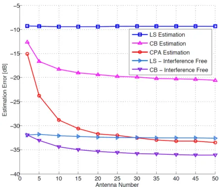
Figure 2.17 - MSE comparison between different estimation techniques and interference free cases, vs. number of base station antennas; source: [56] ... 21

Figure 3.18 - MU-MIMO system model with precoding ... 23

Figure 3.19 - Comb-type pilot structure ... 24

Figure 3.20 - BER plot for different numbers of users and receive antennas ... 27

Figure 3.21 - Block Diagram of MMSE Channel Estimation ... 29

xvi

Figure 3.23 - MSE of transmission to 2 users with MMSE estimator, for different numbers

of pilots... 31

Figure 3.24 - BER plot of transmission to 8 users with MMSE estimator, for different numbers of pilots ... 31

Figure 3.25 - MSE of transmission to 8 users with MMSE estimator, for different numbers of pilots... 32

Figure 3.26 - BER plot of massive MIMO scheme with 64 base station antennas using MMSE estimator, for 𝑁𝑃 = 71 and 𝑁𝑃 = 101 ... 33

Figure 3.27 - MSE plot of massive MIMO scheme with 64 base station antennas using MMSE estimator, for 𝑁𝑃 = 71 and 𝑁𝑃 = 101 ... 33

Figure 3.28 - BER plot of transmission to 2 users with channel estimation using Zadoff-Chu training sequences, for different numbers of pilots ... 36

Figure 3.29 - MSE of transmission to 2 users with channel estimation using Zadoff-Chu training sequences, for different numbers of pilots ... 36

Figure 3.30 - BER comparison between MMSE estimator and ZC method, for 𝑁𝑃 = 7 and 𝑁𝑃 = 31 ... 37

Figure 3.31 - MSE comparison between MMSE estimator and ZC method, for 𝑁𝑃 = 7 and 𝑁𝑃 = 31 ... 37

Figure 3.32 - BER comparison between MMSE estimator and ZC method, for 𝑁𝑃 = 17 and 𝑁𝑃 = 31 ... 38

Figure 3.33 - MSE comparison between MMSE estimator and ZC method, for 𝑁𝑃 = 17 and 𝑁𝑃 = 31 ... 38

Figure 3.34 - MSE of transmission with channel estimation using Zadoff-Chu training sequences, for ranging values of 𝑁𝑢 and 𝑁𝑅 ... 39

Figure 4.35 - Uplink MU-MIMO system model with single-antenna users... 41

Figure 4.36 - Uplink MU-MIMO system model with pilot contamination ... 42

Figure 4.37 - DFE structure ... 43

Figure 4.38 - IB-DFE receiver structure ... 44

Figure 4.39 - IB-DFE performance with perfect CSI knowledge ... 45

Figure 4.40 - BER performance of iterative channel estimation, for 𝑁𝑢 = 𝑁𝑅 = 4, in function of number of iterations and pilots used ... 46

Figure 4.41 - MSE performance of iterative channel estimation, for 𝑁𝑢 = 𝑁𝑅 = 4, in function of number of iterations and pilots used ... 47

xvii

Figure 4.43 - MSE performance of iterative channel estimation, for 𝑁𝑢 = 𝑁𝑅 = 16, in function of number of iterations and pilots used ... 48

Figure 4.44 - BER performance of FSCAPI-based channel estimation, for 𝑁𝑢 = 𝑁𝑅 = 4 and 𝑁𝑢 = 𝑁𝑅 = 16 based on the number of pilots used ... 51 Figure 4.45 - MSE performance of FSCAPI-based channel estimation, for 𝑁𝑢 = 𝑁𝑅 = 4 and 𝑁𝑢 = 𝑁𝑅 = 16 based on the number of pilots used ... 51 Figure 4.46 - BER performance of WPEACH estimator (𝐿 = 8), for 𝑁𝑢 = 𝑁𝑅 = 4 and 𝑁𝑢 = 𝑁𝑅 = 16 based on the number of pilots used ... 54

Figure 4.47 - MSE performance of WPEACH estimator (𝐿 = 8), for 𝑁𝑢 = 𝑁𝑅 = 4 and 𝑁𝑢 = 𝑁𝑅 = 16 based on the number of pilots used ... 55

Figure 4.48 - MSE comparison between channel estimation techniques, for 𝑁𝑢 = 𝑁𝑅 = 4 ... 55 Figure 4.49 - MSE comparison between channel estimation techniques, for 𝑁𝑢 = 𝑁𝑅 = 16 ... 56 Figure 4.50 - BER comparison between channel estimation techniques, for 𝑁𝑢 = 10 and 𝑁𝑅 = 100 ... 56

Figure 4.51 - MSE comparison between channel estimation techniques, for 𝑁𝑢 = 10 and 𝑁𝑅 = 100 ... 57

2

1.

Introduction

1.1

Motivation

In recent decades, we have seen a great evolution in the wireless communications industry. This industry has become increasingly involved in people’s lives, both professionally and personally. The fact of being communicable with the rest of the world has become an all-time necessity and the result is an increasingly demand for wireless connectivity, especially in the last few years. Any Internet user demands fast wireless connections to support all needs, while at the work, at home or on-the-go. Additionally, Machine-to-Machine communications are exponentially growing, leading to an even greater demand of wireless throughput.

To meet the demand, the fifth generation (5G) of wireless communications technology is emerging. 5G is the future of cellular networking and brings new technologies such as millimeter wave (mmWave) communications and massive MIMO systems. Massive MIMO will employ a very high number of antennas to achieve huge gains in both spectral and energy efficiencies. The base stations would serve multiple users at the same time-frequency resource, through spatial multiplexing. The concept is based on the law of large numbers that states that as the number of antennas grows large, the channel responses from different antennas to each user are close to be mutually-orthogonal [1], [2].

3

1.2

Objectives and outline

This work introduces a low-complexity channel estimation technique based on Zadoff-Chu training sequences. In addition, different approaches were studied towards pilot contamination mitigation and lower complexities schemes, with resort to iterative channel estimation methods, semi-blind subspace tracking techniques and matrix inversion alternatives.

4

2.

State of the Art

This chapter begins by describing some basic, but fundamental, features of simple wireless communications systems, in section 2.1. In section 2.2, the motivation, requirements and forthcoming technologies are also presented, followed by a description of the massive MIMO concept and its main advantages and disadvantages. Section 2.2.3 concludes this chapter by presenting the channel estimation topic in massive MIMO systems, how the undesired effect, called pilot contamination, can arise and how to approach it.

2.1

MIMO

In the decade 1970-1980 numerous studies regarding multiple channel transmission systems were published. Among them, [3]–[5] analyze some critical aspects like diversity, sequence estimation, intersymbol and interchannel interference (ISI and ICI respectively) in wired communications, and their mathematical work were valuable for future studies. In 1987, a study was presented describing the fundamental limits on systems with multiple channels in the same bandwidth and the potential for large capacity in systems with limited bandwidth [6]. In 1999, an article was published [7] concerning the problems of communicating over a flat-fading Rayleigh channel using multiple-antenna arrays. In 2001, the first commercial MIMO system was introduced by Iospan Wireless Inc.

5

Figure 2.1 - Radio Propagation

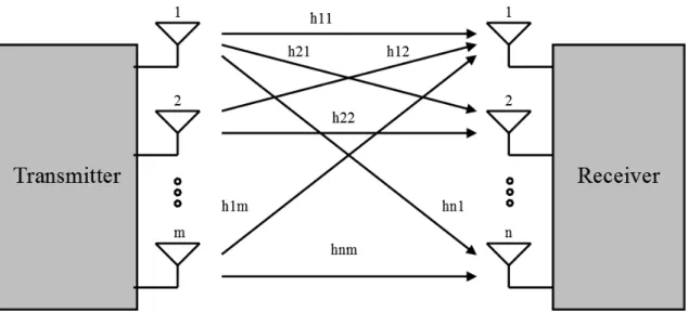
MIMO operates with multiple receive and transmit antennas for signal transmission, as shown in Figure 2.2. Generally, the number of antennas is directly proportional to data rate (multiplexing), quality (diversity) and capacity of the transmission [8], [9]. Besides MIMO, beamforming and space-time coding schemes are another two fundamental technologies that arise in a multiple antennas wireless communication system.

Figure 2.2 - MIMO system model with m transmit antennas and n receive antennas

2.1.1

Diversity and Multiplexing

6

rate of the communication. Adding more antennas at receiver, it is possible to combine every received version of the signal and collectively improve these defects. Diversity can also be applied at the transmitter (called transmit diversity) when multiple antennas send the same signal. The same principle applies, where the probability of the signal reaching the receiver in good conditions is higher than with lesser antennas.

Instead of using multiple antennas to transmit the same signal, each antenna could be used to send different information, in parallel. This technique is called spatial multiplexing and increases the overall capacity of the system.

2.1.2

Beamforming

7

Figure 2.3 – (a) Systems with omnidirectional antennas transmission (b) System with beamforming technique

2.1.3

Channel Estimation

The wireless channel is highly complex and can be frequency- and time-selective due to fading. These phenomena include reflection, diffraction, scattering of the signal and Doppler Shift which represents the change of the frequency from the emitted to the observed wave when the distance between the receiver and the source changes. Therefore, in wireless channels, channel estimation is a vital technique mainly used in mobile wireless network systems. The receiver needs to know exactly the channel state information (CSI) to perform the equalization of the signal and to determine it can be a complex task.

Most of channel estimation techniques use training sequences on transmission. Training sequences are a set of symbols, denominated pilot symbols, known by the receiver that are coupled to the data sequence to be transmitted in order to perform the channel estimation for the next data symbols in which the channel is assumed unchanged, also called coherence time interval. Figure 2.4 depicts a typical time slot structure in systems with channel estimation based on training sequences.

Figure 2.4 - Slot structure in systems with pilot-based channel estimation

8

require training sequences, and for that reason they are denominated as blind-estimation techniques.

2.1.4

Multi-user MIMO

MIMO technology was a big step towards the development of new communication systems. One of them is the multi-user MIMO (MU-MIMO). In a MU-MIMO scheme, the base station communicates with multiple users simultaneously (Figure 2.5).

Figure 2.5 - MU-MIMO system model with 2 users

MU-MIMO schemes offer several advantages over SU-MIMO communications, which are:

 A gain in channel capacity, proportional to the minimum value between the number of BS antennas and the number of antennas at mobile stations, through multi-user multiplexing schemes [11];

 System performance is improved due to the fact that multiple users can communicate over the same spectrum;

 Spatial multiplexing gain at the BS even to single antenna receivers, allowing the arrangement of cheap and small terminals, keeping the more complicated logistics and higher performance costs in the infrastructures side;

 Communications are less affected by channel rank loss, line-of-sight propagation or antenna correlation. Although the aforementioned aspect is increased for each user’s diversity, it can be avoided if multi-user diversity is extracted by the scheduler instead [12].

9

station can manage transmissions from all of its antennas, the receivers are incapable to do so, since users are normally incapable to coordinate their channel information among them. Therefore, the base station must know the CSI perfectly in comparison with regular MIMO schemes, as precoding benefits from a precise CSI estimation. CCI can be canceled by using space-division multiple access (SDMA) schemes. One initial strategy was dirty paper coding (DPC) technique [13], that proves that the sum capacity in a multi-user downlink, or broadcast, channel is equal to the maximum aggregation of all users’ data rates and full multiplexing gain can be achieved. However, DPC is impracticable in real world systems because the high computational complexity involved in coding and decoding schemes [14].

Under the assumption that the base station has an array of transmitting antennas but all users are single-antenna terminals, two low-complexity precoding schemes can be employed to eliminate CCI: Zero-Forcing (ZF) and MMSE. In this case, the receiver considers as interference all external signals and cancels them via precoding. For multiple receiving antennas, block diagonalization (BD) can be used to avoid the usage of DPC method. BD technique will be discussed in Chapter 3.

Precoding schemes such as ZF, MMSE and BD are some alternatives to DPC [15]–[18]. The basis of the abovementioned schemes relies on the surplus of degrees of freedom provided by the excess antennas at the BS, relatively to the users’, to eliminate CCI.

Coordinated beamforming can be also employed to cancel CCI [19], [20]. When there are more users than transmit antennas at the base station, SDMA schemes can achieve full multiplexing gains with transmit beamforming. In larger systems, when the number of users greatly exceeds the number of transmit antennas, low-complexity schemes such as zero-forcing beamforming (ZFBF) [21], [22] or zero-forcing dirty-paper coding (ZF-DPC) [23] were proposed to achieve the optimal growth rate of the sum-capacity function [24].

2.2

Going from MIMO to Massive MIMO

10

2.2.1

Motivation/Requirements

To keep up with this demand, new requirements for mobile traffic need to be achieved, such as [25]:

 Traffic volume – Between the first quarter of 2015 and the first quarter of 2016, data traffic grew 60%. The high volume of traffic data is driven by the increased smartphones subscriptions and high demand for video contents. Total mobile data traffic is expected to rise at a compound annual growth rate (CAGR) of around 45%, resulting in a ten-fold increase in total traffic for all devices by 2021, reaching 52 ExaBytes per month [26] (Figure 2.6).

Figure 2.6 - Global Mobile Traffic (monthly ExaBytes); source: [26]

 Indoor or hotspot traffic – Currently, mobile traffic is mostly common indoor with 60% voice and 70% data traffic. It is anticipated in the future to approach around 90%. Picocells or femtocells are good candidates to achieve higher capacity depending on the environment, quality and type of communication service, although the deployment of femtocells is proved to be more efficient in indoor environments than picocells as it achieves the highest in-building capacity [27].

11

Figure 2.7 - Mobile Subscriptions by Technology (billion); source: [26]

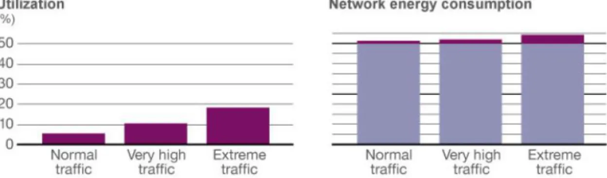
 Energy consumption – An essential requirement is to deliver high network energy performance in order to follow up the required traffic volume forecasted, to reduce the total cost of ownership (TCO) and to ease the access of network connectivity in remote areas. In a classic long term evolution (LTE) network, more than 90% of energy consumption of total traffic usage is for the network to be detectable and accessible, regardless the traffic load volume, as shown in Figure 2.8.

Figure 2.8 - Utilization and corresponding network energy consumption for different traffic loads; source: [28]

12

2.2.2

Innovations

In order to achieve the previous requirements, wireless network technologies have to be improved and for that purpose some revolutionary features are under development such as Millimeter Wave (mmWave) communications and Massive MIMO systems. The main objective of MmWave communications is to reach an unexplored range of higher frequencies of the spectrum and Massive MIMO is to expand the antenna arrays to a whole new level.

2.2.2.1

Millimeter Waves Communications

Radio frequencies (RF) are used on almost all commercial communications in a narrow band between 300 MHz and 3 GHz. Therefore, its spectrum is increasingly scarce and getting access to it becomes a harder task as time goes by. Current efforts are only based on reusing and sharing the spectrum and do not achieve the upcoming requirements [29]. The only way to achieve large amounts of new bandwidth is to use higher frequencies, somewhere between the 3 GHz and 300GHz, where the millimeter wave (mmWave) spectrum is less crowded and much greater bandwidths are available. However, not all spectrum can be used since in some frequency ranges oxygen molecules and water vapor absorb electromagnetic energy (57 GHz – 64 GHz and 164 GHz – 200 GHz, respectively), as shown in Figure 2.9. Excluding these frequencies, mmWave communications could achieve around 100GHz of new bandwidth, 200 times more than the currently allocated spectrum, below 3 GHz [30].

In terms of free space loss, there is no difference by using different frequencies for the same antenna aperture. Furthermore, higher frequency means shorter wavelengths which lead to a higher density of antennas in mobile devices and infrastructures and it also improves non-line-of-sight communications, contrarily to current MIMO systems.

13

Figure 2.10 depicts a data rate comparison in terms of mean and 5% outage rates. Results are given in terms of gain with regards to the MIMO baseline. It is clear that millimeter wave systems could lead to unmatched data rates and revolutionary user experience as a potentially innovative technology for 5G.

Figure 2.10 - Data rate comparison between microwave systems using 50 MHz of bandwidth (SISO and SU-MIMO) and a single user mmWave system with 500 MHz of bandwidth; source: [31]

On the other hand, the wave’s frequency is inversely proportional to penetration capability. The analysis of [32] and [33] concludes that millimeter wave signals are highly attenuated by commonly solid materials such as concrete or brick walls, about 10 times more at 40 GHz than radio wave frequencies below 3 GHz. A solution to this problem involves the placement of mmWave femtocells inside buildings for indoor coverage.

Another two problems are the difficult propagation of mmWave transmissions through foliage and the signal scattering in raindrops. For the first case, an empirical relationship has been developed [34], that predicts the foliage loss in a range of frequencies between 200-95000 MHz in foliage depths lesser than 400 meters. As an example, at 40 GHz, a signal penetrating a large tree, around 10 meters, is about 19 dB. For the second case, raindrops have approximately the same size as the radio wavelengths, causing the scattering of the radio signal. For example, at 50 GHz, with a rain rate of 25mm/h, there is a 10db/km attenuation of the signal, as shown [34].

14

2.2.2.2

Massive MIMO

The primary idea behind massive MIMO systems is to massively scale up MU-MIMO systems, by deploying a huge number of antennas in transmitters/receivers, in the order of hundreds or more. In massive MIMO systems, the number of antennas in base stations excessively surpass the number of active users. Moreover, the base station serves all active users, simultaneously, in the same time-frequency resource.

In communications systems with few antennas, signal strength can be momentarily very low due to fading. This happens when scattered signals reach the receiver and the combined waves interfere destructively with each other and the only solution is to wait until the channel has changed enough so the data can be properly received. This delay in reception is called latency. However, as the law of large numbers predicts, if the number of scattered signals is largely increased and the number of antennas is increased as well, it will be more likely that the received signal will be closer to the expected, so fading no longer limits latency. Another result of the large number of antennas is shown in [1] where using a number of base station antennas that greatly exceeds the number of active users linear processing is nearly optimal (with single-antenna users). Additionally, by using maximum-ratio combining (MRC) or maximum-ratio transmission (MRT) in uplink or downlink, respectively, the effects of uncorrelated noise and intracell interference tend to disappear because, as the law of large numbers implies, the channel matrix for a desired user tends to be more orthogonal to an interfering user channel matrix, rendering simple spatial multiplexing procedures with optimal results. Massive MIMO also provides a large excess of degrees of freedom, which can be exploited to provide extremely cheap and power efficient RF amplifiers [36], [37].

15

Figure 2.11 - Spectral efficiency vs. Energy efficiency in SISO, MISO and Massive MIMO systems with different processing methods; source: [39]

In practice, deploying very large arrays is a spatially dimensional problem. Since antennas have to be distributed half-wavelength apart, 100 antennas can occupy almost one meter of space. Though, mmWave technology eases this problem since the resort to higher frequencies allows much smaller dimension antennas designs [40]. Furthermore, architectural issues of using larger arrays were already proposed in [41]–[45].

16

Figure 2.12 - Downlink sum-rate capacity with DPC, for 16 users in different user inter-location scenarios; source: [46]

2.2.3

Channel Estimation in Massive MIMO

17

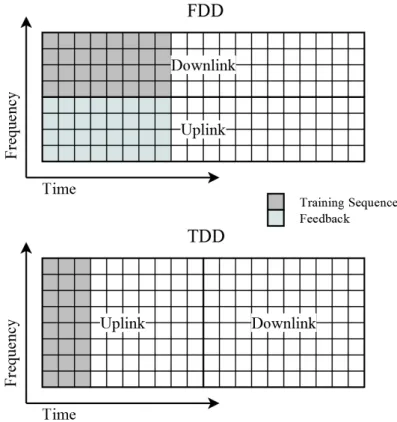
Figure 2.13 –Time slot with channel estimation for FDD and TDD systems

Despite the use of FDD in the current LTE standard, incorporating a FDD strategy is more difficult in massive MIMO systems due to orthogonality issues between antennas and large number of required channel estimations. Downlink pilots must be mutually orthogonal for optimal estimations. To accomplished that, time-frequency resources are spent proportionally to the number of antennas at the base station, which requires hundreds of times more resources in massive MIMO systems than in conventional MIMO. The number of orthogonal training sequences must be smaller than the number of pilots on the training sequences.

Another problem lies in the number of estimations to be done by the terminals in the minimum amount of time. The number of channel responses that have to be estimated by each user is proportional to the number of base station antennas. Therefore, the terminals would have to spent hundreds of times more resources to feedback the base station with the channel responses estimates, which is a critical drawback for mobile devices, and the need to feedback adds latency to transmission. Moreover, the estimated CSI can also be deteriorated by quantization errors due to the limited channel feedback and outdated due to the delay between the moment the estimation was performed and its implementation at base station. In the work of [48] the case of non-ideal CSI is analyzed at base stations and specifically the trade-off between the advantage of large number of antennas and the cost of estimating large channel vectors, in FDD systems.

18

MIMO systems, since the required pilot resources are independent of the number of base station antennas, or FDD schemes that require a considerably reduced CSI accuracy [49].

2.2.3.1

Pilot Contamination

Since massive MIMO is supposed to be a practical cellular network, it is distributed along multiple cells, as a multicell system. For channel estimation, every terminal has a correspondent training sequence to eliminate intra-cell interference. Additionally, channel estimation must be performed during each coherence interval, and for that reason, the number of mutually orthogonal training sequences must be smaller than the number of elements in each coherence interval. So, depending on the number of coherent time-frequency elements, the training sequences must be reused in other cells. Due to this limitation, pilot contamination may happen. A signal suffers from pilot contamination, when a receiver gets the same pilot sequence from different sources of different cells resulting in an incorrect channel estimate (Figure 2.14). Therefore, pilot contamination limits the performance of non-cooperative MU-MIMO systems [1].

Figure 2.14 - Pilot contamination example when both users transmit mutually non-orthogonal training sequences

As the base station estimates inaccurately the desired channel responses, the precoding performed on the transmitted signal is also incorrect. The erroneous precoding decreases significantly the signal-to-interference-plus-noise ratio (SINR) of the whole transmission. Since the base station performs beamforming, in a MRT precoding scheme, the signal power is misplaced due to the estimated channel values, i.e., the desired user receives a less powered signal, and the power lost is redirected as interference to the undesired users with the same training sequence.

19

active users. In practice, to allow data transmission with good spectral efficiency as well, the number of terminals has to be significantly smaller than the number of symbols in the coherence interval. Thus, pilot contamination becomes a major problem in a massive MIMO scenario. As concluded in [50], it causes the saturation of SINR as the number of base station antennas tends to infinity. Figure 2.15 shows that as the path-loss gain (ratio between the path-loss coefficients for the channels of desired user and interfering user) increases, the saturation value of SINR also increases.

Figure 2.15 - Variation of SINR and its approximation for different path-loss gains (2 and 2,5) at 10dB interference-free SNR; source: [50]

Numerous methods for pilot contamination mitigation have already been proposed. In [51] a completely-blind method of pilot decontamination for uplink transmission is proposed, although, by exploiting channel reciprocity in TDD schemes, the same strategy can be applied. [52] employs a pilot contamination precoding (PCP) scheme among multiple cells, addressed to terminals with the same pilot sequence.

20

covariance of received training sequence. However, EVD and EEVD techniques are founded on a critical assumption: the number of antennas at base station tends to infinity, and, therefore, performance degradation is expected, by pilot contamination, as the number of antennas is finite. Moreover, eigenvalue decomposition is a nonlinear operation, so, for large matrices, approximation errors and high computational requirements are severe problems to be taken into account. Figure 2.16 presents the MSE between the two abovementioned channel estimation techniques in function of the number of transmit antennas.

Figure 2.16 - MSE performance between EVD and EEVD channel estimation vs. the number of base station antennas, M; source: [54]

21

22

3.

Channel Estimation Techniques

Massive MIMO has shown to be a promising concept in 5G cellular networks. The increased number of antennas at the base station combined with MU-MIMO transmission techniques make massive MIMO more energy-efficient and capable to reach higher spectral efficiency. A major restrictive factor in massive MIMO is the availability of an accurate CSI, since spatial multiplexing can only be achieved if the channel responses are precisely known. For that reason, channel estimation is a main subject to be discussed in wireless communications systems, primarily when the future of the industry probably will involve a large scaling of antenna arrays.

This chapter begins by describing the adopted MU-MIMO downlink system model, followed by an explanation of the BD method, used to cancel CCI, and two low-complexity channel estimators commonly used in nowadays communication systems: LS and MMSE channel estimator. Additionally, it is introduced a channel estimation technique using Zadoff-Chu sequences as pilot signals. These sequences possess ideal periodic autocorrelation properties, which makes them ideal to be considered training sequences. To conclude the chapter, are presented the simulation results that allow a comparison purposes between the different channel estimation techniques. Simulations results will demonstrate how accurate the introduced channel estimation is, in function of the number of users and the number of pilots applied in estimation. BER and MSE are used as performance measurement and comparison purposes. Results are based on Monte Carlo experiments with 15 000 simulations and QPSK modulation. Both BER and MSE results are expressed in function of 𝐸𝑏

𝑁0, where 𝐸𝑏 is the transmitted bit energy and where 𝑁0 is the noise power spectral density.

3.1

System Model

The system model adopted is a downlink orthogonal frequency-division multiple access (OFDMA) transmission over a multi-user precoding MIMO system with 𝑁_𝑢 users, 𝑁_𝑅 receiving antennas at each mobile station and 𝑁_𝑇 = 𝑁_𝑢𝑁_𝑅 transmitting antennas at the base station, resulting in a 𝑁_𝑇×𝑁_𝑅 MIMO configuration to each user 𝑢, with 𝑁 subcarriers, through a channel 𝑯𝑢𝐷𝐿 (𝑯𝑢𝐷𝐿𝜖ℂ𝑁𝑅×𝑁𝑇), depicted in Figure 3.18.

23

Figure 3.18 - MU-MIMO system model with precoding

The received signal for every user is given by

[ 𝒚1 𝒚2 ⋮ 𝒚𝑁𝑢

] = [ 𝑯1𝐷𝐿

𝑯2𝐷𝐿 ⋮ 𝑯𝑁𝑢𝐷𝐿]

𝑿 + [ 𝒛1 𝒛2 ⋮ 𝒛𝑁𝑢

] , (1)

or simply by

𝒀𝐵𝐶 = 𝑯𝐷𝐿𝑿 + 𝒁 , (2)

where 𝒚_𝑢 (𝒚_𝑢𝜖ℂ𝑁𝑅_{) is the received signal at the} 𝑢_{-th user (}𝑢 = 1,2, … , 𝑁_𝑢), 𝑿 ₍𝑿𝜖ℂ𝑁𝑇_{) is the} transmitted signal by the BS, and 𝒛_𝑢 (𝒛_𝑢𝜖ℂ𝑁𝑅_{) is the array relative to additive white gaussian} noise (AWGN) with zero mean and variance 𝜎_𝑧2=𝑁0

2.

The channel matrix 𝑯_𝑢𝐷𝐿 contains all SISO channel impulse responses from each BS transmitting antenna to each receiving antenna of a single user. The elements of 𝑯_𝑢𝐷𝐿 are samples of independent and identically distributed (i.i.d.) complex Gaussian process, given by

𝑯𝑢𝐷𝐿= [

ℎ1,1 … ℎ1,𝑁𝑇

⋮ ⋱ ⋮

ℎ𝑁𝑅,1 … ℎ𝑁𝑅,𝑁𝑇

] . (3)

The signal received by a single user is given by

𝒚𝑢 = [ 𝑦1 𝑦2 ⋮ 𝑦𝑁𝑅

] = [ℎ1,1⋮ … ℎ⋱ 1,𝑁⋮ 𝑇 ℎ𝑁𝑅,1 … ℎ𝑁𝑅,𝑁𝑇

] [ 𝑥1 𝑥2 ⋮ 𝑥𝑁𝑇

] + 𝒛𝑢 , (4)

and, therefore, each antenna receives the signal

24

3.1.1

Channel Model

The channel considered is a frequency-nonselective or frequency flat fading channel given by [57]:

ℎ𝑛𝑟,𝑛𝑡(𝑡) = 𝛼(𝑡)𝑒𝑗𝜃(𝑡) , ∀𝑛𝑟, 𝑛𝑡 , (5)

where 𝛼(𝑡) denotes the envelope and 𝜃(𝑡) represents the phase of the equivalent channel response. This means the coherence bandwidth, 𝐵_𝑐𝑜ℎ, is larger than the signal bandwidth, 𝐵_𝑆 i.e.,

𝐵𝑆≪ 𝐵𝑐𝑜ℎ . (6)

Hence, all frequencies of the transmitted signal experience equal gain and linear phases during the duration of a OFDM symbol. Then, the channel has a time-varying multiplicative effect on the transmitted signal.

3.1.2

Pilot Structure

There are three different types of pilots’ structures that can be adopted: block type, comb type, and lattice type [58]. In the model adopted here, the pilots are arranged in a comb type format, as shown in Figure 3.19. Comb type pilot arrangement are regularly used for fast-fading channel characteristics, but not for frequency-selective channels [59], [60].

Figure 3.19 - Comb-type pilot structure

25

frequency-flat over each symbol, the estimates are used in equalization for the next 𝑁_{𝑑𝑎𝑡𝑎} subcarriers (𝑁_{𝑑𝑎𝑡𝑎} = 𝑁 − 𝑁_𝑃).

3.2

Block Diagonalization

In MU-MIMO systems with single-antenna users, precoding methods based on channel inversion are used to eliminate interference between antennas. However, in MU-MIMO systems, precoding eliminates the interference across different users but not between different antennas. So the sum capacity of the system can be increased with diversity. In these scenarios, BD is a common technique used in linear precoding schemes. This method is a generalization of channel inversion and resorts to a non-linear process called singular value decomposition (SVD). After performing BD, any signal detection method can be applied to eliminate inter-antenna interference.

In BD, each user is associated to a precoding matrix. The precoding matrix is generated in a way that the base station transmits the signal to the user through the null space of all other interfering users. Overall, the aggregated MU-MIMO channel matrix of all users is decomposed into multiple, parallel, independent SU-MIMO sub-channels corresponding to each user. However, the non-linearity process forces channel estimation to be more accurate than in a standard MIMO system.

The precoded signal for the 𝑢-th user can be written as:

𝒙𝑢= 𝑾𝑢𝒙̃𝑢 , 𝑢 = 1, 2, … , 𝑁𝑢 , (7) where 𝒙_𝑢 (𝒙_𝑢𝜖ℂ𝑁𝑇_{) is the coded array of transmitting symbols,} 𝑾_{𝑢 (}𝑾_𝑢𝜖ℂ𝑁𝑇×𝑁𝑅_{) the precoding} matrix and 𝒙̃_𝑢 (𝒙̃_𝑢𝜖ℂ𝑁𝑅_{) is the vector with} 𝑁_{𝑅 parallel data symbols concerning the user} 𝑢_{. The} signal that each user 𝑢 receives can be expressed as:

𝒚𝑢 = 𝑯𝑢𝐷𝐿∑ 𝑾𝑘𝒙̃𝑘 𝑁𝑢

𝑘=1

+ 𝒛𝑢 , 𝑢 = 1, 2, … , 𝑁𝑢 . (8)

The same equation can be rearranged as

𝒚𝑢= 𝑯𝑢𝐷𝐿𝑾𝑢𝒙̃𝑢+ ∑ 𝑯𝑢𝐷𝐿𝑾𝑘𝒙̃𝑘 𝑁𝑢

𝑘=1,𝑘≠𝑢

+ 𝒛𝑢 , 𝑢 = 1, 2, … , 𝑁𝑢 , (9)

where 𝑯_𝑢𝐷𝐿𝑾_𝑘 is an effective channel matrix for the 𝑢-th user receiver and the 𝑘-th user transmit signal (𝑢, 𝑘 = 1,2, … , 𝑁_𝑢). In matrix format, the received signals are represented as:

[ 𝒚1 𝒚2 ⋮ 𝒚𝑁𝑢

] = [

𝑯1𝐷𝐿𝑾1 𝑯1𝐷𝐿𝑾2 … 𝑯1𝐷𝐿𝑾𝑁𝑢 𝑯2𝐷𝐿𝑾1 𝑯2𝐷𝐿𝑾2 … 𝑯2𝐷𝐿𝑾𝑁𝑢

⋮ ⋮ ⋱

𝑯𝑁𝑢𝐷𝐿𝑾1 𝑯𝑁𝑢𝐷𝐿𝑾2 𝑯𝑁𝑢𝐷𝐿𝑾𝑁𝑢] [

𝒙̃1 𝒙̃2 ⋮ 𝒙̃𝑁𝑢

] + [ 𝒛1 𝒛2 ⋮ 𝒛𝑁𝑢

26

when 𝑯_𝑢𝐷𝐿𝑾_𝑘 ≠ 0_{𝑁𝑅×𝑁𝑅}, ∀ 𝑢 ≠ 𝑘 there is CCI, where 0_{𝑁𝑅×𝑁𝑅} is a zero matrix. From (10) it can be seen that CCI-free transmission is guaranteed as long as the effective channel matrix is block-diagonalized, to ensure that

𝑯𝑢𝐷𝐿𝑾𝑘= 0𝑁𝑅×𝑁𝑅, ∀ 𝑢 ≠ 𝑘 . (11) Let denote 𝑯̃_𝑢𝐷𝐿 (𝑯̃_𝑢𝐷𝐿ℂ𝑁𝑅(𝑁𝑢−1)×𝑁𝑇_{) as the congregate interfering channel matrix that} contains the channel responses of all users except the 𝑢-th user

𝑯̃𝑢𝐷𝐿= [(𝐻1𝐷𝐿)𝐻 … (𝐻𝑢−1𝐷𝐿)𝐻 (𝐻𝑢+1𝐷𝐿)𝐻 … (𝐻𝑘𝐷𝐿)𝐻] 𝐻

, (12)

where (•)𝐻 denotes the complex-conjugate transpose operation, or Hermitian transpose. Thus, since 𝑁_𝑇 = 𝑁_𝑅𝑁_𝑢, (11) is equivalent to

𝑯̃𝑢𝐷𝐿𝑾𝑢= 0(𝑁𝑇−𝑁𝑅)×𝑁𝑅 , 𝑢 = 1, 2, … , 𝑁𝑢 . (13) Therefore, results a CCI-free transmission:

𝒚𝑢= 𝑯𝑢𝐷𝐿𝑾𝑢𝒙̃𝑢+ 𝒛𝑢. (14)

which corresponds in matrix format to

[ 𝒚1 𝒚2 ⋮ 𝒚𝑁𝑢

] = [

𝑯1𝐷𝐿𝑾1 0 … 0

0 𝑯2𝐷𝐿𝑾2 … 0

⋮ ⋮ ⋱

0 0 𝑯𝑁𝑢𝐷𝐿𝑾𝑁𝑢] [

𝒙̃1 𝒙̃2 ⋮ 𝒙̃𝑁𝑢

] + [ 𝒛1 𝒛2 ⋮ 𝒛𝑁𝑢

] . (15)

The interference can be cancelled using the diagonalization process called SVD [61], [62]. To obtain the precoding matrix 𝑾_𝑢 which satisfies the condition of (13). It is possible to separate 𝑯̃𝑢𝐷𝐿 into a product of three matrices.

𝑯̃𝑢𝐷𝐿= 𝑼̃𝑢𝚲̃𝑢𝑽̃𝑢𝐻 , (16)

where 𝑼̃_𝑢 (𝑼̃_𝑢 𝜖ℂ𝑁𝑅(𝑁𝑢−1)×𝑁𝑅(𝑁𝑢−1)_{) and 𝑽̃𝑢 (𝑽̃𝑢 𝜖ℂ}𝑁𝑇×𝑁𝑇_{) are orthogonal matrices and} 𝚲̃𝑢 (𝚲̃𝑢𝜖ℂ𝑁𝑅(𝑁𝑢−1)×𝑁𝑇) is a diagonal matrix containing the square roots of eigenvalues from 𝑼̃𝑢 or 𝑽̃_𝑢. Since 𝚲̃_𝑢 will not be a square matrix, there will be empty columns. In that case, 𝑽̃_𝑢 can be represented as

27 𝑯̃𝑢𝐷𝐿𝑽̃𝑢𝑍 = 𝑼̃𝑢[𝚲̃𝑢𝑁𝑍 0] [(𝑽̃𝑢

𝑁𝑍₎𝐻 (𝑽̃𝑢𝑍)𝐻

] 𝑽̃𝑢𝑍

= 𝑼̃𝑢𝚲̃𝑢𝑁𝑍(𝑽̃𝑢𝑁𝑍)𝐻𝑽̃𝑢𝑍 = 𝑼̃𝑢𝚲̃𝑢𝑁𝑍0

= 0 ,

(18)

which means that when the signal is transmitted in the direction of 𝑽̃_𝑢𝑍, every interfering user will not receive any signal. Therefore, 𝑽̃_𝑢𝑍 will be the precoding matrix for user 𝑢, given by

𝑾𝑢= 𝑽̃𝑢𝑍 . (19)

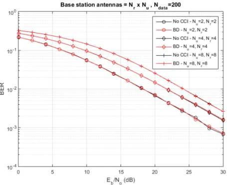
Figure 3.20 shows the effectiveness of BD method in eliminating CCI. When compared to a CCI-absent transmission scheme in the same conditions.

Figure 3.20 - BER plot for different numbers of users and receive antennas

28

3.3

One Dimension Channel Estimators

LS channel estimator and MMSE channel estimator are two basic, pilot-based channel estimation techniques. These estimators are categorized as one dimension (1D) estimators, this means that the channel estimation is done by resorting to training sequences, of length 𝑁_𝑃, in one dimension, either in frequency or time domain. Due to their simplicity they are widely used for pilot-based channel estimation [54], [58-60].

3.3.1

Least-Squares Channel Estimation

The LS channel estimator minimizes the squared error quantity between the received signal and the estimated one and may be described as

𝒉̂𝐿𝑆_{= arg}

𝒉̃𝐿𝑆min‖𝒚 − 𝒉̃𝐿𝑆𝑺‖ 2

, (20)

where 𝑺 (𝑺𝜖ℂ𝑁𝑇×𝑁𝑃_{) is the matrix containing the transmitted training sequences} 𝒔_𝑛𝑡 (𝑛𝑡 = 1,2, … , 𝑁𝑇) of all transmit antennas such as:

𝑺 = [ 𝒔1 𝒔2 ⋮ 𝒔𝑁𝑇

] . (21)

The channel estimates of the channel impulse responses between all transmit antennas and the 𝑛-th receiving antenna are given by

𝒉̂𝑛𝐿𝑆 = 𝒚𝑛𝑺𝐻[𝑺𝑺𝐻]−1 , (22)

or, generically, for non-white Gaussian noise by

𝒉̂𝑛𝐿𝑆 = 𝒚𝑛𝑹𝑧𝑧−1𝑺𝐻[𝑺𝑹𝑧𝑧−1𝑺𝐻]−1 , (23) where (•)−1 denotes the inverse operation and 𝑹_𝑧𝑧 is the auto-correlation matrix of the noise given by:

𝑹𝑧𝑧= 𝜎𝑧2𝑰𝑁𝑅×𝑁𝑅 , (24)

where 𝑰_{𝑁𝑅×𝑁𝑅} is the identity matrix.

The MSE of the LS channel estimate is equal to: 𝑀𝑆𝐸𝐿𝑆 =𝜎𝑧

2

𝜎𝑥2 . (25)

29

when the channel is in deep fading. However, since this technique does not consider channel statistical parameters, it is extensively used for channel estimation.

3.3.2

Minimum Mean-Square Error Channel Estimation

MMSE channel estimation is a more accurate version of the LS channel estimation. Let us consider the block diagram shown in Figure 3.21, where 𝑴 is the weight matrix and 𝒉̂𝑀𝑀𝑆𝐸 corresponds to the MMSE estimate.

Figure 3.21 - Block Diagram of MMSE Channel Estimation

The MMSE channel estimator minimizes the MSE between the true channel, 𝑯, and the MMSE estimated channel, 𝒉̂𝑀𝑀𝑆𝐸, by finding a good linear estimate in terms of 𝑴 and the value of LS estimate, 𝒉̂𝐿𝑆:

𝒉̂𝑀𝑀𝑆𝐸_{= arg}

𝒉̃𝑀𝑀𝑆𝐸min‖𝑯 − 𝒉̃𝑀𝑀𝑆𝐸‖ 2

, (26)

with

𝒉̂𝑀𝑀𝑆𝐸_{= 𝒉̂}𝐿𝑆_{𝑴 . (27)}

According to the principle of orthogonality, the estimation error vector 𝜀 = 𝑯 − 𝒉̂𝑀𝑀𝑆𝐸 is orthogonal to 𝒉̂𝐿𝑆, resulting in

𝑹_𝑯𝒉̂𝐿𝑆− 𝑴𝑹_𝒉̂𝐿𝑆_𝒉̂𝐿𝑆= 0 , (28) where 𝑹_𝑯𝒉̂𝐿𝑆 represents the cross-correlation matrix between 𝑯 and 𝒉̂𝐿𝑆, and 𝑹_𝒉̂𝐿𝑆_𝒉̂𝐿𝑆 the auto-correlation matrix of 𝒉̂𝐿𝑆 given by

𝑹_𝒉̂𝐿𝑆_𝒉̂𝐿𝑆= 𝑹_𝑯𝑯+𝜎𝑧 2 𝜎𝑥2𝑰 .

(29) Solving (28) in function of 𝑴 results:

30 𝒉̂𝑀𝑀𝑆𝐸_{= 𝒉̂}𝐿𝑆_𝑹

𝑯𝒉̂𝐿𝑆(𝑹_𝑯𝑯+𝜎𝑧 2 𝜎𝑥2𝑰)

−1

. (31)

Assuming that every channel response energy is normalized, such as:

𝐸 {|ℎ𝑛𝑟,𝑛𝑡|2} = 𝜎ℎ2 , ∀𝑛𝑟, 𝑛𝑡 , (32) the estimate solution of the Equation (31) for the 𝑛-th receiving antenna can be simplified to:

𝒉̂𝑛𝑀𝑀𝑆𝐸 = 𝒙𝑛𝑺𝐻(𝑺𝑺𝐻+𝜎𝑧 2 𝜎ℎ2𝑰)

−1

. (33)

Generally, for non-white Gaussian noise we have

𝒉̂𝑛𝑀𝑀𝑆𝐸= 𝒙𝑛𝑹𝑧𝑧−1𝑺𝐻(𝑺𝑹𝑧𝑧−1𝑺𝐻+𝜎𝑧 2 𝜎ℎ2𝑰)

−1

. (34)

Since MMSE estimation relies on minimizing the MSE, it has a better performance than LS channel estimation. The downside lies on the fact that it depends on the channel statistics. Hence, this method has a higher complexity than the LS estimator. To reduce the complexity of MMSE channel estimator, a technique called modified MMSE is suggested in [63].

In this work, the MSE of the estimated channel is defined as

𝑀𝑆𝐸 =‖𝑯𝑢

𝐷𝐿_{− 𝑯̂}

𝒖

𝑀𝑀𝑆𝐸_‖

𝐹 𝑁𝑇𝑁𝑅

(35) where ‖•‖_𝐹 denotes the Frobenius norm of a matrix.

Figure 3.22 and Figure 3.23 show the BER and MSE results, to compare the accuracy of the MMSE estimator for a different numbers of pilots in a scheme with 2 users and 2 receive antennas per each one.

31

Figure 3.23 - MSE of transmission to 2 users with MMSE estimator, for different numbers of pilots

It is clear that for 𝑁_𝑃 = 7, estimation performance is degraded, but for the other values of 𝑁_𝑃 the estimation is accurate. Obviously, as the number of pilots increase, the channel estimation is more precise. The following plots, Figure 3.24 and Figure 3.25, consider an 8 users scheme for the same comparison purposes as before.

32

Figure 3.25 - MSE of transmission to 8 users with MMSE estimator, for different numbers of pilots

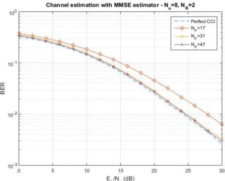
When the number of pilots is close to the number of base station antennas (𝑁_𝑇 = 4, 𝑁_𝑃= 7 for the first case, and 𝑁_𝑇 = 16, 𝑁_𝑃= 17 for the second one), it is visible a degradation in the performance of the estimators. Apart from that, for the rest of the set of training sequence lengths the BER plot shows an approximated performance to the exact CSI.

33

Figure 3.26 - BER plot of massive MIMO scheme with 64 base station antennas using MMSE estimator, for 𝑁_𝑃= 71 and 𝑁_𝑃= 101

Figure 3.27 - MSE plot of massive MIMO scheme with 64 base station antennas using MMSE estimator, for 𝑁_𝑃= 71 and 𝑁_𝑃= 101

34

3.4

Channel Estimation with Zadoff-Chu training sequences

Zadoff-Chu (ZC) sequences are complex-valued mathematical sequences in which cyclically shifted versions of the same sequence are orthogonal to each other, that is, they have zero correlation. A non-shifted sequence is known as “root sequence” and is defined as:

𝑥𝑈(𝑛) = 𝑒−𝑗𝜋𝑈𝑛(𝑛 + 1)_𝑁

𝑍𝐶 , 0 ≤ 𝑛 ≤ 𝑁𝑍𝐶 , (36)

where 𝑈 is the root index that determines a specific sequence, 𝑛 is the time index and 𝑁_𝑍𝐶 is the length of the sequence. If 𝑁_𝑍𝐶 is a prime number, each root index (𝑈 = 1,2, … , 𝑁_𝑍𝐶− 1) generates different Zadoff-Chu sequences.

Zadoff-Chu sequences belong to the class of perfect polyphase sequences [66], also called Constant Amplitude Zero Autocorrelation (CAZAC) sequences. A CAZAC sequence is a periodic signal with modulus one and discrete cyclic autocorrelation equal to zero, i.e., each circularly shifted version of the same sequence is mutually orthogonal. Hence, the discrete Fourier transform (DFT) of any Zadoff-Chu sequence has constant amplitude. Furthermore, the cross-correlation between two prime-length Zadoff-Chu sequences of different root indices coprimes to 𝑁_𝑍𝐶 is constant and equal to √𝑁_𝑍𝐶.

Zadoff-Chu sequences are used in several channels of LTE standard, more specifically in primary synchronization signal (PSS), reference signal (RF) both uplink and downlink, physical uplink control channel (PUCCH), physical uplink traffic channel (PUSCH) and physical random access channel (PRACH).

Since all cyclically shifted versions of a Zadoff-Chu sequence are orthogonal to each other, they can be used as training sequences for channel estimation in transmissions with multiple antennas, simultaneously.

Let us assume 𝑺 as the matrix containing the transmitted training sequences, in (21). Each training sequence 𝒔_𝑛𝑡(𝑛𝑡 = 1,2, … , 𝑁_𝑇)is a circularly shifted version of a Zadoff-Chu sequence with the same root index, of length 𝑁_𝑍𝐶, so,

⟨𝒔𝑎, 𝒔𝑏⟩ = 0 , 𝑎 ≠ 𝑏 , (37)

where ⟨•, •⟩ refers to the Hermitian inner product operation.

Subsequently, the constraint 𝑁_𝑍𝐶> 𝑁_𝑇 is imposed so every sequence is pairwise orthogonal and, therefore, each channel response is distinguished. This is a major drawback in massive MIMO systems, where 𝑁_𝑇 is intended to be large.

In reception, the 𝑛𝑟-th receive antenna (𝑛𝑟 = 1,2, … , 𝑁_𝑅) obtains the following signal: 𝒚𝑛𝑟= 𝒔1ℎ𝑛𝑟,1+ 𝒔2ℎ𝑛𝑟,2+ ⋯ + 𝒔𝑛𝑟ℎ𝑛𝑟,𝑛𝑡+ ⋯ + 𝒔𝑁𝑇ℎ𝑛𝑟,𝑁𝑇 ,

(𝑛𝑡 = 1,2, … , 𝑛𝑟, … , 𝑁𝑇) .

35

So, ℎ_{𝑛𝑟,𝑛𝑡}(𝑛𝑡 = 𝑛𝑟) is the desired channel while ℎ_{𝑛𝑟,𝑛𝑡}(𝑛𝑡 ≠ 𝑛𝑟) are the interfering channels.

Therefore, using the Hermitian inner product operation in 𝒚_𝑛𝑟 with the appropriate training sequence 𝒔_𝑛𝑟 the unwanted interference parcels will be canceled, resulting

⟨𝒚𝑛𝑟, 𝒔𝑛𝑟⟩ = |𝒔𝑛𝑟|2ℎ̅𝑛𝑟,𝑛𝑟 , (39) where |•| refers to the norm function and •̅ denotes the complex conjugate.

Since the square of a vector’s norm is equal to the length of the vector, the expression can be simplified as:

⟨𝒚𝑛𝑟, 𝒔𝑛𝑟⟩ = 𝑁𝑍𝐶ℎ̅𝑛𝑟,𝑛𝑟 . (40) Thus, to estimate the value of the corresponding channel response, ℎ̂_{𝑛𝑟,𝑛𝑟}, it is just needed to divide by 𝑁_𝑍𝐶 and proceed with complex conjugate operation.

ℎ̂𝑛𝑟,𝑛𝑟 =⟨𝒚𝑛𝑟, 𝒔𝑛𝑟⟩ ̅̅̅̅̅̅̅̅̅̅̅̅ 𝑁𝑍𝐶 .

(41) This estimator does not perform matrix inversions and, therefore, it has much lower complexity than a MMSE estimator, specially in a massive MIMO scenario, where the channel matrix is very large.

36

Figure 3.28 - BER plot of transmission to 2 users with channel estimation using Zadoff-Chu training sequences, for different numbers of pilots

Figure 3.29 - MSE of transmission to 2 users with channel estimation using Zadoff-Chu training sequences, for different numbers of pilots

37

the number of base station antennas, but in the length of the training sequences. Plus, the number of receive antennas equipped at each user enhances the MSE results, as depicted in Figure 3.34.

Figure 3.30 - BER comparison between MMSE estimator and ZC method, for 𝑁_𝑃= 7 and 𝑁_𝑃= 31

38

Figure 3.32 - BER comparison between MMSE estimator and ZC method, for 𝑁_𝑃= 17 and 𝑁_𝑃= 31

39

Figure 3.34 - MSE of transmission with channel estimation using Zadoff-Chu training sequences, for ranging values of 𝑁_𝑢 and 𝑁_𝑅

40

4.

Pilot Contamination

Channel estimation has an important role in massive MIMO transmission, in order to reduce CCI. However, the reuse of training sequences in neighboring cells imposes a limitation on the achievable rate in a massive MIMO system. This limitation arises from the phenomenon called pilot contamination. The number of distinct training sequences should be higher than the number of users that are being served in the system. Moreover, the number of mutually orthogonal training sequences that can be generated is upper bounded by the length of those sequences. Thus, there is a tradeoff between the length of the training sequences and the data transmission payload. The tradeoff worsens as the channel coherence interval becomes smaller. In order to mitigate pilot contamination and reduce the bandwidth usage by training sequences, semi-blind and blind channel estimation techniques have been developed. In comparison to traditional pilot-based channel estimation techniques, they require fewer, or even none, pilots to estimate the CSI, relieving the effect of pilot contamination and increasing spectral efficiency. Blind and semi-blind channel estimation techniques rely on channel’s statistics to determine the channel estimate.

In this chapter, three different channel estimation methods will be described and compared. The first one consists in an adaptation of the IB-DFE. By taking advantage of the iterative process, CSI can also be, iteratively, estimated. The second method is a complexity-reduced adaptive semi-blind channel estimator that uses a subspace tracking algorithm to resolve the ambiguity problem. The algorithm is named fast single compensation approximated power iteration (FSCAPI). FSCAPI is simplified to achieve higher estimation speeds, albeit good tracking performance. The last technique is a low-complexity channel estimator called PEACH. PEACH estimator approximates the MMSE estimator, replacing the matrix inversion with a polynomial expansion.

The same system model of chapter 3 is adopted, however, with an uplink scenario with single-antenna users and the base station having 𝑁_𝑅 ≥ 𝑁_𝑢 antennas. The same notation is applied. Simulation results will distinguish the best technique to be used in an uplink MU-MIMO system with pilot contamination, over BER and MSE measurements.

4.1

System Model

41

𝒚(𝑛) = 𝑯𝒙(𝑛) + 𝒛(𝑛) , 𝑛 = 1, 2, … , 𝑁 , (42) where 𝑯 (𝑯𝜖ℂ𝑁𝑅×𝑁𝑢_{) is the channel matrix composed by i.i.d. samples of complex Gaussian} process of zero mean and unit variance, 𝒙(𝑛) (𝒙(𝑛)𝜖ℂ𝑁𝑢_{) is the transmitted vector of aggregated} symbols by the 𝑁_𝑢 users and 𝒛(𝑛) (𝒛(𝑛)𝜖ℂ𝑁𝑅_{) is a vector of AWGN with zero mean and variance} 𝜎𝑧2 =𝑁₂0 ,assumed to be known at the base station.

Figure 4.35 - Uplink MU-MIMO system model with single-antenna users

The channel model is identical to the one of chapter 3, which means that the channel is constant during each coherence time interval of length 𝑁. The pilot structure model is also identical, where the pilots are transmitted in comb type process over 𝑁_𝑃 symbols. The received training sequences, 𝒀𝑃 _(𝒀𝑃_𝜖ℂ𝑁𝑅×𝑁𝑃_{), are given by}

𝒀𝑃_{= 𝑯𝑺 + 𝒁}𝑃 _{, (43)}

where the pilot matrix, 𝑺 (𝑺𝜖ℂ𝑁𝑢×𝑁𝑃_{), corresponds to the collectively transmitted training} sequence by 𝑁_𝑢 users and 𝒁𝑃 (𝒁𝑃𝜖ℂ𝑁𝑅×𝑁𝑃_{) is the AWGN noise matrix, which lines have the} same characteristic as 𝒛in (42).

At time 𝑛 (𝑛 = 1,2, … , 𝑁_𝑃), the pilot signal received by the 𝑛𝑟-th (𝑛𝑟 = 1,2, … , 𝑁_𝑅) base station antenna is given by

𝑦𝑛𝑟𝑃(𝑛) = ℎ𝑛𝑟,1𝑠1(𝑛) + ℎ𝑛𝑟,2𝑠2(𝑛) + ⋯ + ℎ𝑛𝑟,𝑁𝑢𝑠𝑁𝑢(𝑛) + 𝑧𝑛𝑟𝑃 (𝑛) . (44)

4.1.1

Pilot Contamination Model

42

Figure 4.36 - Uplink MU-MIMO system model with pilot contamination

The received pilots affected by pilot contamination are given by

𝒀𝑃𝐶 _{= 𝒀}𝑃_{+ 𝑐(𝑯}𝑃𝐶_{𝑺 + 𝒁}𝑃𝐶_{) (45)} where 𝑐 (0 < 𝑐 < 1) is the attenuation constant that adjusts the power of the interference training sequences sent by 𝐾 interfering users. For 𝑐 = 0 pilot contamination is inexistent, and for 𝑐 = 1 the interfering channel has the same power has the desired channel. 𝑯𝑃𝐶 (𝑯𝑃𝐶𝜖ℂ𝑁𝑅×𝐾_{) denotes} the interfering channel, 𝑺𝑃𝐶 (𝑺𝑃𝐶𝜖ℂ𝐾×𝑁𝑃_{) is the interfering pilot matrix with} 𝐾 _{interfering training} sequences (equal to the number of interfering as users) and 𝒁𝑃𝐶 (𝒁𝑃𝐶𝜖ℂ𝑁𝑅×𝑁𝑃_{) is the} correspondent interfering AWGN noise matrix which lines have the same characteristics as 𝒛in (42).

The 𝑛𝑟-th base station antenna receives the following signal

𝑦𝑛𝑟𝑃𝐶 = 𝑦𝑛𝑟𝑃 + 𝑐(ℎ𝑛𝑟,1𝑃𝐶 𝑠1+ ℎ𝑃𝐶𝑛𝑟,2𝑠2+ ⋯ + ℎ𝑛𝑟,𝐾𝑃𝐶 𝑠𝐾+ 𝑧𝑛𝑟𝑃𝐶) (46) where the time index 𝑛 is omitted for notation simplicity. The received signal is now affected with inter-cell interference from 𝐾 interfering users.

From (44), the previous equation can be rewritten as

𝑦𝑛𝑟𝑃𝐶 = 𝑠1(𝑐ℎ𝑛𝑟,1𝑃𝐶 + ℎ𝑛𝑟,1) + ⋯ + 𝑠𝐾(𝑐ℎ𝑛𝑟,𝐾𝑃𝐶 + ℎ𝑛𝑟,𝐾) + ⋯ + 𝑠𝑁𝑢ℎ𝑛𝑟,𝑁𝑢 + 𝑧𝑛𝑟𝑃 + 𝑧𝑛𝑟𝑃𝐶 ,

43

meaning the estimator is incorrectly aimed to estimate the sum of the desired channel and the correspondent interfering channel for 𝐾 user channels.

4.2

IB-DFE with iterative channel estimations

In order to avoid excess battery usage and to lower the cost of mobile devices, LTE adopted for the uplink the single-carrier frequency domain equalization (SC-FDE). Although very similar to OFDM, the SC-FDE allocates the high computational necessities to the receiver: The Inverse Fast Fourier Transform (IFFT) is done by the receiver, instead of the transmitter, as in OFDM. Besides that, SC-FDE has also a lower Peak-to-Average Power Ratio (PAPR). Analogously to OFDM, the multiuser version of SC-FDE, implemented nowadays in wireless communications, is the signal-carrier frequency division multiple access (SC-FDMA) [67], [68]. Usually, for SC-FDE schemes the receiver is a linear equalizer. However, non-linear (also called decision-directed) equalizers have better performances than the linear ones [69]. Nonlinear equalizers take into account previous symbol decisions made by the receiver to cancel the ISI, and for that reason they are also called as Decision-Feedback Equalizer (DFE). The structure of DFE is shown is Figure 4.37. Since ISI is caused by multipath when separated paths are received at different times, the interference can be cancelled by knowing the previous symbols and removing their corresponding ISI contribution of future received symbols, through a feedback filter structure. The drawback of this approach lies on error propagation, when there are wrong decisions of the prior symbols, especially at low SNR. Furthermore, the improved performance, in comparison to linear equalizers, is traded by increased complexity [69]. Nonetheless, time-domain DFE have a good performance/complexity tradeoff. This tradeoff worsens in severely time-dispersive channels, making time-domain DFEs too complex.

Figure 4.37 - DFE structure

44

possible. The IB-DFE can be employed as an alternative to improve the performance of SC-FDE. In IB-DFE, both feedback and feedforward filters are implemented in the frequency domain. The IB-DFE receiver structure is depicted in Figure 4.38.

Figure 4.38 - IB-DFE receiver structure

The output samples of the equalizer, for the 𝑖-th iteration, are given by

𝑋̃𝑘𝑖 = 𝐹𝑘𝑖𝑌𝑘− 𝐵𝑘𝑖𝑋̂𝑘𝑖−1 , (48) where 𝐵_𝑘𝑖 and 𝐹_𝑘𝑖 are the feedback and feedforward filter coefficients, respectively, and 𝑋̂_𝑘𝑖−1 denotes the Discrete Fourier Transform (DFT) of the decision block, 𝑥̂_𝑛𝑖−1, of the previous iteration, related to the transmitted time-domain block, where and 𝑘 represents the frequency index.

The feedforward and feedback coefficients, 𝐹_𝑘𝑖 and 𝐵_𝑘𝑖 respectively, are given by

𝐹𝑘𝑖 = 𝜅

𝑖_𝐻 𝑘⋆ 1

𝑆𝑁𝑅

⁄ + (1 − 𝜌(𝑖−1)2_{) |𝐻} 𝑘|2

, (49)

𝐵𝑘𝑖 = 𝜌(𝑖−1)(𝐹𝑘𝑖𝐻𝑘− 𝛾𝑖) , (50)

where (•)⋆ denotes the complex conjugate operation.

The factor 𝜅𝑖 of the feedforward equalizer coefficient, 𝐹_𝑘𝑖, is chosen to assure that 𝛾𝑖 is normalized, i.e.,

𝛾𝑖 ₌ 1

𝑁 ∑ 𝐹𝑘𝑖𝐻𝑘 𝑁−1

𝑘=0

= 1 , (51)

and 𝜌𝑖 is the correlation factor, that measures the blockwise reliability of the decisions used in the feedback loop, given by

𝜌𝑖 ₌𝐸[𝑥𝑛⋆𝑥̂𝑛𝑖] 𝐸[|𝑥𝑛|2] =

𝐸 [𝑋𝑘⋆𝑋̂𝑘𝑖] 𝐸[|𝑋𝑘|2] .

45

reliability of estimates employed in the feedback loop, error propagation problems are also reduced.

For the first iteration, there is no previous information about 𝑋_𝑘, so IB-DFE is equivalent to the linear FDE, as 𝐵_𝑘0= 𝑋̂_𝑘0= 0 ⇒ 𝜌 = 0 and

𝐹𝑘𝑖 = 𝜅 𝑖_𝐻

𝑘⋆ 1

𝑆𝑁𝑅

⁄ + |𝐻𝑘|2 ,

(53) which corresponds to the optimum FDE coefficient under the MMSE criterion.

As the number of iterations increase, the correlation factor 𝜌 approximates to 1, which means residual ISI will be almost entirely canceled.

Insofar as 𝜌 is the blockwise reliability of the estimates 𝑋̂_𝑘𝑖−1, (48) can be rewritten as 𝑋̃𝑘𝑖 = 𝐹𝑘𝑖𝑌𝑘− 𝐵𝑘𝑖𝑋̅𝑘𝑖−1 , (54) where 𝑆̅_𝑘𝑖−1 is the overall block average of 𝑋_𝑘𝑖−1 at the FDE output and given by

𝑆̅𝑘𝑖−1= 𝜌(𝑖−1)𝑋̂𝑘𝑖−1 . (55)

It should be noted that, to improve performance, symbol averages could be used, instead of using blockwise averages. Decision with “blockwise averages” are called hard decisions (HD -IBDFE) and soft decisions (SD-IBDFE) using the “symbol averages”. HD-IBDFE and SD-IBDFE are studied in detail in [71].

The performance of IB-DFE for three different system setups is depicted in Figure 4.39. It is assumed a perfect CSI knowledge.