Pesqui. Oper. vol.35 número1

doi: 10.1590/0101-7438.2015.035.01.0001

A GRASP ALGORITHM FOR THE CONTAINER LOADING PROBLEM WITH MULTI-DROP CONSTRAINTS*

D. Alvarez Mart´ınez

, R. Alvarez-Valdes

and F. Parre˜no

Received March 13, 2015 / Accepted March 31, 2015

ABSTRACT.This paper studies a variant of the container loading problem in which to the classical geo-metric constraints of packing problems we add other conditions appearing in practical problems, the multi-drop constraints. When adding multi-multi-drop constraints, we demand that the relevant boxes must be available, without rearranging others, when each drop-off point is reached. We present first a review of the different types of multi-drop constraints that appear in literature. Then we propose a GRASP algorithm that solves the different types of multi-drop constraints and also includes other types of realistic constraints such as full support of the boxes and load bearing strength. The computational results validate the proposed algorithm, which outperforms the existing procedures dealing with multi-drop conditions and is also able to obtain good results for more standard versions of the container loading problem.

Keywords: container loading, multi-drop, load-bearing strength, heuristics, GRASP.

1 INTRODUCTION

The single container loading problem (CLP) is one of the most challenging problems in cutting and packing. It is a three-dimensional optimization problem in which we have to pack a set of rectangular objects,boxes, into a large rectangular object,container, in such a way that the pack-ing optimizes some criterion while satisfypack-ing a set of constraints. It is a critical part of any supply chain because it has to be solved on a daily basis in many different situations, varying in the type and characteristics of the goods to be transported, the number and types of trucks or containers to be used, and the specific loading constraints of each company. Loading these containers effi-ciently, that is, minimizing the empty spaces inside them, is not only an economic necessity, but also an ecological issue due to the adverse impact of increased traffic on environmental resources.

*Invited paper. **Corresponding author.

1La Salle University, Faculty of Engineering, Industrial Engineering, Bogota, Colombia. E-mail: [email protected] 2University of Valencia, Department of Statistics and O.R., Doctor Moliner, 50, 46100 Burjassot, Valencia, Spain. E-mail: [email protected]

It is therefore not surprising that many solution approaches have appeared in the scientific liter-ature in the last twenty years. Nevertheless, most of the academic research has focused on the basic problem in which the volume occupied has to be maximized, subject to geometric con-straints that prevent the boxes from overlapping each other and exceeding the dimensions of the container. As long ago as 1995, Bischoff & Ratcliff [5] warned us that a number of factors, which are frequently of importance in practical situations, had not received sufficient attention in the OR literature. They listed twelve practical conditions that have to be considered when solving practical problems for which feasible loading plans have to be constructed. Since then, there has been a clear line of research in which these practical conditions have been added to the basic geometric problem. More recently, Bortfeldt & W¨ascher [9] have written an exhaustive review of the container loading problem and its relevant practical constraints.

In this paper, we focus our attention on one set of these realistic constraints, the multi-drop con-straints. In some situations the loading plan has to take into account the fact that the boxes must be delivered to different places. Every time a drop-off point is reached, the relevant boxes must be available to be unloaded without rearranging other boxes. This condition adds additional con-straints on the order and the position in which the boxes are placed in the container. Depending on the way the boxes are unloaded and depending on the requirements of the company, we may have different multi-drop constraints.

The paper is organized as follows. In Section 2 we review the existing heuristic approaches to the basic container loading problem, and discuss and classify the additional constraints that have been proposed and included in the published procedures. The multi-drop constraints are described in more detail in Section 3, reviewing and discussing the different ways in which they have been used by different authors. The main objective of this study is to develop an algorithm that can accommodate the different variants of multi-drop constraints. Section 4 describes the problem being solved, Section 5 contains the constructive and GRASP algorithms, and Section 6 describes the computational results, which show that our algorithm is able to outperform all the published approaches. Finally, some conclusions are drawn.

2 ADDING REALISTIC CONSTRAINTS TO THE BASIC CONTAINER LOADING

PROBLEM

on different approaches to packing boxes into the container. Pisinger [43] and Fanslau & Bort-feldt [17] have classified these approaches as follows:

1. Wall-building approach

The wall-building approach, introduced by George & Robinson [23], fills the container with a number of vertical layers (walls) across the length of the container. It has been used by Bortfeldt & Gehring [7] in their Genetic Algorithm, by Pisinger [43] in his tree-search method, and by Moura & Oliveira [38] in their GRASP algorithm.

2. Stack-building approach

The stack-building approach, proposed by Gilmore & Gomory [24], packs the boxes into stacks which are arranged on the floor of the container by solving a two-dimensional pack-ing problem. This method is used by Bischoff & Ratcliff [5] in their greedy algorithm, in the Genetic Algorithms by Bortfeldt & Gehring [7], and Gehring & Bortfeldt [20], and by Hifi [26] in his tree-search method.

3. Horizontal layer building approach

The container is filled with horizontal layers from bottom to top, trying to cover the max-imum surface of the container. This is the approach of Bischoff & Ratcliff [5] in their greedy algorithm and of Terno et al. [47] in their branch and bound procedure.

4. Block-building approach

The container is filled with blocks, usually composed of boxes of the same type, although some authors consider blocks that combine boxes of different types. Many authors have used this approach in a number of different procedures. Some examples are the Tabu Search algorithm by Bortfeldt et al. [8], the tree-search by Eley [15], the hybrid Simu-lated Annealing/Tabu Search by Mack et al. [34], the GRASP algorithm by Parre˜no et al. [40], and the hybrid GRASP/VNS by Parre˜no et al. [42].

5. Guillotine cutting approach

This approach is based on a slicing tree representation of a packing plan. The branches correspond to the guillotine partitioning of container regions into smaller parts, where the leaf nodes correspond to the boxes. The graph-search method by Morabito & Arenales [37] is based on this approach.

2.1 Container constraints

Global container constraints refer to the weight limit and weight distribution inside the container. The weight limit is the maximum weight that can be loaded into the container. When the cargo is heavy, weight becomes a very restrictive condition, more so than the volume occupied by the boxes. Gehring & Bortfeldt [20], Bortfeldt et al. [8], Terno et al. [47], and Egeblad et al. [14] are some of the authors who address this weight limit constraint.

Weight distribution constraints require the weight of the cargo to be spread across the container floor. An unbalanced container can produce problems when lifted by a crane. Also, when trans-ported by truck, the cargo distribution has to take into account the maximum weight suptrans-ported by the truck axles. One way of achieving a good balance is to require that the center of gravity of the load must lie in the geometric center of the container, possibly with some tolerances, as in the studies by Bischoff & Marriott [4], Gehring & Bortfeldt [19], and Bortfeldt & Gehring [7].

2.2 Item constraints

Constraints directly related to items are priority constraints, orientation, and load bearing con-straints. When the container is not large enough to accommodate all the items, a decision about which items to load has to be taken. Sometimes this is done by using priorities, related to delivery deadlines or to the shelf life of the products, as in Bischoff & Ratcliff [5] and Ren et al. [45].

One of the most common constraints is the orientation constraint, which forbids some of the six potential orientations of a box. It usually limits the vertical orientation to one dimension (“This way up!”), allowing 90orotations of items on the horizontal plane, as in Haessler & Talbot [25], and Iori & Martello [28]. Nevertheless, sometimes only one orientation is allowed and boxes cannot be rotated, as in Morabito & Arenales [37] and Junqueira et al. [31]. Conversely, in some cases all six possible orientations are permitted and boxes can rotate freely, as in Parre˜no et al. [40] and Ratcliff & Bischoff [44].

Load bearing constraints limit the way in which boxes can be placed on top of each other. It is usual that the boxes to be packed differ in weight and also in their ability to withstand pressure from the weight resting on them. This constraint can limit the number of boxes a box can bear above it, as in Bischoff & Ratcliff [5] or can prohibit a particular type of product being placed on top of another type, as in Terno et al. [47]. Nevertheless, the most usual load bearing constraint limits the weight which can be applied on top of every box. Some recent examples are the papers by Bischoff [3], Christensen & Rousoe [12], Junqueira et al. [31], and Alonso et al. [1].

2.3 Cargo constraints

Positioning constraints restrict the allocations of the item in the container. They can refer to absolute positions (some boxes near the container door), as in Haessler & Talbot [25], Bortfeldt & Gehring [7], and Terno et al. [47], or to relative positions (certain items have to be placed together or at a certain distance from each other) as in Bischoff & Ratcliff [5].

2.4 Load constraints

This type of constraint is related to the properties of the final arrangement of the items in the container. The most important of these properties is the stability of the cargo. Two types of stability can be distinguished, vertical and horizontal stability.

Vertical or static stability prevents items from falling. A box must be supported from below by other boxes to a given percentage. If this percentage is 100%, we speak of full support (Bortfeldt & Gehring [7], Araujo & Armentano [2], Fanslau & Bortfeldt [17], Ngoi et al. [39]). Lower percentages correspond to partial support (Jin et al. [29], Junqueira et al. [31]).

Horizontal or dynamic stability ensures that the boxes cannot move while the container is being moved. Full horizontal stability means that each box is either adjacent to other boxes or to the container wall on all its sides ([29], [31]). Bischoff & Ratcliff [5] and Eley [15] evaluate the lateral support of the load by the percentage of boxes that are not in contact with other boxes or a container wall.

3 MULTI-DROP CONSTRAINTS

The first authors who considered multi-drop situations were Bischoff & Ratcliff [5]. According to them, if a container is to carry consignments for a number of different destinations, it is desirable not only to place items within the same consignment close together, but also to order the consignments within the container so as to avoid, as far as possible, having to unload and reload a large part of the cargo several times. More recent studies are usually stricter, imposing the condition that the arrangement of the boxes within the container should reflect the sequence in which they have to be delivered, in order to avoid any unloading and reloading operations. In their survey, Bortfeldt & W¨ascher [9] consider this constraint as a combination of absolute and relative positioning constraints, so it could have been included in Section 2.3.

The literature that includes multi-drop constraints can be divided into two main groups. The first group consists of studies that address packing problems in which multi-drop constraints are considered. The second group includes studies that address combined problems of routing and packing.

annealing and design their algorithm to solve the problem with fixed loading (unloading) orders. None of the previous algorithms has explicit results for multi-drop constraints. Christensen & Rousoe [12] present the first results of an algorithm dealing with multi-drop and load-bearing constraints. They propose a heuristic based on a tree search framework, using maximal spaces. Liu et al. [33] propose an algorithm for a case of multi-drop in which each box has a different destination. Their algorithm uses a scheme in which the next space to pack a box is randomly chosen among the list of empty spaces. Junqueira et al. [30] develop an exact model to solve small instances of a container loading problem with multi-drop constraints. Their approach is based on a mixed integer linear programming model. The results indicate that they are able to handle only problems of a moderate size. More recently, Ceschia & Schaerf [10] have proposed a metaheuristic algorithm for multi and single container problems. Their local search procedure works on the space of sequences of boxes to be loaded, while the actual load is obtained by invoking, at each iteration, a specialized procedure. This procedure inserts the boxes into the container using a deterministic heuristic which produces a load that is feasible according to the constraints.

The second approach dealing with multi-drop constraints combines routing and packing. Gen-dreau et al. [21] propose an algorithm to solve the combined problem with three-dimensional packing constraints. This problem is known as the three-dimensional loading capacitated VRP (3L-CVRP). Other approaches have reduced the loading constraints, so that only one- or two-dimensional loads are considered. The two-two-dimensional loading capacitated VRP (2L-CVRP) is addressed by Gendreau et al. [22] and Iori et al. [27]. The one-dimensional variant is considered by Doerner et al. [13]. Common to these approaches is that the two problems are solved sep-arately. A vehicle routing algorithm suggests routes that are checked for feasibility by using a packing algorithm. For this setup to work in a practical setting, solutions to the CLP must be ob-tained fast, as typically many routes need to be checked. Furthermore, when the CLP is combined with vehicle routing, the multi-drop constraints on CLP become essential. Iori & Martello [28] have produced a review of this type of problem. In recent years there have been several studies developing efficient algorithms. Zhu et al. [49] develop a two-stage tabu search for the 3L-CVRP and for the M3L-CVRP, the case in which the loading is done manually. Bortfeldt [6] propose a very efficient algorithm including a tabu search algorithm for routing and a tree search algorithm for loading. Ceschia & Schaerf [10] propose an extension of 3L-CVRP introduced by Gendreau et al. [21]. They include additional constraints in relation to the stability of the cargo, the fragility of items, and the loading and unloading policy, and consider the possibility of split deliveries, so that each customer can be visited more than once.

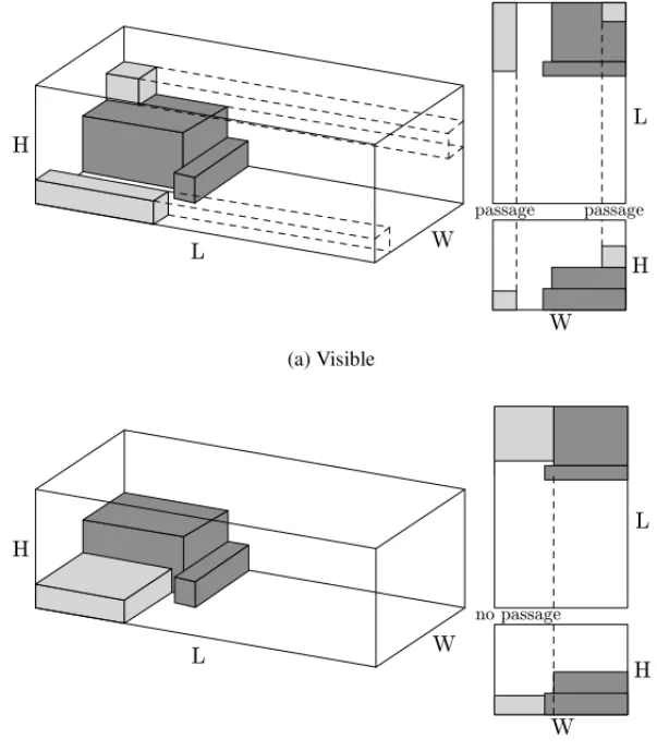
• Boxes that are visible

There has to be a passage from the box to an entrance of the container, that is, the boxes to be unloaded at a destination have to be completely visible from one or more sides of the container in the destination point, or be blocked only by boxes for the same destination. In most of the papers this condition has to be satisfied from the unloading door and from the top of the container. Several authors use this definition, for instance Gendreau et al. [21], Christensen & Rousoe [12], and Ceschia & Schaerf [10]. When a customer is visited, none of the corresponding boxes may be stacked beneath nor be blocked by boxes for customers that are to be visited later. This constraint is violated if for any pair of boxes

i and j such thati has to be unloaded before than j,j is on top ofi(i.e. the base of j is higher than the top ofi and they overlap horizontally), or j is in front ofi(i.e. the back of j is in front of the front ofi, and they overlap across the container). This case reflects the unloading of boxes by forklifts, where they are first elevated and then moved towards the unloading door, as can be seen in Figure 1, in which the boxes for the next costumer appear in light grey color.

L H

W

L

H

W

passage passage

(a) Visible

L H

W

L

H

W

no passage

(b) Not visible

Ltouchable

Htouchable

L

H

W

L

H

W

passage passage

(a) Visible and touchable

Untouchable

L H

W

L

H

W no passage passage

(b) Not visible or not touchable

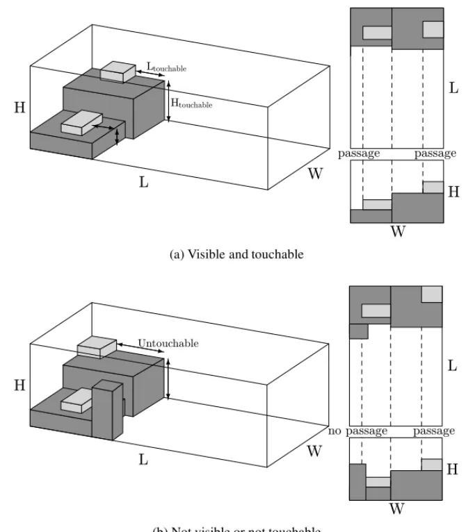
Figure 2– Applying the visible and touchable criterion.

• Boxes that are touchable

For the delivery person to be able to touch item bi with his/her hands, Lt ouchable and Ht ouchablehave to satisfy the following constraints:

Lt ouchable+Ht ouchable≤200

Lt ouchable≤min{200−zi,60}

whereziis the height at which the box is placed (see Fig. 2). Ceschia et al. [11] use only

one parameter, the horizontal distance. Lt ouchableis the distance along the axisLfrom the

box to the nearest place we can use to reach the box.

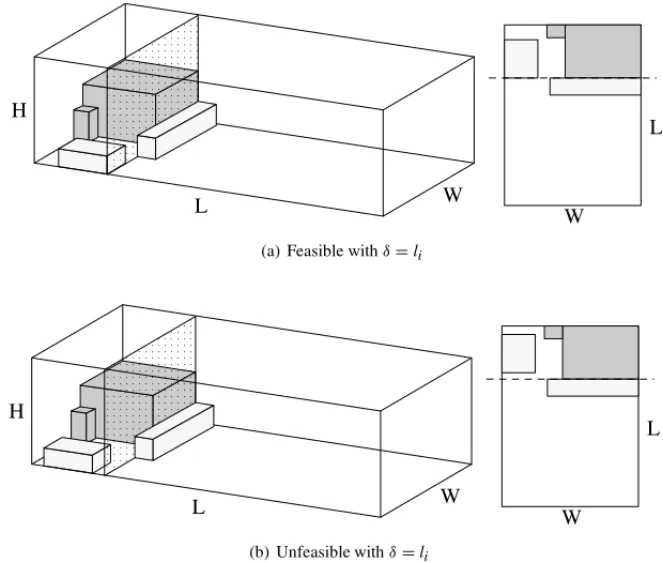
• Boxes that are separated from those of other customers

Junqueira et al. [30] define reachability as a function of a parameter δ, which indicates how many units of length beyond the “border” between boxes of consecutive destinations the worker is allowed to go in order to unload the boxes. They define the “border” as a virtual wall defined after all boxes for a destination have been packed inside the container. These walls separate the boxes for each customer across the length of the container. If this parameterδ =0 (Fig. 3), boxes for the next customer (in light gray) must be completely separated from those for the previous customer (in dark gray). The worker is not allowed to cross this virtual wall. In the general case, the worker is allowed to go only partially beyond the virtual wall. In Figure 4, withδ =li, light gray boxes can be placed beyond

the wall defined by dark gray boxes, but one of their sides must always be on the virtual wall.

L H

W

L

W

(a) Feasible withδ=0

L H

W

L

W

(b) Unfeasible withδ=0

L H

W

L

W

(a) Feasible withδ=li

L H

W

L

W

(b) Unfeasible withδ=li

Figure 4–Applying the Junqueira et al. virtual walls withδ=li.

In these problems in which we have several clients, there is another question to be addressed: can we load boxes for client jbefore all the boxes for a previous clientihave been packed? We can have two cases:

• Restricted

We have to pack the complete shipment for each customer in the given order. That is, it is not possible to pack some boxes for customer j unless all the boxes for customer i

have been packed(j > i). This is the most common circumstance when packing with multi-drop constraints (Christensen & Rousoe [12], Ceschia & Schaerf [10]).

• Unrestricted

In this case, it is possible to pack boxes for customer jeven though there are some boxes for customeri which have been left unpacked (j > i). In this case these boxes would be left out of the loading. In Liu et al. [33] and in Junqueira et al. [30], the objective is to maximize the total volume packed, and this can be achieved by leaving out boxes for several customers.

value 10, while in Figure 5(c) we see the optimal solution packing all the boxes for clients 1 and 3, with value 11, but leaving out the intermediate client 2. Finally, in Figure 5(d) we can see the optimal solution for the less constrained case, with value 12, packing some, but not all, of the boxes for the three clients.

1 1

2 2

3 3 3

(a) Pieces

1

1 2

0 1 2 3 4 5 6 1

2

(b) Restricted

1 1 3

3 3 0 1 2 3 4 5 6 1

2

(c) Unrestricted I

1

1 2

3 0 1 2 3 4 5 6 1

2

(d) Unrestricted II

Figure 5– Packing different subsets of clients’ boxes.

4 PROBLEM DESCRIPTION

We have a container of dimensions (L,W,H) that has to be filled with a set ofnboxes,Bi,i= 1, . . . ,n. Each box has dimensions (li, wi,hi) in cm. and weightwi in kg. and a destination or

drop numberdi. The objective is to find an orthogonal packing of the boxes so as to maximize

the container volume utilization, subject to these constraints:

• Full support:

The base of each box has to be placed on the floor of the container or completely on top of other boxes.

• Allowed orientation:

Each box has a set of allowed orientations due to its content or its structure. The orien-tations are denoted byoi j, wherei = 1, . . . ,n represents the box and j = 1,2,3 the

orientation, that is, the dimension of the box that can be placed upright:oi1=1 if dimen-sionl of boxi can be upright and 0 if it may not,oi2=1 if dimensionwcan be upright and 0 if it may not, andoi3=1 if dimensionhcan be upright and 0 if it may not. At least one of these parameters must be 1 for each boxi.

• Load-bearing strength:

Each box placed in one allowed orientation can bear a maximum weightmi j on top of it,

transmitted downwards onto the boxes supporting it from below. In practice, it depends on the stiffness of the supporting surface: the more rigid it is, the more the weight is spread over the whole surface. When using soft materials like cardboard, the weight of the box above is essentially transmitted down onto the contact area only. We will assume this latter situation and therefore when a boxkis put on top of another boxi, its weightwkwill be divided by its base area to calculate the pressure, pk in gr/cm2, exerted on the

support-ing box. If this pressure pkexceeds the load-bearing capacity of the box below,mi j, the packing is not feasible. Otherwise, the remaining load-bearing capacity of boxi will be reduced bypk.

• Multi-drop:

We admit the three possible definitions of multi-drop constraints described in the previ-ous section. We have designed an algorithm able to deal with all kinds of multi-drop con-straints. Depending on the type of constraint being considered, some steps of the algorithm will be changed, as will be explained in the next section.

5 A GRASP ALGORITHM

The GRASP algorithm was developed by Feo & Resende [16] to solve hard combinatorial prob-lems. For an updated introduction, see Resende & Ribeiro [46]. GRASP is an iterative procedure combining a constructive phase and an improvement phase. In the constructive phase, a solution is built step by step, adding elements to a partial solution. The constructive phase is iterative, greedy, randomized, and adaptive. In the next subsections we describe a constructive procedure, a randomization strategy which will be embedded in the constructive process, some movements for the improvement phase, and a diversification phase which can be included in the iterative structure.

5.1 Constructive Algorithm

The basis of our constructive algorithm is the constructive procedure proposed by Parre˜no et al. [41] for the container loading problem. The algorithm works on maximal spaces. As the selected box is packed into a new space, three new maximal spaces are created. The constructive algorithm uses an updated list of maximal spaces and a list of boxes for the current client still to be packed. The most difficult part in this case is the management of the empty spaces when all the boxes for a client have been packed. In this case, before starting to pack the boxes for the next client, some spaces have to be removed from the list and others have to be updated in order to satisfy the multi-drop constraints. The details of the algorithm can be found in [41]. For completeness we will outline its main steps here.

Step 0: Initialization

S _{=the list of empty maximal spaces created when packing the boxes. Initially,}S _{is just the} empty container.

Step 1: Choosing the maximal space fromS

We have a listS_{of empty maximal spaces, which are the largest empty parallelepipeds} avail-able to be filled with boxes. We use two alternative strategies to choose the maximal space. We alternate between choosing the maximal space with the minimum distance to the back of the container and choosing the maximal space with the largest coordinatez. The reason behind these strategies is to fill the back of the container first or to pile boxes forming stacks.

Step 2: Choosing the boxes to pack

Once a maximal spaceShas been chosen, we consider the remaining boxes of the current cus-tomer fitting intoSin order to choose which one to pack. If there are several boxes of the same dimensions, we consider the possibility of packing a block, that is, packing several of these boxes arranged in a rectangular array with several rows and columns.

Two criteria have been considered to select the configuration of boxes:

1. Best-Volume:

The box or block producing the largest increase in the volume occupied by boxes.

2. Best-Fit:

The box or block which best fits into the maximal space. We compute the distance from each side of the box or block to each side of the maximal space and put these distances in a vector in non-decreasing order. The box or block is chosen using the lexicographical order.

If we are using the visibility criterion, the corner into which the box or the block is packed is the corner of the maximal space with the shortest distance to the origin of the container. In the other two cases, we have to check how and where we put the box or the block in order to make it reachable, always trying to put it as far back as possible so as to maximize the remaining usable space.

Step 3: Updating the listS_{for the current customer}

Unless the box or block fits exactly into spaceS, packing it produces new empty maximal spaces which will replaceS in the listS_{. Moreover, as the maximal spaces are not disjoint, the box or} block being packed can intersect with other maximal spaces which will have to be reduced.

Once the new spaces have been added and some of the existing ones modified, we check the list and eliminate possible inclusions. The listB_{is also updated and the maximal spaces that cannot} accommodate any of the boxes still to be packed are eliminated fromS_{. If}S_{= ∅or}B_{= ∅, the} procedure ends. Otherwise, if we have not finished packing the boxes for the current customer, we go back to Step 1.

Step 4. Updating the listS_{for a new customer}

• Visible: We have to remove from the list all the maximal spaces that are not completely visible from the front of the container. We update the maximal spaces that have some part that is visible and other non-visible.

• Touchable and visible: Apart from the spaces removed when applying the previous crite-rion, we have to remove or update all the spaces that are not touchable.

• Separated: If we work with virtual walls separating the customers and a given value ofδ, we have to remove or update all the maximal spaces whosex-coordinate is lower than the position of the virtual wall minusδ.

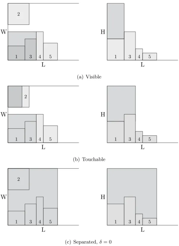
Figure 6 shows an example of the different ways of updating the maximal spaces when the boxes for a client have been packed. The left part of the figure shows the view from the top and the right part the view from one side. Boxes 1 to 5, corresponding to the first customer, have been packed. Using the first criterion, visibility, the space on the floor behind piece 4 cannot be used, and neither can the space on top of piece 1, because piece 3 is taller. Using the second criterion, touchability, the space above piece 3 cannot be reached. Also, as piece 2 is very high, only part of the space above it is touchable. The third criterion, separation withδ =0, builds a virtual wall at the right-hand side of the last piece and this wall cannot be penetrated to pack the next customer’s boxes.

As in Parre˜no et al. [41], two criteria have been considered to select the configuration of boxes:

• The block of boxes producing the largest increase in the objective function. This is a greedy criterion in which the space is filled with the block producing the largest increase in the volume occupied by boxes.

• The block of boxes which fits best into the maximal space. We compute the distance from each side of the block to each side of the maximal space, order these distances in a vector in lexicographical order, and select the block with the minimum distance.

5.2 Randomization

For each type of box and each allowed orientation, a block is built, according to the criterion se-lected. From the set of all possible blocks, a restricted candidate list (RCL) is built and the block to be packed is randomly selected from this list. We have used a value-based Restricted Candi-date List: the candiCandi-dates are selected according to their quality. If the value of the candiCandi-date’s objective function is better than a threshold, the candidate is placed on the list. In the course of the process of building blocks we getCminandCmax, the largest and the smallest values of all the candidates, and the value of each candidateC. The candidate is accepted into theRCL

if it satisfiesC ≥ Cmin+γ (Cmax−Cmin). The parameterγ ∈ [0,1] controls the size of the list. Ifγ =0, all the blocks go into the list and the selection is completely random. In contrast,

W

L 1 3 4 5

2

L H

1 3 4 5

(a) Visible

W

L 1 3 4 5

2

L H

1 3 4 5

(b) Touchable

W

L 1 3 4 5

2

L H

1 3 4 5

(c) Separated,δ= 0

Figure 6– Updating the maximal spaces after packing the boxes for a client.

chosen. For 0< γ <1, the number of blocks going into the list is not predefined, but it depends on the relative values of the candidates.

We also randomize the criterion used to assign a value to each block. At each iteration, we choose at random between the criterion based on the increase in the occupied volume and the criterion based on the way in which the blocks fit into the space, and build the solution using the criterion chosen.

5.3 Improvements

• The first movement consists of eliminating the lastk% boxes packed in the complete so-lution (for instance, the last 50%). We choose the valuek at random from the interval [30,90]. The removed items plus the items that were left unpacked in the solution are then packed again using the deterministic constructive procedure. In this call of the determin-istic algorithm we can use the objective function Best-Volume or the objective function Best-Fit. Both alternatives have been tested and their results will appear in the next sec-tion. We consider that a solution has improved if the total volume of the packed boxes has increased.

• In the second improvement, we apply the previous procedure to the partial solution we have when we finish packing the boxes for a customer. In this case, we consider that the solution has improved if the area occupied by the partial solution has decreased.

The improvement phase is only called if the solution of the constructive phase is considered to be promising, that is, if it is considered a good starting point for improving on the best known solution. Therefore, we only consider those solutions that are above a certain threshold. At the beginning, the threshold takes the value of the first solution of the constructive algorithm. Then, if at an iteration the solution value is greater than the threshold, we update this threshold to this value and go to the improvement phase. If the solution value is lower than the thresh-old, the solution is not improved and the reject counter (nit er) is increased. When the number of rejected solutions is greater than a value maxFilter, the threshold is decreased according to the expression:

t hreshold =t hreshold−λ(1+t hreshold)

whereλis set at 0.2 andmax Filt er =5, as in Marti & Moreno [36].

5.4 Memory-based constructive phase

When we deal with the unrestrictive variant of the problem we can modify the constructive phase. In this case it is possible not to pack some boxes for a customer or even not to pack all the boxes for one or more customers and continue with the packing for the following customers. This will give us more flexibility which could lead to better solutions.

We save the information relative to the area of the floor of the container used by the partial solution each time the packing of the boxes for a customer is finished. Every I t erm iterations

(which we fixed at 500), we compute for each customer the difference between the area used before and after their packing is done and divide it by the total volume of their boxes. The average value of this ratio gives us an estimate of the relative cost of packing the boxes for this customer and we use this information to decide which customers and boxes can be left out of the packing in order to explore possibly better solutions.

For the next I t err iterations, before starting the loading process, we remove from the list of boxes a percentage of boxes to be packed (I t err =max{5∗cust omers,250}). The percentage

from the interval(0.3∗(T ot V ol−V ol Best),0.7∗(T ot V ol−V ol Best)), whereT ot V olis the total volume of the boxes to pack andV ol Best the volume of the boxes in the best known solution. We take the customer with the greatest ratio and remove boxes randomly until we reach the predefined percentage. If we do not reach the percentage with this customer, we take the customer with the next largest value, and so on. The differenceT ot V ol−V ol Bestindicates the volume of the boxes left unpacked in the best known solution. We want to make room for boxes at the end of the list, eliminating boxes of previous costumers, but ensuring that the reduced list is large enough to fill completely the container.

6 Computational results

The algorithm was coded in C++ and run on an Intel Core i7-2600 CPU with 3.40 GHz and 12 GB of RAM. We used several types of test instances. First, we used the test problems generated by Bischoff & Ratcliff [5]. The 700 problems are divided into 7 classes(B R1, . . . ,B R7)of 100 in-stances each. The number of box types in each class ranges from 3 different types in the first class to 20 types in the seventh class. This set of 700 instances has been used by many authors and is therefore the most usual benchmark for comparing the algorithms. In these instances the boxes have been generated independently of the container dimensions, so there is no guarantee that all the boxes of one instance will fit into the container. The weight of each box is proportional to its volume and the load-bearing limits have been drawn randomly from a uniform distribu-tion. The problems are available on the ESICUP website: http://paginas.fe.up.pt/∼esicup/tiki-list file gallery.php?galleryId=4. To extend these data sets for the multi-drop problem, Chris-tensen & Rousoe [12] take a number of customers 2, 5, 10, or 50, and assign each box at random to one of these customers. The assignment is done independently for each number of customers.

We have also used other sets of instances in order to compare with other authors. We compare our algorithm with the exact procedure developed by Junqueira et al. [30] using the 16 instances they generated. We also use the instances by Ceschia & Schaerf [10] in which they pack a single container. Finally, in order to compare with the procedure by Liu et al. [33], we have generated 100 instances using the information provided in their paper.

For a last comparison with algorithms only considering load-bearing constraints, we have ex-tended the study to classes BR8-BR15 of strongly heterogeneous instances, also developed by Bischoff & Ratcliff [5]. In these classes, the number of box types ranges from 30 for BR8 to 100 for BR15.

For our GRASP algorithm we have set a maximum number of 50000 iterations. In all the tables the averages correspond to the percentage of volume used.

6.1 Comparing with Ceschia & Schaerf [10]

made of homogeneous blocks of boxes. The boxes are ordered by drop number and the way in which they are packed ensures that the multi-drop constraints are satisfied. A local search im-proves the solution by changing the sequence of boxes, but respecting the multi-drop conditions.

In their computational results, they use a set of 117 real-world problems, some of them involv-ing just one container and others involvinvolv-ing several containers. Here we have used only the 23 instances involving one container. A summary of the results appears in Table 1. The GRASP algorithm matches the reported solutions for 10 instances and improves on the results for the other 13 instances.

Table 1– Comparison with Ceschia & Schaerf [10] on instances with one container.

GRASP Ceschia & Schaerf

Average volume (%) 75,04 70,04

Average CPU time (seconds) 18,66 39.41

6.2 Comparing with Christensen & Rousoe [12]

Christensen & Rousoe [12] considered the version of the multi-drop constraints in which a box can be unloaded if it is visible from the top and from the door of the container. They also included orientation, full support and load-bearing, developed a tree-search algorithm, and tested it on the Bischoff & Ratcliff [5] instances. Their algorithm was implemented in C++ and the tests were performed on a Linux machine with 2.4 GHz 64 bit AMD processor and 2 GB RAM, with a time limit of 60 seconds.

In Table 2 we can see the results of our algorithm compared with the Christensen & Rousoe [12] algorithm. The table shows that our algorithm obtains better solutions for any number of cus-tomers, from the classic problem with just one customer to problems with large numbers of customers, with similar running times. Table 2 also shows that the solution quality depends not only on the number of customers, but also on the combination of the number of box types and the number of customers in the problem. When there are only three box types (BR1) the solution quality only drops 13% when going from 1 to 50 customers, but in the case of 20 box types (BR7) the difference between 1 and 50 customers is almost 30%. It is not surprising that the difficult problems have many customers and many box types.

6.3 Comparing with Liu et al. [33] and with Jin et al. [29]

Table 2– Comparison with Christensen & Rousoe [12].

Customers GRASP Christensen

BR1 BR2 BR3 BR4 BR5 BR6 BR7 Average & Rousoe

1 92,47 92,75 92,76 92,22 91,68 91,01 89,62 91,79 89,07

2 91,77 90,76 89,47 88,56 87,78 86,69 85,51 88,65 85,96

5 88,56 86,02 83,15 81,36 80,14 78,30 76,12 81,95 78,52

10 85,28 81,43 77,82 76,14 74,47 72,45 70,22 76,83 72,64

50 79,32 73,96 68,98 66,87 64,85 63,25 60,61 68,26 64,45 Average 87,48 84,98 82,44 81,03 79,78 78,34 76,42 81,50 78,13

Time 30,29 34,01 37,93 41,98 57,18 63,35 69,94 47,81 60

be packed. As a particular case, they developed algorithm SIBP for a fixed box ordering. Liu et al. [33] tested the SIBP algorithm and found that it did not guarantee the multi-drop constraints. Then, in order to compare with their algorithms, they used algorithm SIBP’, an adapted version of SIBP satisfying the multi-drop constraints. For the tests they used the 100 instances of set BR7 ([5]), adding a random order to the original boxes. Algorithms were run 100000 times on each instance and average results were reported, using an Intel Core 2 Duo E8400 3.00 GHz PC with 2.00 GB of memory.

We have generated 100 instances following the information provided in their paper, because their original data are unavailable. However, given that their data set has 100 problems and that we report only averages, it is unlikely to introduce any systematic bias in the results.

Table 3 shows that the our GRASP algorithm is able to obtain better results even for this special case of multi-drop constraints in similar computing times.

Table 3– Comparison with Liu et al. [33] and Jin et al. [29].

Restrictive case Unrestrictive case

GRASP SBIP’ A1 GRASP A2

Average 49,52 34.17 48,78 53.27 53.18 Time 84,11 63,76 51,98 82.14 85.68

6.4 Comparing with Junqueira et al. [30]

We have also compared our GRASP algorithm with the exact algorithm by Junqueira et al. [30]. We compare with this type of problem for two reasons. First, because they deal with a different type of multi-drop constraint. As explained in Section 3, they separate the boxes for each cus-tomer using virtual walls and boxes can only be unloaded if there are less than a given valueδ

Table 4– Comparison with Junqueira et al. [30],δ=li.

δ=li

Number Box Container % Volume packed of boxes types length Junqueira et al. GRASP

A1 20 1 15 100 100

A5 41 5 15 100 100

41 5 12 90 100

A10 99 10 15 100 100

A20 89 20 15 100 100

B1 50 1 15 100 100

B5 813 5 15 100 100

B10 1000 10 15 100 100

B20 674 20 15 100 100

Table 5– Comparison with Junqueira et al. [30],δ=0.

δ=0 Number Box Container % Volume packed of boxes types length Junqueira et al. GRASP

A1 20 1 15 100 100

20 1 12 95 95

A5 41 5 15 100 100

41 5 12 77,9 95,5

A10 99 10 15 100 100

A20 89 20 15 100 100

89 20 12 92,8 98,4

B1 50 1 15 100 100

B5 813 5 15 100 100

B10 1000 10 15 100 100

B20 674 20 15 100 100

They generated a set of instances with different numbers of boxes. The number of customers was set to three for all the problems. Two values of the parameterδ, defining when the boxes are available, were used,δ =0 andδ =li. Their tests were performed on a PC Core i7 (2.8 GHz, 8.0 GB) with a time limit of 3600 seconds.

Tables 4 and 5 show the results obtained consideringδ = li and δ = 0, respectively. The

problems in Table 4, withδ = li, are less restricted and both algorithms are able to pack all the boxes. Whenδ =0, in Table 5, the problems are more restricted and in some instances their exact algorithm fails to obtain the optimal solution within the time limit of 3600 seconds. In these cases, our GRASP algorithm is able to obtain equal or better solutions.

6.5 Problems with only one customer and load bearing constraints

Table 6– Comparing with Alonso et al. [1].

Class GRASP Alonso et al. Class GRASP Alonso et al.

BR1 82,5 81,4 BR8 83,7 85,5

BR2 86,7 85,7 BR9 82,4 84,8

BR3 88,4 87,3 BR10 81,4 84,0

BR4 88,1 86,9 BR11 80,1 82,8

BR5 87,4 86,6 BR12 78,9 81,3

BR6 86,9 86,3 BR13 77,7 80,2

BR7 85,53 85,7 BR14 76,6 78,9

BR15 75,5 78,0

Average (1-7) 86,5 85,7 Average (8-15) 79,5 83,7 Time (sec.) 13,5 9,8 Time (sec.) 102,8 64,7 Average(1-15) 82,8 83,5

by Alonso et al. [1] which has obtained the best results for this type of problem, and use the same test instances. In this case there is only one customer for the complete shipment. They proposed a GRASP algorithm with different the two algorithms can be seen in Table 6. In the first seven classes the new algorithm obtains better results, but for more heterogeneous instances the Alonso et al. [1] algorithm is better. On average, the results obtained by our algorithm can be considered competitive also for instances without multi-drop constraints.

7 CONCLUSIONS

We have reviewed different algorithms and types of multi-drop problems. We have developed a GRASP algorithm with a new constructive procedure and some new improvement movements. The main contribution is that this algorithm is able to accommodate the different versions of the multi-drop constraints which have appeared in the literature and it obtains very good results compared with existing heuristics for the different versions of the problem. The algorithm also gets good results for other variants of the problem including full support and load-bearing con-straints, even when all the boxes are for the same customer.

The algorithm is flexible and could be adapted to other constraints, such as the maximum weight of the container, weight distribution, and boxes in which the weight is not proportional to the volume. In the near future we plan to use this algorithm to work with more practical situations, such as those combining loading and routing problems.

ACKNOWLEDGEMENTS

The authors would like to thank Soren Christensen and Leonardo Junqueira, who kindly sent us the sets of instances used in their papers.

REFERENCES

[1] ALONSO MT, ALVAREZ-VALDESR, PARRENO˜ F & TAMARITJM. 2014. A Reactive GRASP algorithm for the container loading problem with load-bearing constraints.European Journal of Industrial Engineering,8(5): 669–694.

[2] ARAUJOOCB & ARMENTANOVA. 2007. A multi-start random constructive heuristic for the con-tainer loading problem.Pesquisa Operacional,27: 311–331.

[3] BISCHOFFEE. 2006. Three-dimensional packing of items with limited load bearing strength. Euro-pean Journal of Operational Research,168: 952–966.

[4] BISCHOFFEE & MARRIOTTMD. 1990. A comparative evaluation of heuristics for container load-ing.European Journal of Operational Research,44(2): 267–276.

[5] BISCHOFFEE & RATCLIFFMSW. 1995. Issues in the development of approaches to container load-ing.Omega,23: 377–390.

[6] BORTFELDTA. 2012. A hybrid algorithm for the capacitated vehicle routing problem with three-dimensional loading constraints.Computers and Operations Research,39(9): 2248–2257.

[7] BORTFELDTA & GEHRINGH. 2001. A hybrid genetic algorithm for the container loading problem.

European Journal of Operational Research,131: 143–161.

[8] BORTFELDTA, GEHRING H & MACKD. 2003. A parallel tabu search algorithm for solving the container loading problem.Parallel Computing,29(5): 641–662.

[9] BORTFELDTA & W ¨ASCHERG. 2013. Constraints in container loading – A state-of-the-art review.

European Journal of Operational Research,229(1): 1–20.

[10] CESCHIAS & SCHAERFA. 2013. Local search for a multi-drop multi-container loading problem.

Journal of Heuristics,19: 275–294.

[11] CESCHIAS, SCHAERFA & STUTZLE¨ T. 2013. Local search techniques for a routing-packing prob-lem.Computers and Industrial Engineering,66(4): 1138–1149.

[12] CHRISTENSENSG & ROUSOEDM. 2009. Container loading with multidrop constraints. Interna-tional Transactions in OperaInterna-tional Research,16(6): 727–743.

[13] DOERNERKF, FUELLERERG, GRONALTM, HARTLRF & IORIM. 2007. Metaheuristics for the vehicle routing problem with loading constraints.Networks,49: 294–307.

[14] EGEBLADJ, GARAVELLIC, LISIS & PISINGERD. 2010. Heuristics for container loading of furni-ture.European Journal of Operational Research,200(3): 881–892.

[15] ELEY M. 2002. Solving container loading problems by block arrangement.European Journal of Operational Research,141: 393–409.

[16] FEOT & RESENDEMGC. 1989. A Probabilistic Heuristic for a Computationally Difficult Set Cov-ering Problem.Operations Research Letters,8: 67–71.

[17] FANSLAUT & BORTFELDT A. 2010. A tree search algorithm for solving the container loading problem.INFORMS Journal of Computing,22: 222–235.

[18] FEKETESP, SCHEPERSJ & VANDERVEENJC. 2007. An exact algorithm for higher-dimensional orthogonal packing.Operations Research,55: 569–587.

[19] GEHRINGH & BORTFELDTA. 1997. A genetic algorithm for solving the container loading problem.

[20] GEHRINGH & BORTFELDTA. 2002. A parallel genetic algorithm for solving the container loading problem.International Transactions in Operational Research,9: 497–511.

[21] GENDREAUM, IORIM, LAPORTEG & MARTELLOS. 2006. A tabu search algorithm for a routing and container loading problem.Transportation Science,40(3): 342–350.

[22] GENDREAUM, IORIM, LAPORTEG & MARTELLOS. 2008. A Tabu search heuristic for the Vehicle Routing Problem with two-dimensional loading constraints.Networks,51(1): 4–18.

[23] GEORGEJA & ROBINSONDF. 1980. A heuristic for packing boxes into a container.Computers and Operations Research,7(3): 147–156.

[24] GILMOREPC & GOMORYRE. 1965. Multistage cutting stock problems of two and more dimen-sions.Operations Research,13: 94–120.

[25] HAESSLERRW & TALBOTFB. 1990. Load planning for shipments of low density products. Euro-pean Journal of Operational Research,44(2): 289–299.

[26] HIFIM. 2002. Approximate algorithms for the container loading problem.International Transactions in Operational Research,9(6): 747–774.

[27] IORIM, SALAZARJJ & VIGOD. 2007. An Exact Approach for the Vehicle Routing Problem with Two-Dimensional Loading Constraints.Transportation Science,41: 253–264.

[28] IORIM & MARTELLOS. 2010. Routing problems with loading constraints.TOP,18: 4–27. [29] JINZ, OHNOK & DUJ. 2004. An efficient approach for the three-dimensional container packing

problem with practical constraints.Asia-Pacific Journal of Operational Research,21(3): 279–295. [30] JUNQUEIRAL, MORABITOR & YAMASHITADS. 2012. MIP-based approaches for the container

loading problem with multi-drop constraints.Annals of Operations Research,199(1): 51–75. [31] JUNQUEIRAL, MORABITOR & YAMASHITADS. 2012. Three-dimensional container loading

mod-els with cargo stability and load bearing constraints.Computers and Operations Research,39: 74–85. [32] LAIKK, XUEJ & XUB. 1998. Container packing in a multi-customer delivering operation.

Com-puters and Industrial Engineering,35(1–2): 323–326.

[33] LIUWY, LINCC & YUCS. 2011. On the three-dimensional container packing problem under home delivery service.Asia-Pacific Journal of Operational Research,28(5): 601–621.

[34] MACKD, BORTFELDTA & GEHRINGH. 2004. A parallel hybrid local search algorithm for the container loading problem.International Transactions in Operational Research,11(5): 511–533. [35] MARTELLOS, PISINGERD & VIGOD. 2000. The three-dimensional bin packing problem.

Opera-tions Research,48(2): 256–267.

[36] MARTI R & MORENO-VEGA JM. 2003. Metodos multiarranque. Inteligencia Artificial, 19(2): 49–60.

[37] MORABITOR& ARENALESM. 1994. An AND/OR-graph approach to the container loading prob-lem.International Transactions in Operational Research,1(1): 59–73.

[38] MOURA A & OLIVEIRA JF. 2005. A GRASP approach to the container loading problem.IEEE Intelligent Systems,20: 50–57.

[40] PARRENO˜ F, ALVAREZ-VALDESR, OLIVEIRAJF & TAMARITJM. 2008. A Maximal-Space Algo-rithm for the Container Loading Problem.INFORMS Journal on Computing,20(3): 412–422. [41] PARRENO˜ F, ALVAREZ-VALDESR, OLIVEIRAJF & TAMARITJM. 2010. Neighborhood structures

for the container loading problem: A VNS implementation.Journal of Heuristics,16: 1–22. [42] PARRENO˜ F, ALVAREZ-VALDESR, OLIVEIRAJF & TAMARITJM. 2010. A hybrid GRASP/VND

algorithm for two- and three-dimensional bin packing.Annals of Operations Research, 179(1): 203–220.

[43] PISINGERD. 2002. Heuristics for the container loading problem.European Journal of Operational Research,141(2): 382–392.

[44] RATCLIFFMSW & BISCHOFFEE. 1998. Allowing for weight considerations in container loading.

OR Spectrum,20: 65–71.

[45] RENJ, TIANY & SAWARAGIT. 2011. A tree search method for the container loading problem with shipment priority.European Journal of Operational Research,214(3): 526–535.

[46] RESENDE MGC & RIBEIRO CC. 2003. Greedy Randomized Adaptive Search Procedures. In: GLOVERF & KOCHENBERGERG (editors),Handbook of Metaheuristics, pages 219–249, Kluwer, Boston.

[47] TERNOJ, SCHEITHAUERG, SOMMERWEISS& RIEHMEJ. 2000. An efficient approach for the multi-pallet loading problem.European Journal of Operational Research,123: 372–381.

[48] W ¨ASCHERG, HAUSSNERH & SCHUMANNH. 2007. An improved typology of cutting and packing problems.European Journal of Operational Research,183(3): 1109–1130.