LIST OF SYMBOLS AND ACRONYMS DASC Time-delayed anti-swing controller
FHL Force transferred from the load to the helicopter kd Gain of the delayed feedback controller L Load cable length
mL Load mass
MHL Moment transferred from the load to the helicopter N Number of particles in the PSO
PSO Particle swarm optimization algorithm RH Hook position vector
RL Load position vector p,q,r Helicopter angular velocities Vmax Maximum velocity of PSO u,v,w Helicopter velocities
x,y,z Helicopter center of gravity position I,ș,ȥ Euler angles
IL,șL Load swing angles IJd Time delay
Ȗ1,Ȗ2 PSO learning factors
INTRODUCTION
Helicopters can be used for carrying heavy loads in civil, military, and rescue operations, where the use of ground-based equipment would be impractical or impossible. In these applications, the external load behaves like a pendulum. If the pendulous motion of the load exceeds certain limits, it may damage the load or threaten the life of the rescued person. Moreover, the external load can change natural frequencies and mode shapes of the low frequency modes of the heli-copter. In addition, the aerodynamics of the load may make LWXQVWDEOHLQFHUWDLQÀLJKWFRQGLWLRQV7KHVHSUREOHPVVORZ or even prevent an accurate pickup or placement of the load. Furthermore, it adds extra effort on the pilot.
The dynamics of a helicopter with external suspended loads received considerable attention in the late 1960s and early 1970s. Two reasons for this interest were the extensive external load operations in the Vietnam War, and the heavy-lift helicopter program (HLH). Such concern has been renewed recently with the advances in the modern control technologies (Bisgaard et al., 2006).
Many efforts were done for modeling the slung load and studying its effect on the helicopter dynamics; however, there are relatively few works that discussed the swing control of the helicopter slung (Cicolani and Kanning, 1992). One of WKH¿UVWLQYHVWLJDWLRQVLQWRDXWRPDWLFFRQWUROIRUKHOLFRSWHUV with slung loads was conducted by Wolkovitch and Johnston (1965). The single-cable dynamic model was developed in a straightforward application of the Lagrange equations.
Anti-swing Controller Based on Time-delayed Feedback for
Helicopter Slung Load System near Hover
Hanafy Mohammad Omar*
Qassim University - Buraydah – Saudi Arabia
Abstract: ,Q tKLV paper, a Qew aQtLVwLQJ FRQtrRller IRr KelLFRpter VluQJ lRad VyVtem Qear KRver ÀLJKt LV prRpRVed. 7KLV FRQtrRller LV EaVed RQ tLmedelayed IeedEaFk RI tKe lRad VwLQJ aQJleV. 7Ke Rutput IrRm tKLV FRQtrRller LV addLtLRQal displacement that was added to the helicopter trajectory in the longitudinal and lateral directions. Hence, its implementa-tion is simple and it only needs a small modi¿caimplementa-tion to the soItware oI helicopter posiimplementa-tion controller. 7he parameters oI the controllers are determined using the method of particle swarms by minimizing an index, which is a function of the load swing history. 7he simulation results show the effectiveness of the proposed controller in suppressing the swing of the suspended load and the stabilization of the helicopter.
Keywords: Helicopter, Slung load, Particle swarms, Swing.
Received: 10/03/12 Accepted: 13/05/12 *author for correspondence: [email protected]
Abzug (1970) later expanded on this model to consider the case of two tandem cables. However, his formulation was based on the Newton-Euler equations of motion for small perturbations, separated into longitudinal and lateral sets. Aerodynamic forces on the cables and the load were neglected, as were the rotor dynamic modes.
Briczinski and Karas (1971) involved the computerized simulation of a helicopter and external load in real time with a pilot in the loop. Load aerodynamics was incorporated into the model, as well as rotor-downwash effects in the hover.
Asseo and Whitbeck (1973) on their paper on the control requirements for slung-load stabilization used the linearized equations of motion of the helicopter, winch, cable, and load for variable suspension geometry and then used them in conjunction with modern control theory to design several control systems for each type of suspension.
Cera and Farmer (1974) examined the feasibility of stabi-OL]LQJH[WHUQDOORDGVE\PHDQVRIFRQWUROODEOH¿QVDWWDFKHG to the cargo. In their simple linear model representing the yawing and the pendulous oscillations of the slung-load system, it was assumed that the helicopter motion was unaf-fected by the load.
Raz et al. (1989) investigated the use of an active aerodynamic load stabilization system for a helicopter slung-load system.
All these studies are based on the classical control techniques. In this paper, a new anti-swing controller for heli-FRSWHUVOXQJORDGV\VWHPQHDUKRYHUÀLJKWLVXVHG,WLVEDVHG on time-delayed feedback of the load swing angles (Masoud et al., 2002, Omar and Nayfeh, 2005). The output from this controller was additional displacements that are added to the helicopter trajectory in the longitudinal and lateral directions. Hence, its implementation is simple and it just needed small PRGL¿FDWLRQWRWKHVRIWZDUHRIKHOLFRSWHUSRVLWLRQFRQWUROOHU The parameters of the controllers were determined using particle swarms optimization technique by minimizing an index, which is a function of the load swing history.
Particle swarm optimization (PSO) is a population-based stochastic optimization technique, which is inspired by the VRFLDOEHKDYLRURIELUGÀRFNLQJRU¿VKVFKRROLQJ,WVKDUHV many similarities with evolutionary computation techniques, such as genetic algorithms (GA) (Kennedy, 1997). The system is initialized with a population of random solutions and it searches for optima by updating generations. However, unlike GA, the PSO has no evolution operators such as crossover and PXWDWLRQ,Q362WKHSRWHQWLDOVROXWLRQVFDOOHGSDUWLFOHVÀ\ through the problem space by following the current optimum
particles. Compared to GA, the advantages of PSO are that it is easy to implement and there are few parameters to adjust. Moreover, PSO, like all evolutionary algorithms, optimizes a performance index based only on input/output relationships. Therefore, minimal knowledge of the plant under investiga-tion is required. In addiinvestiga-tion, because derivative informainvestiga-tion is not needed in the execution of the algorithm, many pitfalls that gradient search methods suffer can be overcome.
MATHEMATICAL MODEL
The helicopter with a slung system can be considered as a multi-body dynamical one. The motion equations of each ERG\PD\EHZULWWHQVHSDUDWHO\DQGWKHQPRGL¿HGE\DGGLQJ the interaction forces between them (Fusato, 1999, Poli and Cromack, 1973).
Modeling the helicopter
In this study, the helicopter was modeled as a rigid body with six degrees of freedom. With Euler angles, the helicopter states are 12, including translational (u, v, w) and angular velocities (p, q, r), Euler angles (ij, ș, ȥ), and helicopter posi-tion (x, y, z) (Prouty, 2003).
Modeling the slung load
The external load is modeled as a point mass, which behaves like a spherical pendulum suspended from a single point. The cable is assumed to be inelastic and without mass. The geometry and the relevant coordinate systems are shown in Fig. 1. The unit vectors iH , jH , kH of the hook coordinate system always remain parallel to those of the body axis system. The position of the load was described by the two angles șL and ijL, where ijL is a load angle in the xz plane, and
șL is the load oscillation angle out of the xz plane. Therefore,
the position vector RL of the load with respect to the suspen-sion point is given by Eq. 1:
( ) ( ) ( ) ( ) ( )
cos sin sin cos cos
RL=L iL zLiH+L iLjH+L iL zLkH (1)
The position vector RH of the hook with respect to the heli-copter center of gravity (CG) is given by Fusato et al. (1999), as seen in Eq. 2:
FLJXUH&RQ¿JXUDWLRQRIKHOLFRSWHUZLWKDVOXQJORDG
The absolute velocity VL of the load is given by Eq. 3:
VL=Vcg+Ro +X#R (3)
where, V
CGis the absolute velocity of the helicopter mass center, R = RL + RH is the position vector of the load with respect to the helicopter mass center, and
ȍ p iH + q jH+ r kH is the angular velocity of the helicopter.
The absolute acceleration aL of the load is (Eq. 4):
aL=VoL+X#VL (4)
The unit vector in the direction of the gravity force is given by Eq. 5:
( ) ( ) ( ) ( ) ( )
sin sin cos cos cos
Kg=- i iH+ z i jH+ z i kH (5)
Besides the gravity, there is an aerodynamic force applied on the point mass load. Since the analysis in this work was restricted to the helicopter motion near hover, the aerodynamics loads on the load were neglected. The equations of load motion were written by enforcing moment equilibrium on the suspension point, (Eq. 6):
( ) 0
RL# -m aL L+m gkL g = (6)
Equation 6 provides three scalar equations of second orders, only the equations in the x and y directions are retained, which represent the equations of load motion.
Load contributions to helicopter forces
The suspended load introduces additional terms on the rigid body force and moment equations of helicopter motion
(Fig. 2). The force FHL that the load exerts on the helicopter is given by Eq. 7:
FHL=-m aL L+D+m gkL g (7)
The additional moment MHL is therefore given by Eq. 8:
MHL=RH×FHL (8)
Equations 7 and 8 are derived using Mathematica, which gives highly nonlinear expressions. These equations cannot be used for stability analysis. Therefore, they must be linearized around the trim condition. In order to be able to perform the linearization process, the trim values of the helicopter and the load must be determined.
Figure 2. Load contribution to helicopter forces (Fusato et al., 1999).
Linearizing the motion equations
The motion equations obtained were highly nonlinear. We needed to linearize them in order to solve and analyze the helicopter motion. To do that, we used the small-disturbance theory. To apply this theory we assumed that the motion of the helicopter and the load consisted of small deviations about a VWHDG\ÀLJKWFRQGLWLRQ$IWHUDSSO\LQJWKHVPDOOGLVWXUEDQFH theory, we got the helicopter linearized equations of motion.
The obtained equations were nonlinear and complicated. For the design purpose, these equations are linearized about the hovering conditions. Near hover, the forward speed is nearly zero (i.e. uo :HFDQDOVRDVVXPHWKDWWKHKHOLFRSWHU roll angle is also zero even with the effect of the load on the helicopter (I0 ). At this condition, the load trim equations provided the following trim values (Omar, 2005), as in Eq. 9:
0,
Lo Lo o
By imposing such results to the linearized load equations,
ZHZHUHDEOHWR¿QGWKHIROORZLQJHTXDWLRQVRIPRWLRQIRUWKH
load (Eqs. 10 to 12):
[ ] cos[ ] [ ] [ ] [ ] [ ] giLt -g i z0 t +y q tho +V to +LiL t =0
p
(10)
(11)
The forces exerted by the load on the helicopter are:
(12)
The moments in the x-y-z directions are (Eq. 13):
(13) [ ] [ ] [ ] [ ] [ ] [ ] [ ] [ ] [ ] [ ] [ ] [ ] [ ] cos cos sin cos M m
gy t gx t x y p t
Ly p t x y q t y U t x V t
Lx t Ly t
z L
h h h h
h h h h h
h L h L
0 0
0
0
i i i z
i
i i z
=
+ +
- - +
-- +
o
o o o o
p p J L K K K N P O O O [ ] [ ] [ ] [ ] [ ] [ ] [ ] [ ] [ ] [ ] [ ] [ ] [ ] [ ] [ ] [ ] [ ] cos sin sin cos cos sin M m
gz t gx m t x z m p t t
Lz p t x z r t Lx r t z U t
x W t Lz 0 t Lx 0 t
y L
h h L h h L
h h h h h
h h L h L
0 0
0 0
i i i i
i i
i z i z
=
- +
-+ + +
-+ - +
o
o o o o
o p p
J L K K K N P O O O [ ] [ ] [ ] [ ] [ ] [ ] [ ] [ ] [ ] [ ] [ ] [ ] sin cos cos sin M m
gy t gz t y z q t
y z Ly r t z V t y W t
Lz t Ly t
0 0
0
0
x L
h h h h
h h h h h
h L h L
i i i z
i
i i z
=
- - +
- + +
-+
-o
o o o
p p J L K K K ^ N P O O O h
These equations are linear and can be formulated
LQDVWDWHVSDFHIRUP,IZHGH¿QHWKHORDGVWDWHYHFWRUDV
xL L L L L
T z i z i
=6o o @, the load equations in state space can be written as Eq. 14:
E xL =A xL (14)
where,
x is the state vector for the load and the helicopter (i.e., x >xH xL]).
Similarly, the effect of the load on the helicopter force terms can be written also as Eq. 15:
F
M E x A x
HL
HL
HL HL = o+
= G (15)
The linearized equations of helicopter motion and the load can be written in the following state space forms (Eq. 16):
x x
x Ax B
h L h = = + o o o
= G (16)
PROPOSED ANTI-SWING CONTROLLER
7KHFRQ¿JXUDWLRQRIWKHSURSRVHGFRQWUROOHULVVKRZQLQ
Fig. 3. It consists of two control systems: a tracking and an anti-swing one. Helicopter Dynamics Load Dynamics Helicopter States Load Forces
Anti - Swing Controller Load Swing Angles Helicopter Attitude and Position Controller + + Helicopter attitude and position Reference )LJXUH&RQ¿JXUDWLRQRIWKHSURSRVHGDQWLVZLQJFRQWUROOHU
We needed to design a tracking controller for the helicopter to follow the trajectory generated by the anti-swing controller. Therefore, the controller design of the whole system could be
GLYLGHGLQWRWZRVWDJHV,QWKH¿UVWRQHWKHWUDFNLQJFRQWUROOHU
for the helicopter alone was designed by neglecting the effect of the slung load on the helicopter dynamics. The function of this controller is to stabilize the helicopter and to follow the trajectory generated by the anti-swing controller. In the second stage, the whole system is integrated by augmenting the dynamics of the controlled helicopter with the dynamics of the slung load. Then, the proposed anti-swing controller is added to the integrated system, and the performance of the whole system is evaluated. The optimal parameters of the anti-swing controller are determined based on minimizing the history of the load swing.
To design the tracking controller, we assumed that the reference trajectory for the helicopter states is xref, then, the error signal is e=xHref-xH. Using state feedback technique, the helicopter control input can be written as Eq. 17:
( )
K x x
h= Href- H (17)
depends on minimizing a quadratic function that can be writ-ten as Eq. 18:
Indx e QeT TR dt
t
0 f
h h
=
#
^ + h (18)Since the goal was to minimize the error signal, Q is chosen with high gains compared to R. After determining K, the helicopter state space model can be rewritten as Eq. 19:
( )
x A B K x B Kx
A x B x
H H H H H
c H c
= - +
= +
o Href
Href (19)
Equation 19 indicates that the reference states become the new inputs for the helicopter.
In the second stage, the anti-swing controller was designed. After modifying the helicopter dynamics by incorporating the stability and tracking controller, the effect of the load swing forces were added to the state space model in Eq. 16. Before this step, we needed to express Eq. 19 in terms of the total state vector, which include the helicopter and the load states. In this case, the helicopter dynamics can be written as Eq. 20:
(20)
x A x
x B
x
A x B x
0 0 0 H c H L c ref 1 1 = + = +
o 6 @= G 6 @= HrefG
7KHVOXQJORDGHIIHFWPRGL¿HVWKHIRUFHVDQGPRPHQWV
equations in the helicopter equations of motion. Recalling Eq. 16, the forces and moments from the slung load can be written as Eq. 21:
F
M E x A x
HL
HL
HL HL
= o+
= G
(21)
Adding such forces to the helicopter dynamics, the new model can be written as Eq. 22:
(22) [ ] [0] [0] [0] [0] [0] I x x A
A x E x B x
E x A x E x B x
0 0 0 0 1 4 16 1
2 2 2
H L
HL HL ref
H ref 316 7 16 316 7 16 4 12 = + + + = + + # # # # # # o o o o o
f
p
= G G= = G
>
H
>
H
= GThe load dynamics can be written as Eq. 23:
E xLo =A xL (23)
%\DGGLQJ(TDQGZHFRXOGREWDLQWKH¿QDOVWDWH
space model for the combined systems (helicopter and slung
load), as in Eq. 24:
(24)
( ) ( )
( ) ( ) ( )
I E E x A A x B x
x I E E A A x I E E B x
x A x B x
2 2 2
2 1
2 2
2 2
L L ref
L L L ref
f f ref
- + = + + = - + + + - + = + - -o o o
The anti-swing controller for the in-plane and out-of-plane motions can be expressed as Eq. 25:
( )
( )
x k L t
y k L t
S dx L dx
S dy L dy
z x
i x
=
-= - (25)
where,
xs and ys are additional displacement that are added to the helicopter trajectory in the longitudinal and lateral directions, respectively;
kd is the feedback gain, and
IJ is the time delay introduced in the feedback of the load swing angles.
These parameters are chosen to maximize the damping of the slung load system by minimizing the following index, which is expressed in terms of the time history of the load swing (Eq. 26):
ISH 2 2 2 2 dt
L L L L
t
0 f
i i z z
=
#
^ + o + + o h(26)
PARTICLE SWARM ALGORITHM
362VLPXODWHVWKHEHKDYLRUVRIELUGÀRFNLQJ,IZHVXSSRVH
the following scenario: a group of birds is randomly searching food in an area. There is only one piece of food in the area being searched. The birds do not know where the food is. However, they know how far the food is in each iteration. Therefore, what
LVWKHEHVWVWUDWHJ\WR¿QGIRRG"7KHHIIHFWLYHRQHLVWRIROORZ
the bird that is nearest to the food (Kennedy, 1997).
PSO learned from the scenario and used it to solve the optimization problems. In PSO, each single solution is a ‘bird’ in the search space, which is called ‘particle’. All particles
KDYH¿WQHVVYDOXHVWKDWDUHHYDOXDWHGE\WKH¿WQHVVIXQFWLRQWR EHRSWLPL]HGDQGWKH\KDYHYHORFLWLHVWKDWGLUHFWWKHÀ\LQJRI WKHSDUWLFOHV7KHSDUWLFOHVÀ\WKURXJKWKHSUREOHPVSDFHE\
following the current optimum particles.
two ‘best’ values. The best values represent the lowest ones for the objective function since our problem is a minimization
SUREOHP7KH¿UVWRQHLVWKHEHVWVROXWLRQ¿WQHVVWKDWLWKDV
achieved so far and it is called pbest. Another best value that is tracked by the PSO is the best value, obtained so far by any particle in the population. This best value is a global best
DQGFDOOHGJEHVW$IWHU¿QGLQJWKHWZREHVWYDOXHVWKHSDUWLFOH
updates its velocity and positions following Eqs. 27 and 28:
( ) ( ) ( ( )) ( ( ))
v ki +1 =v ki +c1i pi-x ki ci2 G-x ki (27)
( ) ( ) ( )
x ki +1 =x ki +v ki +1 (28)
where,
v is the particle velocity, and
x is the current particle position (solution);
Ȗ’s are weighting parameters that control the performance of the PSO algorithm (Shi and Eberhart, 1998).
The pseudo code of the procedure is as follows:
Randomly initialize N particles Do
For each particle
Calculate ¿tness value i.e. objective function
,f the ¿tness value is better than the best ¿tness value p%est in history,
set current value as the new p%est end
End
zChoose the particle with the best ¿tness value of all the particles as the g%est
For each particle
Calculate particle velocity according equation 2 8pdate particle position according equation 2 End
While maximum iterations or minimum error criteria is not attained
NUMERICAL RESULTS
We chose the Chinok helicopter in this study since the aerodynamics derivatives near hover was available in Stuckey (2001). Without loss of generality, we assumed the following data for numerical simulation.
The tracking controller was as in Eq. 29:
(29)
The load was as in Eq. 30:
(30)
To choose the control parameters of the time-delayed anti-swing controller (DASC), we assumed that kdx = kdy and IJdx = IJdy
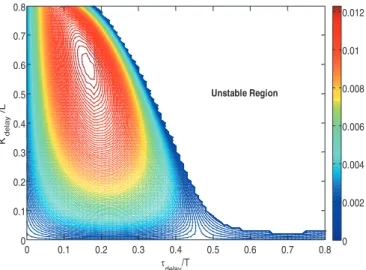
in order to enable us to obtain a map that represents the relation-ship between the damping of the load swing and the parameters of the anti-swing controller. To get this map, we assumed that the load swing was 20 degrees for the load swing angles and the remaining states for the helicopter and the load were zeros. We used the reciprocal of the swing index IHS as an indication of the level of damping as shown in Fig. 4. This map also shows the ranges of the control parameters that stabilized the system.
0 0.002 0.004 0.006 0.008 0.01 0.012
IJdelay/T
0 0.1 0.2 0.3 0.4 0.5 0.6 0.7 0.8
K
del
a
y
/L
0 0.1 0.2 0.3 0.4 0.5 0.6 0.7 0.8
Unstable Region
Figure 4. Damping map of the load swing (1/ISH) using DASC.
The highest damping level can be achieved at the follow-ing values (Eq. 31):
. , .
kd=kdx=kdy=0 67Lx=xdx=xdy=0 19TL (31)
where, TL=2r g Lis the period of oscillation of the
suspended load.
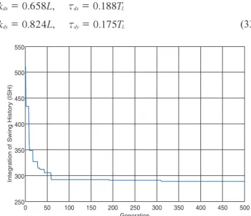
To get the optimal values of the four parameters that minimize the swing index ISH, we used the method of particle swarms. The following values were used for the PSO code (Eq. 32):
, ,
The evolution of the swing index (1/ISH) at each iteration
is showed in Fig. 5. The optimal parameters obtained using this technique were as in Eq. 33:
(33)
250 300 350 400 450 500 550
In
te
g
ra
ti
o
n
o
f
S
wi
n
g
H
isto
ry
(
IS
H)
Generation
0 50 100 150 200 250 300 350 400 450 500
Figure 5. Evolution of the PSO code.
The minimum value for ISH corresponding to these
param-eters was found to be 288, while it was 294 when we assumed the same gains for the longitudinal and lateral motions. This result is expected since we have more freedom than the case when we have only two parameters.
The time history of the helicopter CG, suspended load swing angles, and the Euler angles are shown in Figs. 6 to 9, using the optimal gains obtained from PSO. These
¿JXUHV VKRZ WKH HIIHFWLYHQHVV RI WKH SURSRVHG FRQWUROOHU
in suppressing the load swing. The anti-swing controller perturbs the helicopter form its initial position, but it returns it back due to the stability of the whole system. The maxi-mum deviation in helicopter position is nearly 5 ft, which can be considered small. However, this value can be more decreased by choosing small values of the anti-swing gain (k
dZLWKRXWVLJQL¿FDQWGHFUHDVHLQWKHOHYHORIVZLQJGDPS
-ing. The damping map can help in choosing the value of such gain. As shown in the map, with K = 0.3 and IJ = 0.2, we
can get high level of damping, which is comparable to that one obtained using the optimal gains but with small value for the traveling distance of the helicopter. The value of ISH
recorded in this case is 420.
-6 -5 -4 -3 -2 -1 0 1 2 3
Helicopter
Position
(ft)
0 20 40 60 80 100
Sec
z y x
Figure 6. Time history of the helicopter CG using DASC with the
optimal gains.
-20 -15 -10 -5 15 20 25
10
Load Swing Angles (deg)
0 5
0 20 40 60 80 100
Sec
L
L
I
ș
Figure 7. Time history of the load swing angles using DASC with
optimal gains.
-3 -2.5 -2 -1.5 -1 -0.5 0 0.5 1 1.5 2
Helicopter
Position
(ft)
Sec
0 20 40 60 80 100
x
y
z
Figure 8. Time history of the helicopter CG using DASC with
K
0 20 40 60 80 100 Sec
-25 -20 -15 -10 -5 10 15 20 25
Load Swing Angles (deg)
0 5
L
L
I
ș
Figure 9. Time history of the load swing angles using DASC with
Kd DQGIJd 7L.
Robustness
It can be shown by simulation that the designed system is robust with the changes of the load mass as indicated in Table 1. Moreover, the control parameters of the controller are functions of the load cable length. This robustness is due to the integration of the tracking controller, which is based on LQR technique and the time-delayed anti-swing controller.
Table 1. Performance of DASC with variation of load weight.
mr 0.3 0.5 0.7 0.9
ISH 339 288 251 221
Table 2. Performance of DASC with variation of the suspension
point location.
Location
xh yh zh
xh yh zh
xh yh zh
xh yh zh
ISH 267 272 320 316
CONCLUSIONS
A new anti-swing controller for helicopter slung load V\VWHPQHDUKRYHUÀLJKWZDVSURSRVHG7KLVFRQWUROOHUZDV based on time-delayed feedback of the load swing angles. The output from this controller was an additional displacement, which was added to the helicopter trajectory in the longitudinal and lateral directions. Hence, its implementation is simple and LWRQO\QHHGVDVPDOOPRGL¿FDWLRQWRWKHVRIWZDUHRIKHOLFRSWHU position controller.
To implement the proposed anti-swing controllers, a tracking controller for the helicopter was designed using the LQR technique. The function of the tracking controller is to stabilize the helicopter and track the trajectory generated by the anti-swing controller.
A map that represents the level of damping achieved by the proposed anti-swing controller was constructed as function of the controller parameters. To consider the coupling between the in-plane and out-of-plane load swings, the PSO algorithm was used to get the optimal gains for controlling the swing of both motions. The simulation results show the effectiveness of proposed controller in suppressing the load swing. For initial disturbance of the load swing angles, the anti-swing controller makes the helicopter slightly moves from its rest position to damp the swing motion, then it returns the helicopter back to its nominal position due to the stability of the whole system and the damping added to the load swing by the time-delayed anti-swing controller. The parameters of the controller can be chosen to keep the helicopter deviated from hovering position within acceptable limits.
ACKNOWLEDGMENTS
The author acknowledges the support of King Fahd Univer-sity of Petroleum and Minerals, under Grant SB080024.
REFERENCES
Abzug, M., 1970, “Dynamics and control of helicopters with two cable sling loads”, In AIAA 2nd Aircraft Design and Operations Meeting, number AIAA-70-929, American Institute of Aeronautics and Astronautics.
Asseo, S. and Whitbeck, R., 1973, “Control requirements for sling-load stabilization in heavy lift helicopters”, Journal of the American Helicopter Society, Vol. 18, pp. 23-31.
Bisgaard, M. et al., 2006, “Modeling of a Generic Slung Load System”, In AIAA Modeling and Simulation Conference, Colorado.
Cera, J. and Farmer, S.W. J., 1974, “A Method of Automatically Stabilizing Helicopter Sling Loads”, Technical Note NASA-TN-D-7593, NASA Langley Research Center.
Cicolani, L. and Kanning, G., 1992, “Equations of Motion of Slung-load Systems”, Including Multilift Systems, Technical Paper NASA-TP-3280, NASA Ames Research Center.
Fusato, D. et al., 1999, “Flight Dynamics Of An Articulated
Rotor Helicopter with an External Slung Load”, American Helicopter Society 55th Annual Forum, Montreal, Canada.
Kennedy, J., 1997, “The Particle Swarm: Social Adaptation of Knowledge”, In Proceedings of the 1997 IEEE international Conference on Evolutionary Computation ICEC’97, Indianapolis, Indiana, USA, pp. 303-308.
Masoud, Z.N. et al., 2002, “Sway reduction on container
cranes using delayed feedback controller”, In Proceedings of the 43rd AIAA/ASME/ASCE/AHS/ASC Structures, Structural Dynamics, and Materials Conference, Denver, CO, AIAA-2002-1279.
Omar H. M. and Nayfeh, A.H., 2005, “Anti-swing control of gantry and tower cranes using fuzzy and time-delayed feedback with friction compensation” , Shock And Vibration, Vol. 12, No. 2, pp. 73-89.
Omar, H.M., 2005, “Dynamics of helicopter slung load system near hover” Technical Report, Aerospace Department, KFUPM.
Poli, C. and Cromack, D., 1973, “Dynamics of Slung Bodies Using a Single-Point Suspension System”, Journal of Aircraft, Vol. 10, No. 2, pp. 80-86.
Prouty, R.W., 2003, “Helicopter Performance, Stability, and Control”, Kreiger Publishing Company.
Raz, R. et al., 1989, “Active aerodynamic stabilization of a
helicopter/sling-load system”, AIAA Journal of Aircraft, Vol. 26, pp. 822-828.
Shi, Y. and Eberhart, R., 1998, “Parameter Selection in Particle Swarm Optimization”, In Proceedings of the 7th Annual Conference on Evolutionary Programming, pp. 591-600.
Stuckey, R.A., 2001, “Mathematical Modeling of Helicopter Slung-Load Systems”, Technical Report, Air Operations Division, Aeronautical and Maritime Research Laboratory, Australia.