www.scielo.br/cam
An interior point method for constrained
saddle point problems
ALFREDO N. IUSEM1∗ and MARKKU KALLIO2 1Instituto de Matemática Pura e Aplicada, Estrada Dona Castorina, 110
22460, Rio de Janeiro, RJ, Brazil
2Helsinki School of Economics, Runeberginkatu 14-16, 00100 Helsinki, Finland E-mail: [email protected] / [email protected]
Abstract. We present an algorithm for the constrained saddle point problem with a convex-concave functionLand convex sets with nonempty interior. The method consists of moving away from the current iterate by choosing certain perturbed vectors. The values of gradients ofL
at these vectors provide an appropriate direction. Bregman functions allow us to define a curve which starts at the current iterate with this direction, and is fully contained in the interior of the feasible set. The next iterate is obtained by moving along such a curve with a certain step size. We establish convergence to a solution with minimal conditions upon the functionL, weaker than Lipschitz continuity of the gradient ofL, for instance, and including cases where the solution needs not be unique. We also consider the case in which the perturbed vectors are on certain specific curves starting at the current iterate, in which case another convergence proof is provided. In the case of linear programming, we obtain a family of interior point methods where all the iterates and perturbed vectors are computed with very simple formulae, without factorization of matrices or solution of linear systems, which makes the method attractive for very large and sparse matrices. The method may be of interest for massively parallel computing. Numerical examples for the linear programming case are given.
Mathematical subject classification:90C25, 90C30.
Key words: saddle point problems, variational inequalities, linear programming, interior point methods, Bregman distances.
#581/03. Received: 13/V/03. Accepted: 09/I/04.
1 Introduction
In this paper, we discuss methods for solving constrained saddle point problems. Given closed convex setsX,Y contained inRn,Rmrespectively, and a function L : X ×Y → R, convex in the first variable and concave in the second one, the saddle point problem SPP(L,X,Y) consists of finding(x∗, y∗)∈X×Y such that
L(x∗, y)≤L(x∗, y∗)≤L(x, y∗) (1)
for all (x, y) ∈ X ×Y. SPP(L,X,Y) is a particular case of the variational inequality problem, which we describe next. Given a closed convex setC ⊂Rp
and a maximal monotone operatorT : Rp → P(Rp), VIP(T,C) consists of
findingz∈Csuch that there existsu∈T (z)satisfying
ut(z′−z)≥0 (2)
for allz′ ∈C. If∂xL,∂yLdenote the subdifferential and superdifferential ofL
in each variable (i.e. the sets of subgradients and supergradients) respectively, and we defineT :Rn×
Rm→P(Rn×
Rm)asT =(∂xL,−∂yL)then VIP(T,C)
coincides with SPP(X,Y) if we takep =m+nandC =X×Y. It is easy to check that thisT is maximal monotone.
It is well known that whenT =∂f for a convex functionf (x)then VIP(T,C) reduces to minf (x)s.t. x ∈ C. This suggests the extension of optimization methods to variational inequalities. In the unconstrained caseC =Rn, for which
VIP(T,C) consists just of finding a zero ofT, i.e. az∗such that 0∈T (z∗), one could attempt the natural extension of the steepest descent method, i.e.
zk+1=zk−αuk
withuk ∈T (zk)andα >0. This simple approach works only under very restric-tive assumptions onT (strong monotonicity and Lipschitz continuity, see [1]). An alternative one, which works under weaker assumptions, is the following: move in a direction contained in −T (zk) finding an auxiliary (or perturbed)
pointwkand then move fromzkin a direction contained in−T (wk), i.e.
wk =zk−αkuk (3)
withuk ∈T (zk),dk ∈T (wk), andαk,α¯k >0. In the constrained case, one must
project ontoC in order to preserve feasibility, i.e., one takes
wk =PC(zk−αkuk) (5)
zk+1=PC(zk− ¯αkdk) (6)
wherePCis the orthogonal projection ontoC. IfT is Lipschitz continuous with
constantπ, then convergence of{zk}to a solution of VIP(T,C) is guaranteed by
takingαk = ¯αk = α ∈ (0,1/π ). This result can be found in [16], where the
method was first introduced. In the absence of Lipschitz continuity (or when the Lipschitz constant exists but is not known beforehand) it has been proven in [11] that the algorithm still converges to a solution of VIP(T,C) ifαk,α¯kare
determined through a certain finite bracketing procedure. A somewhat similar method has been studied in [15].
WhenChas nonempty interior, it is interesting to consider interior point meth-ods, i.e. such that{wk}and{zk}are contained in the interiorCoofC, thus doing
away with the projectionPC. This can be achieved if a Bregman functiongwith
zoneCois available. Loosely speaking, such ag is a strictly convex function which is continuous inC, differentiable inCoand such that its gradient diverges at the boundary ofC. Withgwe construct a distanceDgonC×Coas
Dg(w, z)=g(w)−g(z)− ∇g(z)t(w−z) (7)
and instead of the half line{z−t u:t ∈R+}we consider the curve{sg(z, u, t ): t ∈ R+}wheresg(z, u, t )is the solution of minw∈C{utw+(1/t )Dg(w, z)}for t >0, or equivalentlysg(z, u, t )is the solutionwof
∇g(w)= ∇g(z)−t u, (8)
which allows us to extend the curve tot=0. Under suitable assumptions ong (see Section 2),sg(z, u,0)=z, the curve is uniquely defined fort ∈ [0,∞)and
it is fully contained inCo. The idea is to replace (5) and (6) by
wk =sg(zk, uk, αk) (9)
withuk,dk,αkandα¯kas in (3) and (4). This algorithm was proposed in [3], where
it is proved that convergence of{zk}to a solution of VIP(T,C) is guaranteed if αkis chosen through a given finite bracketing procedure andα¯k solves a certain
nonlinear equation in one variable. A slight improvement is presented in [12], where it is shown that convergence is preserved whenα¯k is also found through
another finite bracketing search. The main advantage of these interior point methods with Bregman functions as compared e.g. to Korpelevich’s algorithm lies in the fact that no orthogonal projections onto the feasible set are needed, since all iterates belong automatically to the interior of this set. A detailed discussion of the computational effects of this advantage in the case in whichC is an arbitrary polyhedron with nonempty interior can be found in Section 6 of [3]. For SPP(L,X,Y), when eitherXorY is an arbitrary polyhedron with nonempty interior, the method introduced in this paper presents the same advantage over the algorithm in [13], discussed in the next paragraph, which requires orthogonal projections ontoXandY.
Going back to SPP(L,X,Y), another related method is presented in [13]. Given a point(xk, yk), a rather general perturbed vector wk = (ξk, ηk)is computed, and then
xk+1=PX(xk − ¯αkdxk) (11) yk+1=PY(yk + ¯αkdyk) (12)
withdk
x ∈∂xL(xk, ηk)anddyk ∈∂yL(ξk, yk). In this case no search is required
for the step sizeα¯k, which is given by a simple formula in terms of the gap L(xk, ηk)−L(ξk, yk). The difficulty is to some extent transferred to the selection
of(ξk, ηk), which must satisfy certain conditions in order to ensure convergence to a solution of SPP(L,X,Y). One possibility is to adopt (5) so thatξk =PX(xk− αkukx), η
k = P
Y(yk +αkuky), with u k
x ∈ ∂xL(xk, yk), uky ∈ ∂yL(xk, yk). In
this case the method is somewhat similar to Korpelevich’s (see [16]), but not identical: in linear programming, for instance, a closed expression forαk is
easily available for the method of [13] even when a Lipschitz constant for∇Lis not known beforehand. Other differences between the method in [13] with this choice of(ξk, ηk)and Korpelevich’s are commented upon right after Example 6 in Section 3.
(ξk, ηk). Taking advantage of this fact, we will combine the approaches in [3] and [13], producing an interior point method for the case of nonemptyXo×Yo.
We will consider two independent modifications upon the method in [13]. The first one to be discussed in Section 3 is the following: assuming that Bregman functionsgX,gY with zonesXo,Yorespectively are available, we will use (10)
instead of (11) and (12), setting
xk+1=sgX(x
k
, dxk, τk) (13)
yk+1=sgY(y
k,−dk
y, τk). (14)
We will show that if the perturbation pair(ξk, ηk)satisfies conditions required
in [13] and the stepsizesτk are chosen in a suitable way then convergence to a
solution follows.
It is clear that the algorithm becomes practical only whensgX,sgY have explicit
formulae, i.e., in view of (8), when∇gX,∇gY are easily invertible. Bregman
functions with this property are available for the cases in whichC is an orthant, a box, or certain polyhedra (in the latter case, inversion of the gradient requires solution of two linear systems) and are presented in [3]. Examples of realizations of this method are given are Section 4.
The second modification presented in Section 5 consists of an interior point procedure for the determination of(ξk, ηk), namely
ξk =argmin
u∈X
{L(u, yk)+(1/λ)DgX(u, x
k)} (15)
ηk =argmax
v∈Y
{L(xk, v)−(1/µ)DgY(v, y
k)} (16)
whereλ,µare positive constants. Definitions (15) and (16) imply
ξk =sgX(x
k
,d˜xk, λ) (17)
ηk =sgY(y
k,− ˜dk
y, µ) (18)
withd˜k
x ∈ ∂xL(ξk, yk),d˜yk ∈ ∂yL(xk, ηk). Equivalently with (17) and (18) we
have
Differently from (13) and (14), equations (17) and (18) are implicit inξk, ηk, which appear in both sides of (19) and (20). These equations cannot be in general explicitly solved, even when∇gX,∇gY are easily invertible. On the other hand,
no search is needed for perturbation stepsizes λand µ even when ∇L is not Lipschitz continuous. This choice of(ξk, ηk)does not satisfy the conditions in [13], so that the general convergence result for the sequence defined by (13) and (14) cannot be fully used. A special convergence proof will be given assuming that the Bregman functions are separable and the constraint setsXandY are the nonnegative orthants.
It is immediate that (19) and (20) become explicit equations (up to the inversion of∇gX and∇gY) when∂xL(·, y),∂yL(x,·)are constant. This happens in the
case of linear programming. For this case, combining both modifications, we obtain an interior point method with explicit updating formulae both for the perturbed points and the primal and dual iterates. The curvilinear stepsizeτk
requires a simple search. We analyze the linear programming case in detail in Section 6, where we present also some numerical illustration of the method.
2 Bregman functions and distances
LetC ⊂Rpbe a closed and convex set and letCobe the interior ofC. Consider g:C→Rdifferentiable inCo. Forw∈Candz∈Co, defineDg:C×Co→R
by (7).Dgis said to be the Bregman distance associated tog.
We say thatgis aBregman function with zoneC if the following conditions hold:
B1. gis continuous and strictly convex onC.
B2. g is twice differentiable on Co, and in any bounded subset of Co the
eigenvalues of∇2g(z)are bounded below by a strictly positive number. B3. The level sets of Dg(w,·) andDg(·, z)are bounded, for all w ∈ C,
z∈Co, respectively.
B4. If{zk} ⊂Coconverges toz∗, then limk→∞ Dg(z∗, zk)=0.
The definition of Bregman functions and distances originates in [2]. They have been widely used in convex optimization, e.g. [4], [5], [6], [7], [8]. Condition B2 in these references is weaker than here; only differentiability ofginCois
required. On the other hand, such references included an additional condition which is now implied by our stronger condition B2, namely the result of Propo-sition 1 below. Condition B5 is calledzone coercivenessin [3]. From (7) and B1 it is immediate that for allw ∈C,z∈Co,Dg(w, z)≥0 andDg(w, z) =0
if and only ifw=z.
We present next some examples of Bregman functions.
Example 1. C =Rp,g(x)= x2. ThenD
g(w, z)= w−z2.
Example 2. C = Rp+, g(z) =
p
j=1zjlogzj, continuously extended to the
boundary ofC with the convention that 0 log 0=0. Then
Dg(w, z)= p
j=1
[wjlog(wj/zj)+zj −wj]. (21)
Dgis the Kullback-Leibler information divergence, widely used in statistics.
Example 3. C =Rp+,g(z)=p
j=1(z
α j −z
β
j), withα >1,β ∈(0,1).
Examples of Bregman functions satisfying these conditions for the cases ofC being a box or a polyhedron can be found in [3]. We now proceed to a result which will be employed in the convergence analysis.
Proposition 1. Ifgis a Bregman function with domainCo, and{zk}and{wk} are sequences inCosuch that{zk}is bounded andlimk→∞Dg(wk, zk)=0, then
lim
k→∞z k−
wk =0.
Proof. LetB ⊂ Rn be a closed ball containing{zk} such that, for anyz on the boundary of B, zk −z > 1, for allk. Forν ∈ [0,1] define zk(ν) = νwk +(1−ν)zk. Let ν
eachk, define uk = zk(νk). Since Co is convex and ν ∈ [0,1], we get that zk(ν
k)∈Co. By convexity ofDg(·, zk),
0≤Dg(uk, zk)≤Dg(wk, zk).
BecauseDg(wk, zk)converges to zero, so doesDg(uk, zk). We shall show that
zk −uk converges to zero. Then, from the definition of B it follows that there existsk′such that, for allk > k′,ukis in the interior ofB, such thatνk =1
anduk =wk; hence the assertion follows.
Defineuk(ω)=ωuk +(1−ω)zk, forω∈ [0,1]. By Taylor’s Theorem,
g(uk) = g(zk)+ ∇g(zk)t(uk−zk)
+ 1 2(u
k −zk)t
∇2g(uk(ω))
(uk−zk) (22)
for someω ∈ [0,1]. The quadratic term in (22) is equal toDg(uk, zk), which
converges to zero. Because of boundedness of{zk}and{uk}, B2 implies that Dg(uk, zk)is bounded below byθuk−zk2for someθ >0 and independent
ofk. Thereforeuk−zkconverges to zero.
3 An interior point method for saddle point computation
In this section we assume thatXandY have nonempty interior and thatgXand gY are Bregman functions with zonesXandY, respectively. L:Rn×Rm→R
is continuous onX×Y, convex in the first variable and concave in the second one.
Following [13] we introduce perturbation sets:X×Y →P(X),Ŵ:X× Y →P(Y ). We consider the following properties of,Ŵ.
A1. If (x, y) ∈ Xo ×Yo and (ξ, η) ∈ (x, y)×Ŵ(x, y) then L(x, η)− L(ξ, y)≥0, with strict inequality if(x, y)is not a saddle point.
A2. IfE⊂Xo×Yois bounded then∪
(x,y)∈E(x, y)and∪(x,y)∈EŴ(x, y)are
bounded.
A3. If{(uℓ, vℓ)} ⊂X×Y converges to(u, v)asℓgoes to∞,ξℓ ∈(uℓ, vℓ), ηℓ ∈Ŵ(uℓ, vℓ)and limℓ→∞[L(uℓ, ηℓ)−L(ξℓ, vℓ)] =0 then(u, v)solves
We give next a few examples of sets,Ŵ, taken from [13].
Example 4. Assume that X and Y are compact and define (x, y) = argminξ∈XL(ξ, y)andŴ(x, y)=argmaxη∈YL(x, η).
Example 5. Letλ >0,µ >0 and define(x, y)=argminξ ∈X[L(ξ, y)+ λξ −x2] and Ŵ(x, y) = argmax
η∈Y[L(x, η)−µη−y2], for x ∈ X, y∈Y. Due to strict convexity (concavity) of the minimand (maximand),(x, y) (Ŵ(x, y)) is uniquely determined.
Example 6. Assume that ∇xL and ∇yL are Lipschitz continuous with
con-stant π and let 0 < α < 1/π. Define (x, y) = {PX(x −α∇xL(x, y))}
andŴ(x, y) = {PY(y +α∇yL(x, y))}. It corresponds to the perturbed vector wk of Korpelevich’s method ([16]) in (5). But we must point out that when
we use the method in [13] (i.e. (11)-(12)) with this perturbation we obtain something quite different from Korpelevich’s method, because Korpelevich’s method, withT = (∇xL,−∇yL), would then choose dxk = ∇xL(ξk, ηk) and dyk = ∇yL(ξk, ηk), while the method in [13] takes dxk = ∇xL(xk, ηk) and dk
y = ∇yL(ξk, yk). This choice of dxk, dyk is possible only in the case of a
saddle point problem, where we have two variablesxandy, while Korpelevich’s method is devised for a general variational inequality problem, where we only have the vectorwk, instead of the pair(ξk, ηk).
It is not difficult to prove that the choices ofandŴmade in Examples 4-6 satisfy conditions A1-A3.
Next we present the algorithm generating the sequence{(xk, yk)}. We denote zk =(xk, yk),C =X×Y andCo =Xo×Yo, and defineD
g :C ×Co→R
employing
g(z)=gX(x)+gY(y). (23)
It is a matter of routine to check thatgis a Bregman function with zoneC. The algorithm of this section is defined as follows:
Step 0: Initialization. Choose parametersβandγ, 1> β≥γ >0, and take
Step 1: Perturbation. Begin iteration withzk =(xk, yk). Choose perturba-tion vectors(ξk, ηk)∈(xk, yk)×Ŵ(xk, yk)and define
σk =L(xk, ηk)−L(ξk, yk). (25)
Step 2: Stopping test. Ifσk =0 then stop.
Step 3: Direction. Choose dxk ∈ ∂xL(xk, ηk), and dyk ∈ ∂yL(ξk, yk), and
denotedk =(dk
x,−dyk)t.
Step 4: Stepsize. Fort ≥0 define functions
z(t )=sg(zk, dk, t ) (26)
and
φk(t )=t σk−Dg(zk, z(t )). (27)
Search for a step sizeτk ≥0 satisfying
γ σkτk ≤φk(τk)≤βσkτk. (28)
Step 5: Update. Set
zk+1=z(τk), (29)
incrementkby one and return to Step 1.
Theorem 1 below shows thatφk(t )is a concave function withφk(0)=0 and φk′(0)=σk >0. For iterationkand a potential stepsizet, this function provides
Theorem 1. Assume that SPP(L,X,Y) has solutions. Let g be a Bregman function with zoneCoand let{zk}be a sequence generated by the algorithm of this section, whereξk ∈ (zk) andηk ∈ Ŵ(zk), with andŴ satisfyingA1 andA2. If the algorithm stops at iterationk, thenzk solves SPP(L,X,Y). If the sequence{zk}is infinite, then
i) zkis well defined and belongs toCo, for allk,
ii) for any solution z∗ of SPP(L,X,Y), the Bregman distanceDg(z∗, zk)is monotonically decreasing,
iii) {zk}is bounded,
iv) limk→∞σk =0;
v) limk→∞zk+1−zk =0;
vi) if additionally A3 is satisfied, then the sequence {zk} converges to a solution of SPP(L,X,Y).
Proof. We prove first (i) by induction. z0belongs toCo by (24). Assuming thatzkbelongs toCo, note that (26) is equivalent to
∇g(z(t ))= ∇g(zk)−t dk, (30)
so that by B1 and B5,z(t )is uniquely defined by (30) and belongs toCofor all t ≥0. By (29),zk+1belongs toCoand (i) holds. Now we consider the case of finite termination, i.e. when, according to Step 2,σk =0. In such a case, since zk belongs toCoby (i), it follows from A1 thatzk is a saddle point. From now
on we assume that{zk}is infinite. We proceed to prove (ii). Sincez(t )∈Cofor
allt ≥0, using (7) and (30) we get
Dg(z∗, zk)−Dg(z∗, z(t ))= −t (dk)t(z∗−zk)−Dg(zk, z(t )). (31)
By convexity/concavity ofL, since(x∗, y∗)is a saddle point,
−(dk)t(z∗−zk) ≥ −L(x∗, ηk)+L(xk, ηk)+L(ξk, y∗)−L(ξk, yk) = σk−L(x∗, ηk)+L(ξk, y∗)≥σk
Combining (27), (31) and (32) yields
Dg(z∗, zk)−Dg(z∗, z(t ))≥φk(t ). (33)
Differentiating (30) yields
∇2g(z(t ))d
dtz(t )= −d k
so that the first two derivatives ofφk(t )in (27) are
φk′(t )=σk+(dk)t(z(t )−zk) (34)
and
φk′′(t )= −ϕk(t ), (35)
withϕk defined as
ϕk(t )=(dk)t[∇2g(z(t ))]−1dk. (36)
Since z(0) = zk, φ
k(0) = 0. By A1 and (34), φk′(0) = σk > 0, in view of
the stopping criterion, and so (32) impliesdk = 0. Consequently by B2, (35)
and (36), φk′′(t ) < 0. Therefore φk(t ) is a concave function of t ∈ [0,∞)
with a positive slope att = 0. Inequality (33) implies that φk(t )is bounded
above. Hence there exists a stepsize τk satisfying (28), so that zk+1 is well
defined, and therefore item (i) follows from (30). Furthermore, for someγk ∈
[γ , β], φk(τk) =γkτkσk which together with (33) implies item (ii). Denote by Bothe set{z∈ Co:D
g(z∗, z)≤ Dg(z∗, z0)}. By B3,Bois bounded. Item (ii)
implies thatzk+1∈Boifzk ∈Bo. Therefore, item (iii) follows then by induction
from (24).
Since{zk}is bounded, we get from A2 that{(ξk, ηk)}is bounded. The oper-ator(∂xL,−∂yL)is maximal monotone, therefore bounded over bounded sets
contained in the interior of its domain, which in this case isRn×Rm(e.g. [18]).
It follows that{dk}is bounded.
By Taylor’s theorem and (28), for someτˆ ∈ [0, τk], φk(τk)=τkσk− τk2
2ϕk(τ )ˆ ≤
βτkσk.Consequently, and because B2, A2 and item (iii) imply ϕk(τ )ˆ ≤ θ, for
someθ >0, we have
τk ≥
2(1−β)σk ϕk(τ )ˆ
≥ 2(1−β)σk
By (28) and (33),
k
τkσk <∞. (38)
By (38), limk→∞τkσk =0, and then, multiplying both sides of (37) byσk, we
conclude that limk→∞σk = 0, i.e. (iv) holds. From (27) and (28) we have
0 ≤ Dg(zk, zk+1) ≤ τkσk, where the right side converges to zero. Therefore,
item (v) follows from item (iii) and Proposition 1. By item (iii) the sequence {zk}has an accumulation pointz¯. By item (iv) and A3, z¯ solves SPP(L,X,Y). By item (ii) the Bregman distance Dg(z, z¯ k) is non-increasing. If {zjk} is a
subsequence of{zk}which converges toz¯, by B4 lim
k→∞Dg(z, z¯ jk)=0. Since
{Dg(z, z¯ k)}is a nondecreasing and nonnegative sequence with a subsequence
which converges to 0, we conclude that the whole sequence converges to 0. Now we apply Proposition 1 withwk = ¯z, and conclude that limk→∞zk = ¯z.
4 Particular realizations of the algorithm
In the unrestricted case (X =Rn,Y =Rm) we can takegas in Example 1 so that
z(t )=zk− t 2d
k and
φk(t )=t σk− t2
4d
k2
.
In this case, withβ=γ =0.5, we may chooseτkto maximizeφk(t )yielding
τk =
2σk
dk2 and z
k+1=zk− σk
dk2d
k,
which is a special case of the method considered in [13].
Next, consider the case in whichX,Y are the nonnegative orthants. Forgas in Example 2 we have
∇g(z)j =1+logzj (39)
∇2g(z)−1=diag(z
1, . . . , zn) (40)
z(t )j =zjkexp(−t d k
j) (41)
φk(t )=t σk −
j zkj
t djk−1+exp(−t d k j)
(42)
In this case, a search is needed for determining the stepsize τk in Step 3 of
5 An interior point procedure for perturbation
In this section we analyze a selection rule for specifyingξkandηkwhich extends
the proposal of Example 6 in Section 3. LetgXandgYbe Bregman functions with
zonesXoandYo, respectively. Takeλ >0 andµ >0, and for(x, y)∈Xo×Yo
define
ξ =ξ(x, y)=argmin
u∈X
L(u, y)+1
λDgX(u, x)
(43)
η=η(x, y)=argmax
v∈Y
L(x, v)− 1
µDgY(v, y)
. (44)
We shall restrict the discussion to the following special case of SPP(L,X,Y): X = Rn
+, Y = Rm+, L twice continuously differentiable on Rn ×Rm andg
separable, i.e.
gX(x)= n
j=1 ˜
gj(xj), gY(y)= m
i=1 ˆ gi(yi).
We will show that the perturbation sets defined by (43)-(44) satisfy A1 and A2. A3 does not hold in general for this perturbation, but we will establish convergence of the method under a nondegeneracy assumption on the problem, and, in the case of linear programming, without such assumption. Our proof can be extended to nondifferentiableLand to box, rather than positivity, constraints, at the cost of some minor technical complications.
Proposition 2. Assume thatLis continuously differentiable,X×Y =Rn +×Rn+, and that g is a separable Bregman functions with zone Xo ×Yo. Consider (x, y)∈Xo×Yoand(ξ, η)as in (43)-(44). Then
i) (ξ, η)is uniquely determined and(ξ, η)∈Xo×Yo;
ii) if(x, y)is not a saddle point, thenL(x, η)−L(ξ, y) >0;
Proof. Letf (u)=L(u, y)+1/λDgX(u, x). Takew= ∇xL(x, y)and define
¯
f (u)=L(x, y)+wt(u−x)+1/λD
gX(u, x). By convexity ofL(·, y)we have
¯
f (u)≤f (u) (45)
for allu∈X. Consider the unrestricted minimization problem minf (u)¯ , whose optimality conditions are∇gX(u) = ∇g(x)−λw. By B5, this equation inu
has a unique solutionu¯ which belongs to Xo. It follows easily from (7) that DgX(·, x)is strictly convex, and the same holds forf¯, so thatu¯ minimizesf¯in
Rn. A strictly convex function which attains its minimum has bounded level sets,
and it follows from (45) thatf also has bounded level sets (see [19, Corollary 8.7.1]), and therefore it attains its minimum inX. Being the sum of a convex function and a strictly convex one,f is strictly convex and so the minimizer is unique, by convexity ofX. The fact that this minimizer belongs toXo follows
from B5 and has been established in [10, Theorem 4.1]. By definition of f, this minimizer isξ(x, y). A similar proof holds forη(x, y)so that the proof of item (i) is complete.
For item (ii), assume that(x, y)is not a saddle point. Then∇xL(x, y) = 0
or∇yL(x, y) = 0. Assume that the former case holds; the latter one can be
analyzed similarly. Observe that
∇f (u)= ∇xL(u, y)+
1
λ[∇gX(u)− ∇gX(x)] (46) so that∇f (x)= ∇xL(x, y)= 0. Hencex is not a solution of (43) and
conse-quently
f (x)=L(x, y) > L(ξ, y)+1
λDgX(ξ, x) > L(ξ, y).
This implies L(x, y)−L(ξ, y) > 0. Similarly, L(x, η)−L(x, y) ≥ 0 and thereforeL(x, η)−L(ξ, y) >0. This completes the proof of item (ii).
To prove item (iii), we will prove boundedness of{ξ(x, y) :(x, y) ∈ B}. A similar argument holds forη(x, y). The proof relies on successive relaxations for optimization problems, whose optimal objective function values are upper bounds forξ2. Since∇f (ξ )=0 by (46),ξis unique by item (i), and we have
ξ2=max{u2|u≥0,∇g
Note that
{u≥0| ∇gX(u)− ∇gX(x)= −λ∇xL(u, y)}
⊂
u≥0|ut∇gX(u)− ∇gX(x) = −λut∇xL(u, y)
⊂
u≥0|ut
∇gX(u)− ∇gX(x) ≤ −λut∇xL(u, y)
⊂
u≥0|gX(u)−gX(0)≤ut
∇gX(x)−λ∇xL(0, y) ,
(47)
using the facts that ut∇xL(u, y)− ∇xL(0, y) ≥ 0 and gX(u) −gX(0) ≤ ut∇gX(u), which result from convexity ofgXandL(·, y), in the last inclusion
of (47).
Let nowρ=maxj{sup(x,y)∈B[ ˜gj′(xj)−λ∇xL(0, y)j]}. We claim thatρ <∞.
It suffices to show that sup(x,y)∈B[ ˜gj′(xj)−λ∇xL(0, y)j]<∞for allj, which
follows from the facts that∇xL(0, y) is continuous as a function ofy, g˜′j is
continuous inR++, limt→0g˜j′(t )= −∞, because of B5, andBis bounded. The
claim is established. It follows from (47) that
{u≥0| ∇gX(u)− ∇gX(x)= −λ∇xL(u, y)}
⊂ {u≥0|gX(u)−gX(0)≤ρstu} = {u≥0| gX(u)−ρstu≤gX(0)}.
wherest =(1,1, . . . ,1). We claim that the set{u≥0|g
X(u)−ρstu≤gX(0)}
is bounded. Note that this set is a level set of the convex functiong¯X(u) = gX(u)−ρstuand that∇ ¯gX(u)= ∇gX(u)−ρs. By B5, there existsz >0 such
that∇gX(z)=ρs, i.e.∇ ¯gX(z)=0, so thatzis an unrestricted minimizer ofg¯X.
Since∇2g¯
X = ∇2gX, we get from B2 that ∇2g¯X(u)is positive definite for all u >0, and henceg¯Xis strictly convex andzis its unique minimizer. Thus, the
level set ofg¯X corresponding to the valueg¯X(z)is the singleton{z}. It is well
known that if a convex function has a bounded level set, then all its nonempty level sets are bounded, which establishes the claim. It follows that
ξ2 = max{u2|u≥0,∇gX(u)− ∇gX(x)= −λ∇xL(u, y)}
≤ max{u2| u≥0, gX(u)−ρstu≤gX(0)}<∞,
(48)
We use now (43) and (44) to define perturbation setsandŴconsisting of single elements ξ andη, respectively. In view of Proposition 2, this rule of perturbation satisfies conditions A1 and A2. However, the following example demonstrates that A3 may not hold.
Takem=n=1,λ =µ=1,gas in Example 2 andL(x, y) =(x−1)2− (y−1)2, whose only saddle point is(1,1). In this case the optimality conditions for (43)-(44) become
2(ξ−1)+logξ =logx (49)
2(η−1)+logη=logy. (50)
Take a sequence {(xk, yk)}convergent to(0,0). Then the right hand sides of
(49)-(50) diverge to−∞, implying that logξk and logηk also diverge to−∞;
i.e.{(ξk, ηk)}also converges to(0,0). It follows that
lim
k→∞[L(x k
, ηk)−L(ξk, yk)] =L(0,0)−L(0,0)=0,
but(0,0)is not a saddle point ofL.
This example shows that the convergence argument of Theorem 1 is no longer valid for our algorithm with perturbation sets chosen according to (43)-(44). Instead, we provide another convergence argument, which can be more easily formulated in terms of variational inequalities and nonlinear complementarity problems. We need two results on these problems. The first one is well known, while the second one is, to our knowledge, new, and of some interest on its own.
Proposition 3.
i) IfT :Rp→Rpis monotone and continuous, andC ⊂Rp is closed and convex, then the solution set of VIP(T,C), when nonempty, is closed and convex.
ii) IfC =Rp+then VIP(T,C) becomes the nonlinear complementarity prob-lem NCP(T), consisting of findingz∈Rpsuch that
T (z)j ≥0 (1≤j ≤p) (51)
zj ≥0 (1≤j ≤p) (52)
Proof. Elementary (see, e.g. [9]).
Corollary 1. IfX×Y =Rn
+×Rm+then(x,¯ y)¯ is a solution of SPP(L,X,Y) if and only if
¯
x∈X,y¯ ∈Y (54)
∇xL(x,¯ y)¯ j =0 for x¯j >0 (55)
∇xL(x,¯ y)¯ j ≥0 for x¯j =0 (56)
∇yL(x,¯ y)¯ i =0 for y¯i >0 (57)
∇yL(x,¯ y)¯ i ≤0 for y¯i =0 (58)
Proof.Follows from Proposition 3 withT =(∇xL,−∇yL).
Before presenting our new result, we need some notation.
Definition. We say that NCP(T) satisfies thestrict complementarity assump-tion(SCA from now on) if for all solutionszˆ of NCP(T) and for allj between 1 andpit holds that eitherzˆj >0 orT (z)ˆ j >0.
Forz ∈ Rp, letJ (z) = {j ∈ {1, . . . , p} : z
j =0}andI (z) = {1, . . . , p} \ J (z).
Proposition 4. Assume thatT is monotone and continuous and that NCP(T) satisfies SCA. Ifz¯ ∈ Rp satisfies (52) and (53), and J (z)¯ ⊂ J (z∗) for some solutionz∗of NCP(T), thenz¯solves NCP(T).
Proof. Letz(α)= ¯z+α(z∗− ¯z). We will prove thatz(α)satisfies (52)-(53) for allα ∈ [0,1], and also (51) for α close to 1; then we will show that if (51) is violated for someα ∈ [0,1] then SCA will be violated too. In order to prove thatz(α)satisfies (53) for allα ∈ [0,1]we must make a detour. Let U = {z ∈ Rp+ : zj = 0 for allj ∈ J (z)¯ }. A vectorzˆ solves VIP(T,U) if and
only ifzˆ ∈Uand
for allz∈U. Note thatz¯ ∈U. SinceJ (z)¯ ⊂J (z∗),z∗also belongs toU. We claim that bothz¯ andz∗ satisfy (59). This is immediate forz∗which satisfies (59) for allz ∈Rp+, since it solves NCP(T), equivalent, by Proposition 3(ii), to VIP(T,Rp+). Regardingz¯, we havez¯j =zj =0 for allz∈U and allj ∈J (z)¯ ,
so that terms withj ∈ J (z)¯ in the summation of (59) vanish. Forj /∈ J (z)¯ , we haveT (z)¯ j =0 becausez¯ satisfies (53), so that terms withj /∈ J (z)¯ in the
summation of (59) also vanish. Therefore bothz¯andz∗solve VIP(T,U), and so z(α)solves VIP(T,U) for allα ∈ [0,1]by Proposition 3(i). In particularz(α) satisfies (52) for allα ∈ [0,1]. We look now at (53). Sincez(α)∈U, we have z(α)j = 0 for j ∈ J (z)¯ , i.e. (53) holds for suchj’s. Ifj ∈ I (z)¯ , we takez1
andz2defined asz1ℓ = z2ℓ = 0 for ℓ = j, z1j = 2z(α)j, zj2 = (1/2)z(α)j, so
thatz1andz2belong toU. Looking at (59) withzˆ =z(α),z=z1orz2we get T (z(α))jz(α)j ≥ 0,−(1/2)T (z(α))jz(α)j ≥ 0, so thatz(α)satisfies (53) for
allα ∈ [0,1]. Finally we look at (51). Forj ∈ I (z)¯ , we havez(α)j > 0 for α∈ [0,1), and therefore, sincez(α)satisfies (53),T (z(α))j =0, i.e. (51) holds
forj ∈ I (z)¯ ,α ∈ [0,1). Ifj ∈ J (z)¯ thenj ∈ J (z∗), i.e. z∗j = 0. By SCA, 0 < T (z∗)j = T (z(1))j. By continuity ofT,T (z(α))j > 0 forj ∈ J (z)¯ and αclose to 1, i.e., definingA = {α ∈ [0,1) :T (z(α))j >0 for all j ∈ J (z)¯ },
we get thatA = ∅. It follows that forα ∈ A,z(α)satisfies (51)-(53), i.e. it solves NCP(T). Letα¯ =infA. By continuity ofT,z(α)¯ also solves NCP(T). We claim now thatα¯ =0. Ifα¯ =0, then, by the infimum property ofα¯, there existsj ∈J (z)¯ such thatT (z(α))¯ j =0, and alsoz(α)¯ j =0 becausez(α)¯ ∈U,
in which case SCA is violated atz(α)¯ . The claim is established and therefore ¯
α=0 andz¯ =z(0)solves NCP(T).
We will also use the following elementary result for bilinearL.
Proposition 5. For a bilinear functionL(x, y)and for any(x, y)and(x′, y′) inRn×Rm, it holds that
(∇xL(x′, y′)− ∇xL(x, y))(x′−x)−(∇yL(x′, y′)− ∇yL(x, y))(y′−y)=0.
Proof. Elementary.
(x, y)of SPP(L,Rn+,Rm+),xj =0 implies∂L(x, y)/∂xj >0 andyi =0 implies ∂L(x, y)/∂yi <0.
Theorem 2. Assume that SPP(L,X,Y) has solutions,Lis continuously differ-entiable,X×Y =Rn
+×Rn+, andgis a separable Bregman function with zone
Rn
+×Rm+, satisfying B1-B5. Consider the algorithm of Section 3 with the per-turbation vectorsξk andηk defined according to (43) and (44). If either SCA is satisfied orLis bilinear then the sequence{(xk, yk)}generated by the algorithm converges to a solution(x,¯ y)¯ of SPP(L,X,Y).
Proof. Proposition 2 implies that our choice of(ξk, ηk)satisfies A1 and A2,
so that the results of Theorem 1(i)-(v) hold. Therefore{(xk, yk)}has an
accu-mulation pointz¯ = (x,¯ y)¯ ∈ X×Y, i.e. (54) holds for(x,¯ y)¯ . We prove next that(x,¯ y)¯ satisfies also (55) and (57). Under SCA, we then show that (x,¯ y)¯ solves SPP(L,X,Y). For the bilinear case we show directly that{zk}converges to(x,¯ y)¯ .
First we show thatξk−xkandηk−ykconverge to zero. Using (7), (19)
and (20), we have 1
λ
DgX(x
k, ξk)+D gX(ξ
k, xk)
= 1 λ
∇gX(xk)− ∇gX(ξk)
t
(xk−ξk)
= ∇xL(ξk, yk)t(xk−ξk)≤L(xk, yk)−L(ξk, yk), (60)
1 µ
DgY(y
k, ηk)+D gY(η
k, yk)
= 1 µ
∇gY(yk)− ∇gY(ηk)
t
(yk−ηk)
= −∇yL(xk, ηk)(yk−ηk)≤L(xk, ηk)−L(xk, yk). (61)
Add (60)-(61) to get
0 ≤ 1 λ[DgX(x
k
, ξk)+DgX(ξ
k
, xk)] + 1 µ[DgY(y
k
, ηk)+DgY(η
k , yk)]
≤ L(xk, ηk)−L(ξk, yk)
(62)
By Theorem 1(iv), the rightmost expression in (62) tends to 0 askgoes to∞so that
lim
k→∞DgX(ξ k
, xk)= lim
k→∞DgY(η k
Since{(xk, yk)}is bounded, by Proposition 1 and (63),
lim
k→∞ξ k −
xk =0 (64)
and
lim
k→∞η
k−yk =0. (65)
We check now that (55) holds at(x,¯ y)¯ . In the case of separablegXand
differ-entiableL, (43) with(x, y)=(xk, yk)andξ =ξkimplies
˜
g′j(xjk)− ˜gj′(ξjk)=λ∇xL(ξk, yk)j. (66)
Consider nowj such thatx¯j >0. Let{xkℓk},{ξjℓk}be subsequences of{xjk},{ξjk}
respectively such that limk→∞xjℓk = limk→∞ξ ℓk
j = ¯xj > 0. Sincegj andL
are continuously differentiable forxj >0, we can take limits in (66) along the
subsequence and obtain
0= ˜gj′(x¯j)− ˜gj′(x¯j)=λ∇xL(x,¯ y)¯ j. (67)
Hence (55) follows. A similar argument shows that (57) holds. In terms of NCP(T), we have proved thatz¯=(x,¯ y)¯ satisfies (52) and (53). It remains to be proved thatz¯ satisfies (51), i.e. that(x,¯ y)¯ satisfies (56) and (58).
From now on we will consider separately the case of generalLunder SCA, for which we will use Proposition 4, and the case of bilinearL, which will result from Proposition 5.
Consider first the case in which SCA holds. In view of Proposition 4, it is enough to check thatJ (z)¯ ⊂J (z∗)for some solutionz∗of SPP(L,X,Y). Take any solutionz∗of SPP(L,X,Y). If the result does not hold, there existsj such thatz¯j =0 andz∗j >0. By Theorem 1(ii)
gj(z∗j)−gj(zkj)−g ′ j(z
k j)(z
∗ j−z
k j)
≤
p
ℓ=1
gℓ(z∗ℓ)−gℓ(zkℓ)−g ′ ℓ(z
k ℓ)(z
∗ ℓ−z
k
ℓ)=Dg(z∗, zk)
≤Dg(z∗, z0) <∞.
Taking limits in (68) along a subsequence{zik}converging toz¯, we get
gj(zj∗)−gj(z¯j)−z∗jk→∞lim g ′ j(z
ik
j) <∞. (69)
Since z∗j > 0 and limk→∞zjik = ¯zj = 0, (69) implies that limt→0+g′ j(t ) >
−∞. On the other hand, B5 in the case of separablegmeans thatgj′(0,∞) = (−∞,+∞), which in turn implies, sincegj′ is increasing by B1, that limt→0+ gj′(t ) = −∞. This contradiction establishes thatJ (z)¯ ⊂J (z∗). Thus, all the hypotheses of Proposition 4 hold forz¯ and soz¯ solves SPP(L,X,Y).
Now we proceed exactly as at the end of the proof of Theorem 1. Sincez¯ is a solution,{Dg(z, z¯ k)}is nonincreasing by Theorem 1(ii). By B4 this sequence
has a subsequence (corresponding to the subsequence of{zk}which converges to
¯
z) which converges to 0, so that the whole sequence converges to 0, and therefore limk→∞zk = ¯zby Proposition 1.
Finally, consider a bilinearL, i.e.,L(x, y)=ctx+bty−ytAxwithc ∈Rn, b∈RmandA∈Rm×n. In this case we will invert the procedure of the previous
case: we will establish first convergence of the whole sequence to a unique cluster point and then use this uniqueness to prove optimality. In this caseLis the Lagrangian of the linear programming problem minx{ctx|Ax≥b, x≥0}. It
is well known that the saddle points ofLand the optimal primal-dual pairs(x, y) of the linear programming problem coincide. Denote the gradient components ofLby
dx(y)= ∇xL(x, y)=c−Aty, dy(x)= ∇yL(x, y)=b−Ax,
andd(z)=(dx(y),−dy(x))t withz=(x, y).
LetI0be the set of indices such that forj ∈I0it holds thatzj =0 for all saddle
pointsz. If a saddle point exists, Tucker [20] shows that for allj ∈I0there exists a saddle pointzsuch thatdj(z) >0. Now for each indexj ∈ {1, . . . , m+n},
we pick up a saddle pointzˆjin the following way: ifjbelongs toI0, we choose, using Tucker’s result,zˆjso thatdj(zˆj) >0. Ifjdoes not belong toI0, we choose,
using the definition ofI0,zˆj so thatzˆjj >0. Letz∗be a convex combination of ˆ
z1, . . . ,zˆm+nwith strictly positive coefficients. It follows thatz∗=(x∗, y∗)is a saddle point with the following additional property:
(note thatz∗j >0 forj /∈I0). From (27), (32) and (37) we obtain ∗k ≡ Dg(z∗, zk)−Dg(z∗, zk+1)
= −τkdk(z∗−zk)−Dg(zk, zk+1)
= −τkdk(z∗−wk)−τkdk(wk−zk)−(1−γk)τkσk,
wherewk =(ξk, ηk). For a bilinearL,
dxk ≡ ∇xL(xk, ηk)= ∇xL(ξk, ηk) (70)
and
dyk ≡ ∇yL(ξk, yk)= ∇yL(ξk, ηk), (71)
so that
−(dk)t(wk−zk) = − [L(ξk, ηk)−L(xk, ηk)]
+ [L(ξk, ηk)−L(ξk, yk)] =σk ≥0
(72)
and, by Propositions 5 and 3,
−(dk)t(z∗−wk)= −d(z∗)t(z∗−wk)=d(z∗)twk.
Combining the equations above we obtain
∗k =τkdt(z∗)wk+γkτkσk. (73)
By Theorem 1(iii){zk}is bounded, which implies easily that∞
k=0∗k < ∞.
Consequently, by nonnegativity of all terms in (73),
k
τkwkj <∞ (74)
for allj such thatdj(z∗) >0. Letz¯be a cluster point of{zk}. Next, we use (74)
to show that the absolute values of increments of the sequence{Dg(z, z¯ k)}have
a finite sum.
As in (73), using (27) and (37), we obtain ¯
k ≡ Dg(z, z¯ k)−Dg(z, z¯ k+1)
= −τkdk(z¯−zk)−Dg(zk, zk+1)
= −τkdk(z¯−wk)−τkdk(wk−zk)−(1−γk)τkσk
so that
| ¯k| ≤
j
τkwjk|dj(z)¯ | +γkτkσk. (75)
Considerjsuch thatdj(z)¯ =0. Since we have already proved thatz¯satisfies (54),
(55) and (57), we getz¯j =0. {Dg(z∗, zk)}is bounded by Theorem 1(ii), so that
{Dg˜j(z
∗ j, z
k
j)}is bounded. By B5 in the one dimensional case, limt→0+g˜j′(t ) =
−∞. Since there exists a subsequence of {zkj} which converges to z¯j = 0,
boundedness of{Dg˜j(z
∗ j, z
k
j)}implies thatz∗j = 0. It follows from the special
choice ofz∗thatdj(z∗) >0. It follows from (74) that
∞
k=0τkwkj <∞. By (38),
∞
k=0τkσk <∞. Hence we have proved that the rightmost expression of (75) is
summable ink, and therefore{Dg(z, z¯ k)}is a Cauchy sequence which converges
to 0 by B4. Hence limk→∞zk = ¯zby Proposition 1 withwk = ¯z.
We have established that the whole sequence{zk}converges to a unique point ¯
z. In view of Corollary 1, since we have shown above thatz¯satisfies (54), (55) and (57), it only remains to prove thatz¯ = (x,¯ y)¯ satisfies (56) and (58). We start with (56). Takej such that x¯j = 0. Suppose that (56) does not hold;
i.e. ∇xL(x,¯ y)¯ j <0. By (64), limk→∞(xk, ηk) =(x,¯ y)¯ so that by continuous
differentiability ofLthere existsk¯ such that∇xL(xk, ηk)j <0 for allk≥ ¯k. In
the separable case (30) becomes
˜
g′j(xk+1)= ˜gj′(xk)−τk(dxk)j (76)
and Step 3, under the differentiability assumption, asserts thatdk
x = ∇xL(xk, ηk)
so that (dk
x)j is negative for k ≥ ¯k. Since τk > 0 it follows from (76) that gj′(xk+1) > g′
j(xk), and, sincegjis strictly increasing by B2, we getxjk+1> xjk,
for allk ≥ ¯k. Therefore, we have x¯j = limk→∞xjk > x ¯ k
j ≥ 0. This is a
contradiction, so that (56) holds for x¯j. The proof of (58) is virtually
identical.
6 An application to linear programming
gchosen as in Example 2. Consider the problem in the form
min ctx (77)
s.t. Ax ≥b (78)
x≥0 (79)
with c ∈ Rn, b ∈ Rm and A ∈ Rm×n, so that the Lagrangian is L(x, y) = ctx+bty−ytAxand the constraint sets areX =Rn
+,Y =Rm+.
The Bregman functions are defined as
gX(x)= n
j=i
xjlogxj, gY(y)= m
i=1
yilogyi.
Note that in this case the perturbation vectorsξ andηdefined by (43) and (44) can be explicitly solved, and, given the stepsizeτk, the updated primal and dual
solutions can be stated explicitly:
ξjk = xjkexp
λ(Atyk−c)j
(80)
ηki = yikexp
µ(b−Axk)i
(81)
xjk+1 = xjkexp
τk(Atηk−c)j
(82)
yik+1 = yikexp
τk(b−Aξk)i
. (83)
Withzk =(xk, yk), employingφk(t )in (42) and
σk =ct(xk−ξk)+bt(ηk−yk)−(ηk)tAxk +(yk)tAξk,
the stepsizeτksatisfying (28) is obtained via Armijo search.
Computational results are compared with those obtained from the saddle point method of [13]. The latter code is calledSaddleand it employs the following iterative scheme:
xjk+1 = max
0, xjk+τk(Atηk −c)j
(84) yik+1 = max0, yik+τk(b−Aξk)i
, (85)
withτkproportional toσk.
As is the case withSaddle, scaling is crucial for efficiency ofBregman. Our experience indicates that static (initial) data scaling via equilibration, which traditionally have been employed in LP codes, is not helpful forBregman. That is why the dynamic scaling procedure inSaddleadopted from Kallio and Salo [14] was further developed forBregman. InSaddle, auxiliaryreference quantity andvalue vectors ǫk = (ǫik) ∈ Rm andδk = (δkj) ∈ Rn are defined in each iteration so that
ǫik =
j
xjkaij
(86)
δkj =
i
yikaij
, (87)
wherexjkandyikdenote primal and dual solutions at the beginning of the iteration k. If eitherǫikorδkj is smaller than certain safeguard values, then the safeguard value is used instead of the reference quantity smaller than it. These safeguard values are equal to one tenth of the average ofǫikandδjk over all variables. The scaling heuristic ofSaddleemploys two phases as follows. In phase one, each rowi ofA is divided byǫik and each column j by δkj. LetA′ = (aij′ )be the resulting matrix. Leta¯i be the mean of nonzero values|aij′ |in rowiand leta¯j
be the corresponding column average, for each columnj. Then, in the second phase of scaling, each elementaij′ is divided by the geometric mean ofa¯ianda¯j.
This procedure defines row and column scaling factors for rows and columns inAas well as for rows ofband columns ofct. Primal and dual variables are
obtained from (84)-(85). For example, ifDiis the scaling factor of rowiobtained
forSaddleand we denote byGi the scaling factor for that row to be applied in Bregman, then (83) yields yik+1 = yk
i exp [τkGi(b −Aξk)i] and (85) yields yik+1 = max[0, yk
i +τkDi2(b−Aξk)i]. Differentiating these at (xk, yk) > 0
with respect toτk, and evaluating the derivatives atτk = 0, yields directional components, which we require to be equal. This implies thatGi =Di2/y
k i.
As a termination test forBregmanandSaddle, we useV (xk, yk) ≤ φ|ctxk|, where
V (xk, yk)=
i
|yik(b−Axk)i| +
j
|xjk(c−ATyk)j|
is an error measure, andφ > 0 is a stopping parameter. If(b−Axk)i > 0,
then|yik(b−Axk)i|is the value (in units of the objective function) of the primal
error; otherwise|yik(b−Axk)
i|is the value of complementarity violation. Terms
|xk
j(c−ATyk)j|have similar interpretation, so thatV (xk, yk)is interpreted as
the total value of primal, dual and complementarity violations. Our experience indicates that, ifφ = 10−k, then we may expectk+1 significant digits in the optimal objective function value. Using our termination test, final infeasibilities are usually small, although they do not enter the stopping criterion directly (see Table 4 below).
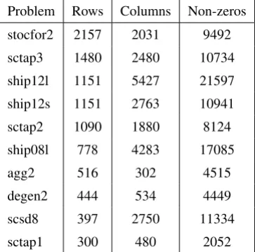
For computational illustration,Bregmanwas tested againstSaddleon ten lems from the Netlib library [17]. For the purpose of this comparison, each prob-lem was first cast in the form given in (77)-(79). Probprob-lem names and dimensions are given in Table 1.
All primal and dual variables are set to one initially. We set the perturbation step size parameters in (43)-(44) toλ =µ =0.5, the stepsize test parameters in (28) toγ = 0.3 andβ = 0.7. Two values for the stopping parameter were applied:φ =10−4andφ =10−6.
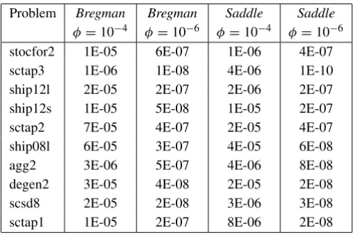
Table 2 shows the iteration count for φ = 10−4 and φ = 10−6, both for BregmanandSaddle. Table 3 shows the corresponding relative objective errors |ctx¯−ctx∗|/|ctx∗|, wherex¯is the primal solution obtained at the end of iterations
φ = 10−4andφ = 10−6, respectively). Due to function evaluations (for the exponent functions) and due to the search for step sizes, work per iteration for Bregmanis somewhat larger than for Saddle. The computational tests show that the performance ofBregmanappears quite equivalent toSaddle. One may speculate that a better scaling method forBregmanmay improve its performance.
Problem Rows Columns Non-zeros
stocfor2 2157 2031 9492
sctap3 1480 2480 10734
ship12l 1151 5427 21597
ship12s 1151 2763 10941
sctap2 1090 1880 8124
ship08l 778 4283 17085
agg2 516 302 4515
degen2 444 534 4449
scsd8 397 2750 11334
sctap1 300 480 2052
Table 1 – The number of rows, columns and non-zeros in the test problems.
Problem Bregman Bregman Saddle Saddle
φ=10−4 φ=10−6 φ=10−4 φ=10−6
stocfor2 29697 63289 11973 40605
sctap3 1761 3907 2726 5623
ship12l 6703 49554 4842 73510
ship12s 6973 43230 4489 51034
sctap2 7282 17456 8143 19574
ship08l 8931 39012 5576 39106
agg2 47023 49856 42997 46769
degen2 8260 31714 6119 32293
scsd8 8419 83400 45413 146610
sctap1 17860 38041 10946 30513
Problem Bregman Bregman Saddle Saddle φ=10−4 φ=10−6 φ=10−4 φ=10−6
stocfor2 1E-05 6E-07 1E-06 4E-07
sctap3 1E-06 1E-08 4E-06 1E-10
ship12l 2E-05 2E-07 2E-06 2E-07
ship12s 1E-05 5E-08 1E-05 2E-07
sctap2 7E-05 4E-07 2E-05 4E-07
ship08l 6E-05 3E-07 4E-05 6E-08
agg2 3E-06 5E-07 4E-06 8E-08
degen2 3E-05 4E-08 2E-05 2E-08
scsd8 2E-05 2E-08 3E-06 3E-08
sctap1 1E-05 2E-07 8E-06 2E-08
Table 3 – Relative error in the optimal objective function value.
For each iterationk, define relative primal and dual infeasibilities, denoted by ek
P andekD, respectively, as follows: ekP = max
i {0, (b−Ax k)
i/(|bi| +ǫik)},
eDk = max
j {0, (A t
yk−c)j/(|cj| +δjk)}.
Table 4 reports the final infeasibilities in terms of max{ekP, ekD}for Bregman andSaddle, withφ =10−6.
Problem Bregman Saddle
stocfor2 3E-05 3E-06
sctap3 2E-05 1E-05
ship12l 1E-05 3E-05
ship12s 3E-05 6E-06
sctap2 1E-05 9E-06
ship08l 8E-06 4E-04
agg2 1E-04 6E-04
degen2 1E-06 2E-06
scsd8 8E-05 4E-05
sctap1 1E-06 4E-06
To see the importance of scaling, we ranBregmanfor a dozen of smallNetlib problems without scaling for φ = 10−4. Five out our twelve test problems failed to converge in one million iterations, while for the others the number of iterations was increased by a factor ranging from 3 to 22 as compared with the scaled version.
Our convergence results apply if the scaling factors are updated during a pre-specified number of iterations only. To demonstrate that it pays off to update scaling until the end, we run our smallest problemsctap1 fixing scaling after 5000 iterations. As a result, the number of iterations is 26088, forφ =10−4, and 63631, forφ = 10−6. Hence, the iteration count almost doubles as compared with results forsctap1in Table 2. In conclusion, our theoretical results apply if scaling is fixed after a given number of iterations; however, it is plainly more efficient to update scaling factors until the termination criterion is met.
Finally, it is important to note that for small problems both of these approaches often turn out to be inefficient. Their comparative advantage is expected to appear for large-scale problems, and in particular, our method may be of interest for massively parallel computing.
REFERENCES
[1] D. Bertsekas and J.N. Tsitsiklis,Parallel and Distributed Computation: Numerical Methods. Prentice Hall, New Jersey (1989).
[2] L.M. Bregman, The relaxation method of finding the common points of convex sets and its application to the solution of problems in convex programming. USSR Computational Mathematics and Mathematical Physics,7(3) (1967), 200–217.
[3] Y. Censor, A.N. Iusem and S.A. Zenios, An interior point method with Bregman functions for the variational inequality problem with paramonotone operators. Mathematical Program-ming,81(1998), 373–400.
[4] Y. Censor and A. Lent, An iterative row-action method for interval convex programming. Journal of Optimization Theory and Applications,34(1981), 321–353.
[5] Y. Censor and S.A. Zenios, The proximal minimization algorithm withD-functions.Journal of Optimization Theory and Applications,73(1992), 451–464.
[6] G. Chen and M. Teboulle, Convergence analysis of a proximal-like optimization algorithm using Bregman functions.SIAM Journal on Optimization,3(1993) 538–543.
[8] J. Eckstein, Nonlinear proximal point algorithms using Bregman functions, with applications to convex programming.Mathematics of Operations Research,18(1993), 202–226. [9] P.T. Harker and J.S. Pang, Finite dimensional variational inequalities and nonlinear
comple-mentarity problems: a survey of theory, algorithms and applications. Mathematical Pro-gramming,48(1990), 161–220.
[10] A.N. Iusem, On some properties of generalized proximal point methods for quadratic and linear programming.Journal of Optimization Theory and Applications,85(1995), 593–612. [11] A.N. Iusem, An iterative algorithm for the variational inequality problem. Computational
and Applied Mathematics,13(1994), 103–114.
[12] A.N. Iusem, An interior point method for the nonlinear complementarity problem.Applied Numerical Mathematics,24(1997), 469–482.
[13] M. Kallio and A. Ruszczy´nski, Perturbation methods for saddle point computation. Working Paper 94-38, Institute for Applied Systems Analysis, Laxenburg, Austria (1994).
[14] M. Kallio and S. Salo, Tatonnement procedures for linearly constrained convex optimization. Management Science,40(1994), 788–797.
[15] E.N. Khobotov, Modifications of the extragradient method for solving variational inequalities and certain optimization problems. USSR Computational Mathematics and Mathematical Physics,27(5) (1987), 120–127.
[16] G.M. Korpelevich, The extragradient method for finding saddle points and other problems. Ekonomika i Matematcheskie Metody,12(1976), 747–756.
[17]LP Netlib, Test Problems, Bell Laboratories.
[18] R.T. Rockafellar, Local boundedness of nonlinear monotone operators. Michigan Mathe-matical Journal,16(1969), 397–407.
[19] R.T. Rockafellar,Convex Analysis. Princeton University Press, New Jersey (1970). [20] A.W. Tucker, Dual systems of homogeneous linear relations. InLinear Inequalities and