ACPD
15, 4823–4877, 2015NH3bi-directional
exchange
L. Zhu et al.
Title Page
Abstract Introduction
Conclusions References
Tables Figures
◭ ◮
◭ ◮
Back Close
Full Screen / Esc
Printer-friendly Version
Interactive Discussion
Discussion
P
a
per
|
Discussion
P
a
per
|
Discussion
P
a
per
|
Discussion
P
a
per
|
Atmos. Chem. Phys. Discuss., 15, 4823–4877, 2015 www.atmos-chem-phys-discuss.net/15/4823/2015/ doi:10.5194/acpd-15-4823-2015
© Author(s) 2015. CC Attribution 3.0 License.
This discussion paper is/has been under review for the journal Atmospheric Chemistry and Physics (ACP). Please refer to the corresponding final paper in ACP if available.
Global evaluation of ammonia
bi-directional exchange
L. Zhu1, D. Henze1, J. Bash2, G.-R. Jeong1,2, K. Cady-Pereira3, M. Shephard4, M. Luo5, F. Paulot6,7, and S. Capps2
1
Department of Mechanical Engineering, University of Colorado, Boulder, Colorado, USA 2
US Environmental Protection Agency, Research Triangle Park, North Carolina, USA 3
Atmospheric and Environmental Research, Inc., Lexington, Massachusetts, USA 4
Environment Canada, Toronto, Ontario, Canada 5
Jet Propulsion Laboratory, California Institute of Technology Pasadena, CA, USA 6
Program in Atmospheric and Oceanic Sciences, Princeton University, Princeton, New Jersey, USA
7
Geophysical Fluid Dynamics Laboratory/National Oceanic and Atmospheric Administration, Princeton, New Jersey, USA
Received: 7 December 2014 – Accepted: 27 January 2015 – Published: 20 February 2015
Correspondence to: D. Henze (daven.henze@colorado.edu)
ACPD
15, 4823–4877, 2015NH3bi-directional
exchange
L. Zhu et al.
Title Page
Abstract Introduction
Conclusions References
Tables Figures
◭ ◮
◭ ◮
Back Close
Full Screen / Esc
Printer-friendly Version
Interactive Discussion
Discussion
P
a
per
|
Discussion
P
a
per
|
Discussion
P
a
per
|
Discussion
P
a
per
|
Abstract
Bi-directional air–surface exchange of ammonia (NH3) has been neglected in many
air quality models. In this study, we implement the bi-directional exchange of NH3 in
the GEOS-Chem global chemical transport model. We also introduce an updated di-urnal variability scheme for NH3 livestock emissions and evaluate the recently devel-5
oped MASAGE_NH3 bottom up inventory. While updated diurnal variability improves
comparison of modeled-to-hourly in situ measurements in the Southeastern US, NH3 concentrations decrease throughout the globe, up to 17 ppb in India and Southeast-ern China, with corresponding decreases in aerosol nitrate by up to 7 µg m−3. The ammonium (NH+4) soil pool in the bi-directional exchange model largely extends the
10
NH3 lifetime in the atmosphere. Including bi-directional exchange generally increases
NH3 gross emissions (7.1 %) and surface concentrations (up to 3.9 ppb) throughout
the globe in July, except in India and Southeastern China. In April and October, it decreases NH3 gross emissions in the Northern Hemisphere (e.g., 43.6 % in April in
China) and increases NH3gross emissions in the Southern Hemisphere. Bi-directional 15
exchange does not largely impact NH+4 wet deposition overall. While bi-directional ex-change is fundamentally a better representation of NH3emissions from fertilizers,
emis-sions from primary sources are still underestimated and thus significant model biases remain when compared to in situ measurements in the US. The adjoint of bi-directional exchange has also been developed for the GEOS-Chem model and is used to
inves-20
tigate the sensitivity of NH3 concentrations with respect to soil pH and fertilizer
ACPD
15, 4823–4877, 2015NH3bi-directional
exchange
L. Zhu et al.
Title Page
Abstract Introduction
Conclusions References
Tables Figures
◭ ◮
◭ ◮
Back Close
Full Screen / Esc
Printer-friendly Version
Interactive Discussion
Discussion
P
a
per
|
Discussion
P
a
per
|
Discussion
P
a
per
|
Discussion
P
a
per
|
1 Introduction
Ammonia (NH3) is an important precursor of particulate matter (PM2.5) that harms
hu-man health (Reiss et al., 2007; Pope et al., 2009; Crouse et al., 2012) and impacts cli-mate through aerosol and short-lived greenhouse gas concentrations (Langridge et al., 2012). Global emissions of NH3have increased by a factor of 2 to 5 since pre-industrial 5
times, and they are projected to continue to rise over the next 100 years (Lamarque et al., 2011; Ciais, 2013). NH3 is an important component of the nitrogen cycle and accounts for a significant fraction of long-range transport (100’s of km) of reactive ni-trogen (Galloway et al., 2008). Excessive deposition of NH3 already threatens many
sensitive ecosystems (Liu et al., 2013).
10
Uncertainties in estimates of NH3emissions are significant. Surface-level NH3
mea-surements have been limited in spatial and temporal coverage, leading to large dis-crepancies in emissions estimates (Pinder et al., 2006). Additional information from remote sensing observations has been used to gain a better understanding of NH3
dis-tributions (Clarisse et al., 2009; Shephard et al., 2011; Pinder et al., 2011; Van Damme
15
et al., 2014). These observations have also been used as inverse modeling constraints on NH3 emissions (Zhu et al., 2013). While this approach leads to improved results
regarding the comparison of air quality model estimates to independent surface obser-vations in the US (Zhu et al., 2013), several limitations of this approach were identified. First, model biases in NHxwet deposition were not reduced. Emission constraints from 20
remote sensing measurements available only once per day were very sensitive to the model’s diurnal variation of NH3sources. Also, the remote sensing observations used in Zhu et al. (2013) are sparsely distributed, leading to a quantifiable sampling bias. Other inverse modeling studies of NH3 emissions have been performed using in situ
observations, such as aerosol SO24+ and NO−3 (Henze et al., 2009), aircraft
obser-25
ACPD
15, 4823–4877, 2015NH3bi-directional
exchange
L. Zhu et al.
Title Page
Abstract Introduction
Conclusions References
Tables Figures
◭ ◮
◭ ◮
Back Close
Full Screen / Esc
Printer-friendly Version
Interactive Discussion
Discussion
P
a
per
|
Discussion
P
a
per
|
Discussion
P
a
per
|
Discussion
P
a
per
|
model biases in HNO3(Heald et al., 2012; Zhang et al., 2012) or precipitation Paulot et al. (2014).
The modest success of previous inverse modeling studies suggests that updates to the dynamic and physical processes governing NH3are needed in addition to improve-ments in emissions estimates. Nighttime NH3concentrations are consistently overes-5
timated in many air quality models (e.g., GEOS-Chem, CMAQ). This may contribute to an overestimate of monthly averaged NH3 concentration following the assimilation of Tropospheric Emission Spectrometer (TES) observations (Zhu et al., 2013).
Another area in which many air quality models are currently deficient is in treatment of the air–surface exchange of NH3. Rigorous treatment of the bi-directional flux of
10
NH3 can substantially impact NH3deposition, emission, re-emission and atmospheric lifetime (Sutton et al., 2007). Re-emission of NH3 from soils can be a significant part
of NH3 sources in some regions. However, this bi-directional exchange mechanism is
neglected by many air quality models (e.g., GEOS-Chem). Several recent studies have begun to include resistance-based bi-directional exchange wherein the NH3flux direc-15
tion is determined by comparing the ambient NH3 concentration to the NH3in-canopy
compensation point. Sutton et al. (1998) and Nemitz et al. (2001) began with the air– canopy exchange model and extended the model by including air–soil exchange, but with no soil resistance. Cooter et al. (2010) and Bash et al. (2010) developed and extended the model to include a soil capacitance which assumes that NH3 and NH+4
20
exist in equilibrium in the soil. Bi-directional exchange of NH3coupled in a regional
air-quality model (Community Multiscale Air-Quality (CMAQ)) is evaluated in Bash et al. (2013) and Pleim et al. (2013).
Based on these previous studies, investigating the diurnal patterns of NH3
emis-sions and bi-directional air–surface exchange is critical for reducing uncertainties in the
25
GEOS-Chem model, which may in turn afford better top-down constraints NH3source distributions and temporal and seasonal variations. In this paper, we apply a new diur-nal distribution pattern to NH3livestock emissions in GEOS-Chem, which is developed
ACPD
15, 4823–4877, 2015NH3bi-directional
exchange
L. Zhu et al.
Title Page
Abstract Introduction
Conclusions References
Tables Figures
◭ ◮
◭ ◮
Back Close
Full Screen / Esc
Printer-friendly Version
Interactive Discussion
Discussion
P
a
per
|
Discussion
P
a
per
|
Discussion
P
a
per
|
Discussion
P
a
per
|
(CAFO) dominated areas in North Carolina (Bash et al., 2015). We then implement bi-directional exchange of NH3 in a global chemical transport model – GEOS-Chem
– following Pleim et al. (2013), and compare the model to in situ observations. As a first step towards including bi-directional exchange in NH3inverse modeling, we also develop the adjoint of bi-directional exchange in GEOS-Chem; this also provides a
use-5
ful method for quantifying the sensitivities of GEOS-Chem simulations with respect to important parameters in the bi-directional model, such as soil pH and fertilizer (only mineral fertilizer is considered in NH3 bi-directional exchange) application rate, which
are themselves uncertain.
Section 2 describes the model we use in this study. Section 3 introduces the in situ
10
observation networks we use for evaluation. The impacts of implementing the new di-urnal variation pattern of NH3emissions are presented in Sect. 4. The details of
devel-oping bi-directional exchange and its adjoint in GEOS-Chem are described in Sect. 5, followed by the evaluations and adjoint sensitivity analysis in Sect. 6. We present our conclusions in Sect. 7.
15
2 Methods
2.1 GEOS-Chem
GEOS-Chem is a chemical transport model driven with assimilated meteorology from the Goddard Earth Observing System (GEOS) of the NASA Global Modeling and As-similation Office (Bey et al., 2001). We use the nested grid of the model (horizontal
20
resolution 1/2◦×2/3◦) over the US and 2◦×2.5◦ horizontal resolution for the rest of the world. The year 2008 is simulated with a spin-up period of 3 months. The tropo-spheric oxidant chemistry simulation in GEOS-Chem includes a detailed ozone-NOx
-hydrocarbon-aerosol chemical mechanism (Bey et al., 2001) coupled with a sulfate-nitrate-ammonia aerosol thermodynamics module described in Park et al. (2004). The
25
ACPD
15, 4823–4877, 2015NH3bi-directional
exchange
L. Zhu et al.
Title Page
Abstract Introduction
Conclusions References
Tables Figures
◭ ◮
◭ ◮
Back Close
Full Screen / Esc
Printer-friendly Version
Interactive Discussion
Discussion
P
a
per
|
Discussion
P
a
per
|
Discussion
P
a
per
|
Discussion
P
a
per
|
The dry deposition of aerosols and gases scheme is based on a resistance-in-series model (Wesely, 1989), updated here to include bi-directional exchange (see Sect. 5).
Global anthropogenic and natural sources of NH3are from the GEIA inventory 1990
(Bouwman et al., 1997). The anthropogenic emissions are updated by the following regional inventories: the 2005 US EPA National Emissions Inventory (NEI) for US, the
5
Criteria Air Contaminants (CAC) inventory for Canada (van Donkelaar et al., 2008), the inventory of Streets et al. (2006) for Asia, and the Co-operative Program for Monitoring and Evaluation of the Long-range Transmission of Air Pollutants in Europe (EMEP) inventory for Europe (Vestreng and Klein, 2002). Monthly biomass burning emissions are from van der Werf et al. (2010), and biofuel emissions are from Yevich and Logan
10
(2003).
2.2 GEOS-Chem adjoint model
An adjoint model is an efficient tool for investigating the sensitivity of model estimates with respect to all model parameters simultaneously. This approach has been applied in recent decades in chemical transport models for source analysis of atmospheric
15
tracers (Fisher and Lary, 1995; Elbern et al., 1997) and for constraining emissions of tropospheric chemical species (Elbern et al., 2000). Adjoint models have also been used in air quality model sensitivity studies (e.g., Martien and Harley, 2006). The adjoint of GEOS-Chem is fully described and validated in Henze et al. (2007). It has been used for data assimilation using in situ observations (e.g., Henze et al., 2009; Paulot et al.,
20
2014) and remote sensing observations (e.g., Kopacz et al., 2010; Zhu et al., 2013; Xu et al., 2013). In this paper, we use the adjoint model to investigate the sensitivity of modeled NH3 with bi-directional exchange and a new diurnal distribution of NH3
ACPD
15, 4823–4877, 2015NH3bi-directional
exchange
L. Zhu et al.
Title Page
Abstract Introduction
Conclusions References
Tables Figures
◭ ◮
◭ ◮
Back Close
Full Screen / Esc
Printer-friendly Version
Interactive Discussion
Discussion
P
a
per
|
Discussion
P
a
per
|
Discussion
P
a
per
|
Discussion
P
a
per
|
3 Observations
3.1 Surface measurements
We use surface observations of NH3and wet deposited NH+4 from several networks to evaluate model estimates. The SouthEastern Aerosol Research and Characterization (SEARCH) network contains monitoring stations throughout the Southeast US. The
5
SEARCH network provides different sampling frequencies, such as daily, 3 day, 6 day, 1 min, 5 min and hourly, at different sites. Three monitoring stations (Oak Grove, MS, Jefferson Street, GA, and Yorkville, GA) provide 5 min long surface NH3observations.
We average the 5 min long observations of these three sites and convert them to be hourly average NH3concentration in July 2008.
10
The Ammonia Monitoring Network (AMoN) of National Atmospheric Deposition Pro-gram (NADP) contains 21 sites across the US with two-week long sample accumulation (Puchalski et al., 2011). We average the two-week long observations from Novem-ber 2007 through June 2010 to monthly NH3concentrations. The Interagency
Monitor-ing of Protected Visual Environments (IMPROVE) network (Malm et al., 2004) consists
15
of more than 200 sites in the continental US which collect PM2.5 particles over 24 h
every third day. We use monthly average sulfate and nitrate aerosols concentrations. We use wet NH+4 deposition observations from several monitoring networks around the world. The NADP National Trends Network (NTN) (http://nadp.sws.uiuc.edu/NTN) contains more than 200 sites in US which are predominately located in rural
ar-20
eas. It provides wet deposition observations of ammonium with week-long sample accumulation. The Canadian Air and Precipitation Monitoring Network (CAPMoN) (http://www.on.ec.gc.ca/natchem) contains about 26 sites which are predominately located in Central and Eastern Canada with 24 h integrated sample times. The Eu-ropean Monitoring and Evaluation Program (EMEP) (http://www.nilu.no/projects/ccc/
25
ACPD
15, 4823–4877, 2015NH3bi-directional
exchange
L. Zhu et al.
Title Page
Abstract Introduction
Conclusions References
Tables Figures
◭ ◮
◭ ◮
Back Close
Full Screen / Esc
Printer-friendly Version
Interactive Discussion
Discussion
P
a
per
|
Discussion
P
a
per
|
Discussion
P
a
per
|
Discussion
P
a
per
|
(EANET) (http://www.eanet.asia/product) contains 54 sites (21 urban, 13 rural, and 20 remote sites) with monthly observations of wet deposition of ammonium. We con-vert the daily/weekly/bi-weekly observations to monthly average NH+4 concentration in 2008.
4 Diurnal variability of ammonia livestock emission
5
4.1 Development of new diurnal distribution scheme
Simulated NH3surface concentrations in GEOS-Chem are significantly overestimated
at nighttime compared to hourly observations from the SEARCH network (Zhu et al., 2013). The standard NH3emissions in GEOS-Chem are evenly distributed throughout the 24 h of each day of the month, as indicated by the blue line in Fig. 1. That the
10
simulated NH3 emissions do not have any diurnal variation is a likely explanation for
this discrepancy with hourly observation. Thus, a new diurnal distribution scheme for NH3 livestock emissions has been developed in CMAQ (Bash et al., 2015). Here we
implement this algorithm in GEOS-Chem. The hourly NH3livestock emission,Eh(t), is
calculated from the monthly total emission,Em, as 15
Eh(t)=EmNmet(t), (1)
whereNmet(t) is the hourly fraction of the NH3 livestock emission during the month.
This depends on the aerodynamic resistance,Ra [s−1m], and surface temperature,T [K],
Nmet(t)=
H(t)/Ra(t)
Pn
t=1(H(t)/Ra(t))
, (2)
ACPD
15, 4823–4877, 2015NH3bi-directional
exchange
L. Zhu et al.
Title Page
Abstract Introduction
Conclusions References
Tables Figures
◭ ◮
◭ ◮
Back Close
Full Screen / Esc
Printer-friendly Version
Interactive Discussion
Discussion
P
a
per
|
Discussion
P
a
per
|
Discussion
P
a
per
|
Discussion
P
a
per
|
wherenis the number of hours in a month,tis the time during the month, from 1 ton, andH(t) is the Henry’s equilibrium, calculated following Nemitz et al. (2000),
H(t)=161 500
T e
−10 380/T, (3)
More details of the development of this diurnal variability scheme can be found in Bash et al. (2015).
5
4.2 Global distribution
We replace the standard GEOS-Chem livestock emissions, which are evenly dis-tributed for each hour of the day (static), with this new diurnal variability of livestock emissions that peaks in the middle of the day (dynamic) (Fig. 1). This also introduces daily variability of livestock emissions into the simulation, which is not considered in the
10
standard GEOS-Chem model. As the standard GEOS-Chem anthropogenic emissions do not distinguish the livestock emissions sector, we calculate the absolute NH3
live-stock emissions based on the fractions of livelive-stock emissions in anthropogenic emis-sions in the 2008 NEI.
Significant improvements are found when we compare surface NH3 concentrations 15
to SEARCH observations after implementing the dynamic diurnal emissions. The dy-namic case decreases the surface NH3 concentration relative to the static case by
several ppb at night and increases concentrations slightly (up to 1 ppb) in the day. This reduces the model mean bias by up to 2.9 ppb at night.
To apply the dynamic emissions scheme globally, we implement a new global
20
NH3 anthropogenic emissions inventory Magnitude And Seasonality of AGricultural
Emissions model (MASAGE_NH3, Paulot et al., 2014), which contains sector-specific emissions for different agriculture sources, such as livestock emissions (the standard GEOS-Chem NH3emissions do not clearly distinguish this sector). Figure 2 shows the
global distribution of surface NH3 concentrations from the GEOS-Chem static and dy-25
ACPD
15, 4823–4877, 2015NH3bi-directional
exchange
L. Zhu et al.
Title Page
Abstract Introduction
Conclusions References
Tables Figures
◭ ◮
◭ ◮
Back Close
Full Screen / Esc
Printer-friendly Version
Interactive Discussion
Discussion
P
a
per
|
Discussion
P
a
per
|
Discussion
P
a
per
|
Discussion
P
a
per
|
between the dynamic and the static cases. In general, the dynamic case decreases the monthly NH3 surface concentration throughout the world with significant changes in Southeast China and India in all three months, which can be up to 17.1 ppb in China in October and 12.1 ppb in India in April. There are also large decreases in the Eastern US (up to 3.3 ppb) and southeastern of South America.
5
The modeled Representative Volume Mixing Ratio (RVMR) (Shephard et al., 2011) underestimates the observed RVMR from TES in the US and most places of the globe (Shephard et al., 2011; Zhu et al., 2013). In this study, we also compare the mod-eled RVMR from static and dynamic cases to the TES RVMR. We calculate modmod-eled RVMR at the same time and locations of TES retrievals during 2006 through 2009.
10
We average the RVMRs at the 2◦×2.5◦grid resolution for each month (April, July, and October). The static RVMR underestimates the TES RVMR throughout the globe in all three months except in India and Southeastern China in April. With the new diur-nal variability scheme (dynamic case), the modeled RVMR increases in many places (e.g., Eastern China, Northern India, South America) and decreases in the Middle US
15
and Northern Europe. The differences between the dynamic and static RVMR are from
−1.5 to 1.6 ppb. These changes generally reduce differences between modeled and observed RVMR, while the differences are enhanced in a few locations, such as North-ern India in April. However, the magnitude of these changes are small compared to the differences (from −11.4 to 3 ppb) between the static RVMR and TES RVMR. We
20
are able to detect more obvious changes between the static and dynamic cases when focusing on a livestock source region (California) and a hotter day, during which the dynamic RVMR increases 3.4 ppb (Henze et al., 2015).
High biases of surface nitrate aerosol concentrations in GEOS-Chem are found in the US (e.g., Heald et al., 2012; Walker et al., 2012). Here we consider the impact of
25
dynamic NH3 livestock emissions on surface nitrate concentration in the US, as well
ACPD
15, 4823–4877, 2015NH3bi-directional
exchange
L. Zhu et al.
Title Page
Abstract Introduction
Conclusions References
Tables Figures
◭ ◮
◭ ◮
Back Close
Full Screen / Esc
Printer-friendly Version
Interactive Discussion
Discussion
P
a
per
|
Discussion
P
a
per
|
Discussion
P
a
per
|
Discussion
P
a
per
|
all three months, which can be as large as 7 µg m−3 in October. There are also large decreases in the Eastern US which can be up to 2.7 µg m−3 in July. In October, there are large decreases in the dynamic case in comparision to static case in Northern India (up to 3.9 µg m−3) and Europe (up to 2.4 µg m−3in Poland).
Investigating the impacts of dynamic NH3livestock emissions on nitrogen deposition 5
is also of interest. In Fig. 4, we show the global distribution of total nitrogen depo-sition (wet depodepo-sition of NH3, ammonium, HNO3 and nitrate, and dry deposition of
NH3, ammonium, NO2, PAN, N2O5, HNO3 and nitrate) from GEOS-Chem static and
dynamic cases in April, July, and October of 2008. The dynamic case decreases ni-trogen deposition in most places in the world, yet increases it in several locations.
10
The largest decrease of nitrogen deposition occurs in Northern India in April by up to 3.6 kg N ha−1month−1. The total amount of nitrogen deposition in India decreases by 8.6 % in April. Decreases in nitrogen deposition in the dynamic case occur in South-eastern China in all three months, with the total amount of nitrogen deposition in China decreasing by 4.7 % in April, 2.8 % in July, 3.1 % in October. The new diurnal
vari-15
ability scheme has more NH3 from livestock emissions emitted in the daytime, when
the boundary layer is thicker than nighttime. Typically, this lowers deposition largely at night. However, it may also be conducive to more export of NH3in the atmosphere dur-ing the day. Thus, slight increases of nitrogen in the dynamic cases occur downwind of regions with large NH3 sources in the base cases, such as increases in southeastern 20
Russia owing to enhanced NH3export from Eastern China.
5 Bi-directional exchange of NH3
5.1 Bi-directional flux calculation
The dry deposition scheme in the standard GEOS-Chem model is based on the resis-tance in series formulation of Wesely (1989), which only considers the unidirectional
25
ACPD
15, 4823–4877, 2015NH3bi-directional
exchange
L. Zhu et al.
Title Page
Abstract Introduction
Conclusions References
Tables Figures
◭ ◮
◭ ◮
Back Close
Full Screen / Esc
Printer-friendly Version
Interactive Discussion
Discussion
P
a
per
|
Discussion
P
a
per
|
Discussion
P
a
per
|
Discussion
P
a
per
|
actually be bi-directional. In this paper, we update the dry deposition of NH3to combine NH3 dry deposition from the atmosphere and emission from vegetation. A simplified
schematic of the updated air–surface exchange process of NH3 is shown in Fig. 5.
More details of this bi-directional scheme can be found in Cooter et al. (2010) and Pleim et al. (2013). The total air–surface exchange flux,Ft, is calculated as a function 5
of the gradient between the ambient NH3concentration in the first (surface) layer of the
model and the canopy compensation point (Bash et al., 2013; Pleim et al., 2013),
Ft=
Cc−Ca Ra+0.5Rinc
, (4)
whereCais the ambient NH3concentration of the first atmospheric layer of the model, Cc is the canopy compensation point (which is set at one half of the in-canopy resis-10
tance, since NH3 can come from either air or soil to the canopy, thus, splitting Rinc
symmetrically is appropriate), Ra is the aerodynamic resistance, and Rinc is the
in-canopy aerodynamic resistance. Ca> Cc will result in deposition from air to surface,
andCa< Ccwill result in emission from surface to air.Ccis calculated as (Bash et al.,
2013),
15
Cc=
Ca Ra+0.5Rinc +
Cst Rb+Rst+
Cg 0.5Rinc+Rbg+Rsoil
(Ra+0.5Rinc)−1+(Rb+Rst)−1+(Rb+Rw)−1+(0.5Rinc+Rbg+Rsoil)−1
, (5)
whereRb,Rbg,Rst,RsoilandRware the resistances at the quasi-laminar boundary layer
of leaf surface, the quasi-laminar boundary layer of ground surface, the leaf stomatal, soil and cuticle respectively.Ra,Rb,Rbg,Rst andRw are already defined and used in
the standard GEOS-Chem deposition scheme. Here we define and calculateRsoiland 20
Rinc following Pleim et al. (2013). Cst and Cg are the NH3 concentrations in the leaf
ACPD
15, 4823–4877, 2015NH3bi-directional
exchange
L. Zhu et al.
Title Page
Abstract Introduction
Conclusions References
Tables Figures
◭ ◮
◭ ◮
Back Close
Full Screen / Esc
Printer-friendly Version
Interactive Discussion
Discussion
P
a
per
|
Discussion
P
a
per
|
Discussion
P
a
per
|
Discussion
P
a
per
|
et al., 2000).
Γ =[NH
+ 4]
[H+] . (6)
Γst is calculated as a function of land cover type, and the values of different land
cover types are based on Zhang et al. (2010). Γg is calculated as a function of soil pH and NH+4 concentration in the soil, [NH+4]soil. Soil pH data is taken from ISRIC – 5
World Soil Information with a 0.5◦×0.5◦ global resolution (http://www.isric.org/data/ data-download). We model the [NH+4]soil as an ammonium pool in the soil, which is a function of fertilizer application rate, deposition, nitrification, soil moisture, and emis-sion in bi-directional exchange. The calculation of [NH+4]soil is described in the next
section.
10
To compare the deposition (downward) flux and emission (upward) flux of the bi-directional case to the base case, we define diagnostic variables for gross deposition fluxFdepand emission fluxFemisas follows (Bash et al., 2013; Jeong et al., 2013),
Fdep=
Cc−Ca Ra+0.5Rinc
|Cst=0,Cg=0, (7)
Femis=
Cc Ra+0.5Rinc
|Ca=0, (8)
15
whereFdep is calculated under the assumption that there is no NH3emission potential
from the soil and canopy, andFemis is calculated under the assumption that there is no
NH3in the atmosphere. Thus,Fdep+Femis=Ft.
5.2 Soil ammonium pool
Here we introduce a NH+4 pool to track the NH3and NH+4 in the atmosphere and in the 20
soil. The inputs to the ammonium pool in the soil are NHx (NH3and NH+4) deposition
ACPD
15, 4823–4877, 2015NH3bi-directional
exchange
L. Zhu et al.
Title Page
Abstract Introduction
Conclusions References
Tables Figures
◭ ◮
◭ ◮
Back Close
Full Screen / Esc
Printer-friendly Version
Interactive Discussion
Discussion
P
a
per
|
Discussion
P
a
per
|
Discussion
P
a
per
|
Discussion
P
a
per
|
annual N fertilizer application rates are from Potter et al. (2010), which has chemical fertilizer (global total 70 Tg N yr−1) with a 0.5◦×0.5◦ resolution for the year 2000. We assume that all forms of N fertilizers will convert to NH+4 rapidly after fertilizer appli-cation. This dataset is also used to develop the global soil nitric oxide emissions in GEOS-Chem in Hudman et al. (2012). We use the same treatment of annual total
fer-5
tilization as Hudman et al. (2012) to derive daily fertilizer application rates by applying 75 % of the annual total fertilization amount around the first day of the growing sea-son (green-up day), distributed with a Guassian distribution one month after. The other 25 % is evenly distributed over the remaining time before the end of the growing sea-son (brown-down day). The determination of green-up and brown-down days is based
10
on the growing season dates derived from the MODIS Land Cover Dynamics product (MCD 12Q2) using the MODIS enhanced vegetation index (EVI) (Hudman et al., 2012). Using the fertilizer inputs described above, in addition to inputs from deposition and outputs from emission, the time dependent soil NH+4 pool [mol L−1] is calculated as
[NH+4]soil=[NHx]dep dsθNA
+ [N]fert
dsθMN
−[NH3]bidi emit
dsθNA
, (9)
15
where [NHx]dep [molec cm− 2
] is deposition from wet and dry deposition of NH3 and
NH+4, [N]fert [N g m− 2
] is the NH+4 from fertilizer, [NH3]bidi emit [molec cm− 2
] is the gross NH+4 emitting from the soil due to bi-directional exchange, MN is the molar mass of nitrogen, ds is the depth of the soil layer, taken to be 0.02 m, θ is the soil wetness
[m3m−3], andNAis Avogadro’s number. We then solve the mass balance equation for 20
[NHx]depand [N]fert,
d[NHx]dep
dt =Sdep−
[NHx]dep
τ −Ldep, (10)
d[N]fert
dt =Sfert− [N]fert
ACPD
15, 4823–4877, 2015NH3bi-directional
exchange
L. Zhu et al.
Title Page
Abstract Introduction
Conclusions References
Tables Figures
◭ ◮
◭ ◮
Back Close
Full Screen / Esc
Printer-friendly Version
Interactive Discussion
Discussion
P
a
per
|
Discussion
P
a
per
|
Discussion
P
a
per
|
Discussion
P
a
per
|
whereτ is the decay time owing to nitrification rate of NH+4 in soil. We assume τ is 15 days, since almost all NH+4 will convert to NO−3 within that timespan (Matson et al., 1998).Sdep is the deposition rate, Sfert is the fertilizer application rate, andLdep is the
deposition loss rate. We use the same assumption as Hudman et al. (2012) that only 60 % of this deposited NHx will enter the soil, while the rest of the NHx deposition will 5
runoff into waterways. Here we do not consider the production of NH+4 from NO−3 in the nitrogen cycle from mineralization nor immobilization. The time scale of these pro-cesses can be years, which is much larger than the time scale of the NH+4 simulations considered here; Cooter et al. (2010) also found these processes were not needed to accurately simulate NH3over managed lands on similar time scales.
10
5.3 Adjoint of bi-directional exchange
To investigate the sensitivity of modeled NH3 concentrations to the parameters in the
bi-directional exchange model, and to facilitate future inverse modeling, we develop the adjoint of our updated NH3flux scheme. Here we consider two key parameters, soil pH
and fertilizer application rate, since their values are highly approximate.
15
The adjoint sensitivity is defined as
λσ=
∂J(NH3)
∂σ , (12)
whereJ (NH3) is the total mass of ammonia at surface level in each grid box during 1 week. The unit ofJ (NH3) is kg box−
1
.σ in this study is defined as the soil pH scaling factor (σpH) or fertilizer application rate scaling factor (σfert_rate).σpH is defined as
pH pH0 20
andσfert_rateis defined as
fert_rate fert_rate0. pH
0
ACPD
15, 4823–4877, 2015NH3bi-directional
exchange
L. Zhu et al.
Title Page
Abstract Introduction
Conclusions References
Tables Figures
◭ ◮
◭ ◮
Back Close
Full Screen / Esc
Printer-friendly Version
Interactive Discussion
Discussion
P
a
per
|
Discussion
P
a
per
|
Discussion
P
a
per
|
Discussion
P
a
per
|
5.4 Validating the adjoint of bi-directional exchange
We validate the accuracy of the adjoint model by comparing the sensitivity of NH3
surface concentrations with respect to soil pH and fertilizer application rate calculated using the adjoint model with sensitivities calculated using the finite differences method. In order to make such comparisions efficiently throughout the model domain, horizontal
5
transport is turned off for these tests (e.g., Henze et al., 2007). Figure 6 shows the comparison of sensitivities calculated by adjoint and finite difference. The cost function is evaluated once at the end of a one week simulation. The slope of a linear regression and square of correlation coefficient, R2, are both close to unity, demonstrating the accuracy of adjoint of the bi-directional model.
10
6 Results and discussion
For the US region, we use nested horizontal resolution (1/2◦×2/3◦) simulations with the standard set of GEOS-Chem emission inventories. For the global simula-tion, we introduce a new bottom up emission inventory for NH3 agriculture sources, MASAGE_NH3 (Paulot et al., 2014). The full description of the differences between
15
the GESO-Chem standard NH3 emission inventories and MASAGE_NH3 is in Paulot
et al. (2014). We perform global simulation at a horizontal resolution of 2◦×2.5◦. All sim-ulations include the dynamic treatment of the diurnal variability of livestock emissions described in Sect. 4.
6.1 US
20
We run the GEOS-Chem model for April, July, and October of 2008 with the updated diurnal variation of NH3 livestock emissions and the bi-directional exchange
mecha-nism. Figure 7 shows the NH3total gross emissions from GEOS-Chem with (BIDI) and
without (BASE) the bi-directional air–surface exchange. The total gross emissions of BIDI case are the sum of primary emissions and upward fluxes from soil and
ACPD
15, 4823–4877, 2015NH3bi-directional
exchange
L. Zhu et al.
Title Page
Abstract Introduction
Conclusions References
Tables Figures
◭ ◮
◭ ◮
Back Close
Full Screen / Esc
Printer-friendly Version
Interactive Discussion
Discussion
P
a
per
|
Discussion
P
a
per
|
Discussion
P
a
per
|
Discussion
P
a
per
|
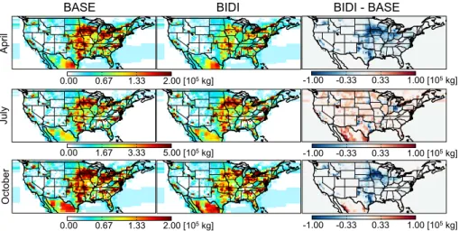
tion. Bi-directional exchange generally increases gross emissions in most parts of the US in July (up to 0.43 Gg month−1) and decreases gross emissions throughout the US in October (up to 0.29 Gg month−1). Significant decreases occur in the Great Plains region in both April and October with a magnitude of up to 0.23 Gg month−1 in April and 0.29 Gg month−1in October. Bi-directional exchange does not much alter the total
5
modeled emissions in the US in July (increase by 5.9 %) and October (decrease by 13.9 %), but does lead to a decrease of 23.3 % in April. With the ammonium soil pool, the model can preserve ammonia/ammonium in the soil rather than emitting it directly after fertilizer application. This is the main reason that gross emissions decrease in the Great Plains in April and October. In July, there is not as much fertilizer applied as
10
in April. However, the bi-directional exchange between the air and surface can induce NH3 to be re-emitted from the ammonium soil pool which reserve ammonium from
previous deposition and fertilizer application.
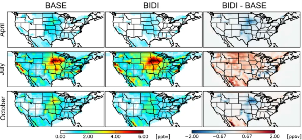
The spatial distributions of surface NH3concentrations in GEOS-Chem are shown in Fig. 8. In general, bi-directional exchange decreases monthly NH3surface concentra-15
tions in April (up to 1.8 ppb) and October (up to 2.1 ppb), and increases it in July (up to 2.8 ppb) throughout the US. There are peak decreases in NH3surface concentrations in the Great Plains in both April and October and increases in California in July. These changes of surface NH3 concentration are consistent with the pattern of changes to
NH3emissions in Fig. 7.
20
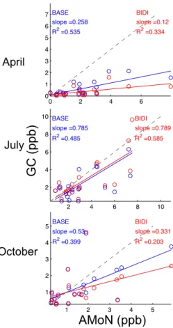
6.1.1 Evaluation with NH3
We evaluate the GEOS-Chem simulation with bi-directional exchange by comparing the model values to in situ observations from AMoN. Figure 9 shows the comparison of GEOS-Chem surface NH3concentrations in the BASE and BIDI cases with AMoN ob-servations. Bi-directional exchange decreases the normalized mean bias (NMB) from
25
ACPD
15, 4823–4877, 2015NH3bi-directional
exchange
L. Zhu et al.
Title Page
Abstract Introduction
Conclusions References
Tables Figures
◭ ◮
◭ ◮
Back Close
Full Screen / Esc
Printer-friendly Version
Interactive Discussion
Discussion
P
a
per
|
Discussion
P
a
per
|
Discussion
P
a
per
|
Discussion
P
a
per
|
R2 values increase by 20.6 % in July, and decrease by 37.6 % in April and 49.1 % in October. The slope slightly increases by 0.5 % in July, and decreases by 53.5 % and 37.5 % in April and October, respectively. The changes in slopes can also be seen in Fig. 8 as bi-directional exchange decreases the NH3monthly average concentration at
AMoN sites in April and October while it increases the NH3monthly average concen-5
trations in July. Modeled surface NH3 concentrations are significantly lower than the AMoN observations in April and October by a factor of 2–5, which is not unreason-able given likely underestimates in primary emissions (Zhu et al., 2013; Nowak et al., 2012; Schiferl et al., 2014). Such large underestimation is not corrected by applying the NH3 bi-directional exchange to the model. Other improvements in the model besides 10
bi-directional exchange, such as updating primary NH3emissions, are also required for
better estimating NH3surface concentrations.
6.1.2 Evaluation with aerosol nitrate
We also compare the simulated nitrate aerosol concentrations to the aerosol observa-tions from IMPROVE. Figure 10 shows the simulated monthly average nitrate aerosol
15
surface concentration from the GEOS-Chem BASE and BIDI cases in comparison to IMPROVE observations in 2008. GEOS-Chem overestimates nitrate in the BASE case in all three months. The overestimates in BASE cases can be 5 times larger in October. Bi-directional exchange generally decreases the nitrate concentrations in April, which makes the slope of the regression line decrease by 45.4 %. However there are still
20
large overestimates (∼a factor of 2 on average) in the Northeast US and large under-estimates (up to 1.7 µg m−3) in South California in the BIDI case in April. Bi-directional exchange slightly increases (less than 0.5 µg m−3) nitrate in July and decreases (less than 0.4 µg m−3) nitrate in October, which does not significantly impact the comparison of modeled nitrate with IMPROVE observations.
25
ACPD
15, 4823–4877, 2015NH3bi-directional
exchange
L. Zhu et al.
Title Page
Abstract Introduction
Conclusions References
Tables Figures
◭ ◮
◭ ◮
Back Close
Full Screen / Esc
Printer-friendly Version
Interactive Discussion
Discussion
P
a
per
|
Discussion
P
a
per
|
Discussion
P
a
per
|
Discussion
P
a
per
|
et al., 2013). Heald et al. (2012) recommend that reducing the nitric acid to 75 % would bring the magnitude of nitrate aerosol concentration into agreement with the IMPROVE observations. In our study, based on the comparison of BASE modeled nitrate concen-tration and IMPROVE observation, we perform sensitivity studies by reducing the nitric acid to 50 % in July and to 20 % in October at each timestep in the GEOS-Chem model
5
for both BASE and BIDI cases. Modeled nitrate concentrations reduce dramatically with this adjustment in July and October, but overestimates still exist in many places in the Eastern US We also compare the modeled NH3 surface concentrations in the
sensitivity simulations with adjusted nitric acid concentrations to the AMoN observa-tions, since reducing the nitric acid in the model may cause NH3 to partition more to
10
the gas phase, which could bring modeled NH3 concentrations into better agreement with AMoN observations. However, no significant impacts are found in NH3
concentra-tions at AMoN site locaconcentra-tions with these nitric acid adjustments, consistent with earlier assessments that the model’s nitrate formation is NH3 limited throughout much of the US (Park et al., 2004). Overall, overestimation of model nitrate by a factor of 3 to 5
15
appears to be a model deficiency beyond the issue of NH3bi-directional exchange.
6.1.3 Comparison to inverse modeling
Inverse modeling estimates of uni-directional NH3 emissions using TES observations lead to overestimates of ammonia concentration in comparison to surface observations from AMoN in July (Zhu et al., 2013), and emissions estimates in July are much higher
20
than other top-down or bottom up studies (Paulot et al., 2014). It is thus of interest to evaluate whether bi-directional exchange of NH3would reduce this high bias. Although
repeating the inverse modeling with TES NH3observations and bi-directional exchange
is beyond the scope of this work, we can use the optimized emissions from Zhu et al. (2013) as the basis upon which bi-directional exchange is applied. Figure 11 shows
25
the modeled NH3monthly average surface concentrations in comparison to the AMoN
ACPD
15, 4823–4877, 2015NH3bi-directional
exchange
L. Zhu et al.
Title Page
Abstract Introduction
Conclusions References
Tables Figures
◭ ◮
◭ ◮
Back Close
Full Screen / Esc
Printer-friendly Version
Interactive Discussion
Discussion
P
a
per
|
Discussion
P
a
per
|
Discussion
P
a
per
|
Discussion
P
a
per
|
are from GEOS-Chem with NH3bi-directional exchange using the optimized emissions from Zhu et al. (2013). The model with bi-directional exchange decreases the high bias in July: the NMB decreases by 80.4 %; the RMSE decreases by 56.7 %. TheR2 value increases by 43.3 %. However, the model with bi-directional exchange now un-derestimates the NH3monthly average concentrations in April and October. The RMSE 5
increases by 4.1 % in April and 28.8 % in October. The impacts of NH3 concentration
with respect to emissions in the model with bi-directional exchange are nonlinear. Us-ing the optimized NH3 emissions inventories from the TES NH3 assimilation with the
BASE model does not guarantee a better estimation of NH3 surface concentrations
with the BIDI model. Therefore, full coupling of inverse modeling with TES NH3
obser-10
vations and bi-directional exchange is necessary. Also, investigating the sensitivities of bi-directional model results to the NH3emissions, as well as other critical parameters,
is important for improving the NH3concentration estimation.
6.2 Global modeling results
While bi-directional exchange of NH3 has previously been implemented in regional 15
models (e.g., Bash et al., 2013; Zhang et al., 2010; Wichink Kruit et al., 2012), with the GEOS-Chem model we have the chance to evaluate NH3 bi-directional exchange on global scales for the first time. The global distribution of NH3 gross emissions in both BASE and BIDI cases, as well as their differences, are shown in Fig. 12. Gen-erally, bi-directional exchange decreases NH3emissions in the Northern Hemisphere, 20
and increases NH3 gross emissions in the Southern Hemisphere in April and Octo-ber. Total NH3emissions in the Northern Hemisphere decrease by 22.6 % in April and
7.8 % in October. In July, bi-directional exchange increases NH3 emissions in most
places (7.1 % globally), except China and India. Significant decreases in NH3 emis-sions in the BIDI case occur in Southeastern China and Northern India in all three
25
ACPD
15, 4823–4877, 2015NH3bi-directional
exchange
L. Zhu et al.
Title Page
Abstract Introduction
Conclusions References
Tables Figures
◭ ◮
◭ ◮
Back Close
Full Screen / Esc
Printer-friendly Version
Interactive Discussion
Discussion
P
a
per
|
Discussion
P
a
per
|
Discussion
P
a
per
|
Discussion
P
a
per
|
28.8 % in April, 22.8 % in July, and 7.2 % in October. There are also large decreases of total NH3emissions in the US, Mexico and Europe in April of up to 6.5 Gg month
−1
. The changes of NH3 gross emissions between BASE and BIDI cases can be seen
more directly from the comparison of fertilizers emissions in the BASE case with those in the BIDI case. In Fig. 13, we show the global distribution of NH3fertilizer emissions in 5
the BASE and BIDI cases. In BIDI case, the fertilizer emissions are the upward fluxes from soil and vegetation from bi-directional exchange. The third column is the NH3 emissions from all other sources except fertilizers in April, July, and October of 2008. In the BASE case, fertilizers emissions have peak values in Eastern China and Middle East Asia and much smaller values elsewhere. Fertilizers emissions in the BIDI case
10
increase in many places where there are no or near zero values in the BASE case. In the BIDI case, the fertilizer emissions distribution is much more homogeneous. As we described in Sect. 6.1, fertilizer emissions are lower in the BIDI case under cool spring and fall time conditions due to the temperature effects on NH3 emissions and storage in the soil ammonium pool. The deposition and re-emission processes in bi-directional
15
exchange model thus extend the effect of NH3 emissions from fertilizers. There are
obvious trends that fertilizer emissions in the Northern Hemisphere are larger than those in the Southern Hemisphere in spring and summer, and fertilizer emissions in the Southern Hemisphere are larger than those in the Northern Hemisphere in fall. The global amount of NH3fertilizer emissions is 27.8 % of total emissions from all sources
20
in the BASE case and 12.8 % in the BIDI case in April.
Figure 14 shows the global distribution of NH3 monthly surface concentrations in
the BASE and BIDI cases and their differences in April, July and October. In gen-eral, bi-directional exchange increases NH3 concentrations throughout the world in
July by up to 3.9 ppb. It decreases NH3 concentrations in the Northern Hemisphere 25
(up to 27.6 ppb) and increases NH3 concentrations in the Southern Hemisphere (up to 4.2 ppb) in April and October. Significant decreases of NH3concentrations occur in
ACPD
15, 4823–4877, 2015NH3bi-directional
exchange
L. Zhu et al.
Title Page
Abstract Introduction
Conclusions References
Tables Figures
◭ ◮
◭ ◮
Back Close
Full Screen / Esc
Printer-friendly Version
Interactive Discussion
Discussion
P
a
per
|
Discussion
P
a
per
|
Discussion
P
a
per
|
Discussion
P
a
per
|
this study, were higher than the bottom-up NH3emissions from Huang et al. (2012) in China in April and July, and similar to the emissions from Streets et al. (2003) in April, July, and October. Overestimation of NH3 surface concentrations in GEOS-Chem in
China are found in Wang et al. (2013) when using NH3 emissions from Streets et al. (2003), leading to an overestimation of nitrate aerosol concentrations in China.
Obser-5
vations from IASI have discrepancies over China with NH3 concentrations in
GEOS-Chem (Kharol et al., 2013; Clarisse et al., 2009) that may in part be improved by the impacts of bi-directional exchange. However, observations from TES show NH3
con-centrations in GEOS-Chem (with NH3emissions from Streets et al., 2003) are
under-estimated in many places of the globe including China (Shephard et al., 2011). We
10
must note that the lower NH3concentrations presented here are daily averages, while IASI and TES data are for a particular hour of the day. The changes in the emissions profile may reduce the model underestimate against the satellite observations while decreasing the mean NH3concentrations.
6.3 Wet deposition evaluation (global and US)
15
We compare the model NH+4 wet deposition to in situ observations in several regions of the world using NTN for the continental US, CAPMoN for Canada, EMEP for Europe, and EANET for East Asia, see Fig. 15. For the model NH+4 wet deposition, we also include the model NH3 wet deposition since NH+4 wet deposition from in situ
observa-tions includes precipitated NH3. Since there are biases in the modeled precipitation, 20
we scale the model wet deposition by multiplying the modeled deposition by the ratio of the observed to modeled precipitation, Fluxmodel·(
Pobs Pmodel)
0.6
, following the correction
method in Paulot et al. (2014). We only include observations that have 0.25<Pobs Psim <4 to
limit the effect of this correction (Paulot et al., 2014), and we also exclude observations which are beyond three times the standard deviation of observed NH+4 wet deposition
25
ACPD
15, 4823–4877, 2015NH3bi-directional
exchange
L. Zhu et al.
Title Page
Abstract Introduction
Conclusions References
Tables Figures
◭ ◮
◭ ◮
Back Close
Full Screen / Esc
Printer-friendly Version
Interactive Discussion
Discussion
P
a
per
|
Discussion
P
a
per
|
Discussion
P
a
per
|
Discussion
P
a
per
|
In general, the GEOS-Chem model underestimates NH+4 wet deposition throughout the world in the BASE case. Large increases in NH+4 wet deposition in the BIDI cases are found in the US, Canada, and Europe in July (up to 6.31 kg ha−1yr−1). The slopes of the regression line when compared to observations increase by 37.9 % in US, 54.9 % in Canada, and 17.7 % in Europe in the BIDI cases in July, all becoming closer to unity.
5
However, the bi-directional exchange increases the RMSE by 64.3 % in the US, 37.2 % in Canada, and 36.0 % in Europe.
Bi-directional exchange does not impact the NH+4 wet deposition much in April and October. It decreases NH+4 wet deposition slightly (up to 3.77 kg ha−1yr−1in Europe) at most of the observation locations in the US, Canada, and Europe in April. The slopes
10
decrease by 14.3 % in the US, 6.8 % in Canada, and 12.3 % in Europe. Bi-directional exchange decreases the NMB by 46.4 % in the US, 37.6 % in Europe in April, but increases the NMB by 28.3 % in Canada, and 11.6 % in East Asia. In October, bi-directional exchange increases NH+4 wet deposition slightly at most of the observation locations (up to 3.85 kg ha−1yr−1). The changes in RMSE between BASE and BIDI
15
cases are small, less than 10 %.
The overall differences of NH+4 wet deposition between the BASE and BIDI cases are generally small (from−4.95 to 6.31 kg ha−1yr−1), even when the differences in NH3
emissions are substantial. For example, total NH3 emissions decrease by 43.6 % in China in April with bi-directional exchange, but changes in NH+4 wet deposition are
20
not very large (from−4.95 to 2.52 kg ha−1yr−1). While implementing NH3bi-directional
ACPD
15, 4823–4877, 2015NH3bi-directional
exchange
L. Zhu et al.
Title Page
Abstract Introduction
Conclusions References
Tables Figures
◭ ◮
◭ ◮
Back Close
Full Screen / Esc
Printer-friendly Version
Interactive Discussion
Discussion
P
a
per
|
Discussion
P
a
per
|
Discussion
P
a
per
|
Discussion
P
a
per
|
6.4 Adjoint sensitivity analysis
6.4.1 Global adjoint sensitivities
In Sect. 5.3, we demonstrated the accuracy of the sensitivities calculated using the adjoint of the GEOS-Chem bi-directional model. In this section, we present the adjoint sensitivities of NH3 surface concentrations with respect to the important parameters 5
in the bi-directional model. Figure 16 shows the adjoint sensitivities of NH3 surface concentration with respect to the scaling factors for the soil pH (left) and for the fertilizer application rate (right) in April, July, and October 2008. The sensitivities with respect to both parameters are always positive throughout the globe. Sensitivities of NH3 to fertilizer application rate are positive as excess fertilizer application will increase the
10
NH3 soil emission potential. Sensitivities of NH3 to soil pH are also positive as low
H+ concentrations in soil (high soil pH) increases dissociation of NH+4 to NH3, thereby increasing the potential for volatilization of NH3.
The relationship between NH3concentration and soil pH is stronger during the
grow-ing season since more ammonium is in the soil pool. Slight changes in pH may have
15
large impacts on the amount of NH3 emitted from soil and further induce large diff
er-ences in NH3surface concentrations. As we can see in the left column of Fig. 16, the
sensitivities of NH3 surface concentrations with respect to soil pH scaling factors are larger in the Northern Hemisphere than those in the Southern Hemisphere in April and July, and less in the Northern Hemisphere than those in the Southern Hemisphere in
20
October, since the growing seasons are in April in the Northern Hemisphere and in October in the Southern Hemisphere. Large sensitivities in July in the Northern Hemi-sphere are due to ammonium in the soil pool accumulated from CAFO emissions via deposition. However, some caution is warranted in interpreting the seasonality of these sensitivities, as our model does not include any seasonal variations in soil pH.
Sea-25
sum-ACPD
15, 4823–4877, 2015NH3bi-directional
exchange
L. Zhu et al.
Title Page
Abstract Introduction
Conclusions References
Tables Figures
◭ ◮
◭ ◮
Back Close
Full Screen / Esc
Printer-friendly Version
Interactive Discussion
Discussion
P
a
per
|
Discussion
P
a
per
|
Discussion
P
a
per
|
Discussion
P
a
per
|
mer (Slattery and Ronnfeldt, 1992). Variation of soil pH can be more than one unit from spring to fall (Angima, 2010), thus the uncertainty in the constant annual soil pH used here could be about 20 % owing to neglecting seasonality.
The relationship between NH3 concentration and fertilizer application rate is also seasonally dependent. The seasonal trends of sensitivities of NH3 to fertilizer appli-5
cation rate are similar to sensitivities of NH3 to soil pH. Larger sensitivities appear
in places with lower fertilizer application rates than those with plenty of fertilizer. For example, the largest fertilizer application rates appear in Southeast China, Northwest Europe and Northern India in April, and sensitivities are nearly zero in each of these locations. That the magnitude of the fertilizer application rates itself is an important
10
factor in determining the sensitivities of NH3 concentration to the fertilizer application rate is indicative of the nonlinear relationship introduced by treatment of bi-directional exchange.
Through investigating the sensitivities of NH3 surface concentration to the soil pH and the fertilizer application rate, we know that NH3 surface concentrations are very 15
sensitive to these parameters in many places of globe. We also find that NH3surface
concentrations are more sensitive to soil pH than fertilizer application rate in general. In addition to the adjoint sensitivity analysis of NH3 concentrations to the soil pH and
the fertilizer application rate, it is also interesting to know the ranking of sensitivities of NH3 concentrations with respect to other parameters, such as NH3 concentrations at
20
compensation points (Cc,Cst,Cg), NH3 emission potentials (Γg,Γst), and resistances
(Ra,Rinc, Rsoil,Rg,Rst,Rbg,Rw). Knowledge of the sensitivity of NH3 concentrations
with respect to these parameters may help improve the model estimation of the spatial and temporal distributions as well as the magnitudes of NH3concentrations.
6.4.2 Comparison to in situ NH3with adjusted BIDI parameters 25
ACPD
15, 4823–4877, 2015NH3bi-directional
exchange
L. Zhu et al.
Title Page
Abstract Introduction
Conclusions References
Tables Figures
◭ ◮
◭ ◮
Back Close
Full Screen / Esc
Printer-friendly Version
Interactive Discussion
Discussion
P
a
per
|
Discussion
P
a
per
|
Discussion
P
a
per
|
Discussion
P
a
per
|
model. It is interesting to explore to what extent biases in the modeled NH3
concentra-tions may be explained by uncertainties in the parameters of the bi-directional model, rather than e.g., revising livestock NH3emissions. To test this, we increase the soil pH
value by a factor of 1.1, since uncertainties of seasonal soil pH are about 20 %. As expected, the NH3 surface concentrations generally increase over the globe (e.g., up
5
to 3.4 ppb in April). Large increases occur in places with large sensitivities to soil pH (Fig. 16, upper right). NH3concentrations are underestimated in the model in
compar-ison to the AMoN observations in the US. They are also underestimated in many parts of globe in comparison to TES observations (Shephard et al., 2011). With this adjust-ment to soil pH, the discrepancy between TES observations and the model in upper
10
levels of the boundary layer may potentially be reduced in regions where GEOS-Chem NH3is underestimated before the growing seasons and overestimated after the
grow-ing seasons. Slight increases in NH3surface concentrations are found throughout the
US as NH3is not very sensitive to soil pH in the US (see Fig. 16). Thus, this adjustment does not improve the comparison to AMoN observations in the US.
15
In this study, we did not consider the adjustment of soil pH in agricultural areas by the farmers who limit the soil pH in a certain range to improve crop yield (Haynes and Naidu, 1998). However, no significant changes in the modeled surface NH3
concen-trations occur with bi-directional exchange when we limit the soil pH in the agricultural areas between 5.5 and 6.5 (generally less than 1 ppb over the globe, up to 3.4 ppb in
20
India), since sensitivities are not very strong in the agricultural areas (see left column of Fig. 16).
Small differences between bi-directional and unidirectional fluxes in the US are also indicated in Dennis et al. (2013), wherein sensitivity tests were performed varying the soil emission potential (Γg, a parameter which includes both soil pH and fertilizer appli-25
ACPD
15, 4823–4877, 2015NH3bi-directional
exchange
L. Zhu et al.
Title Page
Abstract Introduction
Conclusions References
Tables Figures
◭ ◮
◭ ◮
Back Close
Full Screen / Esc
Printer-friendly Version
Interactive Discussion
Discussion
P
a
per
|
Discussion
P
a
per
|
Discussion
P
a
per
|
Discussion
P
a
per
|
From Zhu et al. (2013), we know that the underestimation of NH3 emissions in the unidirectional model can be as much as a factor of 9 in the US. We also notice that NH3
may not change much when fertilizer emissions increase a lot in regions such as Mid-west US and Northern Australia (see Figs. 13 and 14). Thus, low emissions from other sources, such as livestock, may be a big part of the reason for underestimating NH3 5
concentrations in the bi-directional exchange model. To better understand this, we also test increasing NH3livestock emissions by a factor of 8 in April and 3 in October as NH3 concentrations are generally underestimated by around 8 and 3 times (Fig. 9) compare to AMoN observations in April and October, respectively. These adjustments bring the NH3concentrations into a much better agreement with the magnitude of AMoN
obser-10
vations, see Fig. 17. However, uniformly increasing the livestock emissions does not well represent the NH3spatial distribution with the AMoN observations (correlations of
model and observation are very low). Overall, treatment of bi-directional exchange can improve our understanding of NH3 emissions from fertilizers, but this alone may not improve estimation of NH3 concentrations, NH+4 wet depositions, and nitrate aerosol 15
concentrations. Additional work including bi-directional exchange in NH3inverse
mod-eling is needed, as large underestimates in NH3 primary sources exist in the model and simply applying the scheme to optimized emissions from inverse modeling can not well capture the spatial variability of NH3concentrations that are the responses of both
bi-directional exchange processes and emissions.
20
6.4.3 Spot sensitivity analysis
Here we investigate to what extent bi-directional exchange increases the NH3lifetime,
which is a critical issue for controlling nitrogen deposition and PM2.5formation. Through
the adjoint method, we are able to assess source contributions to model estimates in particular response regions (e.g., Lee et al., 2014). In Fig. 18, we show the adjoint
25
sensitivity of NH3surface concentration at a single location (88◦W, 40◦N) with respect
ACPD
15, 4823–4877, 2015NH3bi-directional
exchange
L. Zhu et al.
Title Page
Abstract Introduction
Conclusions References
Tables Figures
◭ ◮
◭ ◮
Back Close
Full Screen / Esc
Printer-friendly Version
Interactive Discussion
Discussion
P
a
per
|
Discussion
P
a
per
|
Discussion
P
a
per
|
Discussion
P
a
per
|
the same grid cell, and is less sensitive to the emissions from surrounding grid cells. With the bi-directional exchange (right panel), the NH3concentration is sensitive to the
emissions from a much wider range, which extends all the way to Canada. Some of the sensitivities are very strong even though they are a long distance away from the location of the NH3concentration under consideration. The deposition and re-emission 5
processes in the bi-directional exchange extends the spatial range of influence of NH3
emissions and, in effect, the NH3lifetime. Thus, modeled NH3concentrations in Illinois can be impacted by the emissions from Kansas or even from Canada.
7 Conclusions
In this study, we have considered a more detailed, process-level treatment of NH3
10
sources in a global chemical transport model (GEOS-Chem) and evaluated the model behavior in terms of biases in estimated NH3, nitrate, and NH+4 wet deposition, and the
factors driving these processes in the model. First, we update the diurnal variability of NH3 livestock emissions. In general, by implementing this diurnal variability scheme,
the global NH3concentrations, nitrate aerosol concentrations, and nitrogen deposition 15
all decrease. The largest decreases always occur in Southeastern China and Northern India. More NH3from livestock emitted in the daytime largely decreases the NH3
sur-face concentrations in the night and increases concentrations during the day, which is more conducive to export of NH3.
We have also developed bi-directional exchange of NH3and its adjoint in the GEOS-20
Chem model. Bi-directional exchange generally increases NH3 gross emissions in
most parts of the US and most places around the globe in July, except China and India. These are mainly due to the NH3 re-emissions from the ammonium soil pool that accumulates ammonium from previous months. Bi-directional exchange generally decreases NH3 gross emissions in the US in April and October. On a global scale, 25