Robot investing asset allocation for private banking clients

(1)

PROFESSOR PEDRO SANTA CLARA ADVISOR

EDUARDO MARIA PEREIRA DA ROSA NUNES,2295

TEAM

JOSÉ LUÍS FERREIRA GONÇALVES,2288

PEDRO NUNO ANÍBAL VAZ,2397

R

OBOT

I

NVESTING

A

SSET

A

LLOCATION FOR

P

RIVATE

B

ANKING

C

LIENTS

(2)

1. Introduction

In the first meeting with Banco Invest, the bank issued a challenge for its Private Banking sector, which is responsible for the management of its clients’ wealth via asset allocation. The challenge was to develop a model which does not require market views as input. Instead, its only input should be market data so that the asset allocation model is independent of behavioural and emotional biases.

Our supervisor and we, thus, decided that the model should be built around two market anomalies, which are yet to be arbitraged away, that have been known to generate consistently attractive returns across roughly every asset class available to an investor. These two anomalies are the value and momentum anomalies, which are both well documented in literature and continue to draw its attention due to its persistence across time and different asset classes. To exploit these anomalies, one solely needs information flowing from financial markets.

The model itself, i.e., the framework in which the value and momentum anomalies are translated into an allocation of wealth across assets, departs slightly from the usual approaches employed in asset allocation. This is because the said approaches do not allow one to perform the allocation exercise based on asset specific characteristics, such as value and momentum, as easily and robustly as the model we propose. We make an account of both the model and the value and momentum anomalies in the literature review section.

The remainder of the report is divided as follows: section 2 provides a brief but detailed literature review of both the model we employ and the value and momentum signals on which we ground our asset allocation. In section 3, we describe data that we used. In

(4)

section 4, we detail how the value and momentum signals are built and how they are incorporated into the model and we provide a rationale for the two approaches we used to compute the exposures to each asset class, as the model is applied to each class individually and not concurrently. In section 5, we report the results obtained and we conclude in section 6.

2. Literature Review

2.1. Parametric Portfolio Policy

Numerous studies in financial literature have focused on pinpointing variables which hold significant power in explaining asset returns, mainly equity assets. Stock specific characteristics such as the firm’s book-to-market ratio, market capitalization, and the stock’s lagged return have been shown to be solid predictors of the cross-sectional variation in average stock returns1_.

However, the field of portfolio management contains hurdles which hinder the application of said characteristics in arriving at optimal portfolio weights. These hurdles boil down to the inherent shortcomings of the mean-variance approach of Markowitz (1952). To incorporate asset specific characteristics into the approach, we must specify expected returns, variances, and covariances between assets as functions of their characteristics. This is a cumbersome task due to the number of moments that need to be

1_{These three variables translate into three market anomalies which are not explained by the CAPM, which} are the value, size, and momentum anomalies respectively. Fama and French (1996) find that their three-factor model manages to account for the first two anomalies. Carhart (1997) later extends the model by adding a new factor which captures momentum returns.

(5)

estimated and the results are all but sensible if no adjustments are made, for instance, to the variance-covariance matrix2.

Brandt, Santa-Clara, and Valkanov (2009) draw on recent literature about arriving at optimal portfolio weights without having to estimate the moments of the return directly and propose a new approach which is far easier to implement than the traditional mean-variance one and is based on asset characteristics. In short, they specify the portfolio weight of each asset as a linear function of its characteristics weighted by their respective coefficients. The coefficients of the portfolio are estimated by maximizing the average utility an investor would have gained by implementing the policy over the in-sample or historical period. It is important to note that these coefficients are equal for all assets within a certain asset class. Therefore, if two assets present similar values of the characteristics selected, which presumably hold explanatory power over their joint return distribution, then they should likewise have similar weights in the portfolio. This assumption implies that the optimal weights of portfolio do not depend on the asset’s historical returns but solely on its characteristics.

The authors identify at least four advantages of their approach over that of the traditional mean-variance. First, their approach bypasses any auxiliary computations related to the estimation of return distributions and, rather, focuses on the portfolio weights. Second, it entails modelling solely 𝑁 portfolio weights for a portfolio with 𝑁 assets, rather than 𝑁 expected returns and variances and 𝑁 (𝑁 − 1) 2 covariances. The weights calculation requires only estimates of the coefficients; hence increasing the number of assets does

2_{Ledoit and Wolf (2003) develop a method by which one transforms the sample covariance matrix, thereby} precluding the mean-variance optimization from outputting extreme portfolio weights. This method is termed shrinkage.

(6)

not come at the expense of computational effectiveness. Instead, it declines only as the number of characteristics rise. However, since the set of characteristics selected is small, the parsimony of the formulation lends robustness to the optimization method. In other words, imprecise estimates and overfitting concerns are assuaged because of the small dimension of the problem. Third, the model implicitly accounts for the relation between the characteristics and the various moments of the returns as they impact the distribution of the optimized portfolio’s returns and, ultimately, the investor’s utility. To put it another way, it can be shown through a Taylor series approximation of the utility function with respect to the expected portfolio return that the utility is a function of the moments of the portfolio return. These returns are a function of the portfolio weights which, in turn, depend on the characteristics and the individual asset returns. When we optimize the weights by maximizing the utility function, the optimization engine considers the link between the joint distribution of returns and characteristics. Fourth, the model is built such that the coefficients are obtained by maximizing a utility function, rather than by minimizing squared residuals or other commonly employed statistical methods to estimate coefficients. Thus, hypothesis tests concerning the optimal weights can be performed effortlessly, using, for instance, a bootstrapping method.

One final point the authors stress is that their approach is highly flexible in that it can accommodate constraints and extensions which may be of relevance to practitioners. First, the utility function can be whichever the user believes represents her preferences best. In addition, the objective function need not be a utility function; instead the user may set the function such that it maximizes a sharpe or information ratio, beating a

(7)

benchmark, maintaining a certain level VaR, among others3. Second, the model allows imposing constraints on the weights, such as forcing them to be non-negative (i.e., no short-selling). We detail below how we incorporate the restrictions Banco Invest faces. Third, it also allows us to optimize the portfolio taking into account transaction costs. We show how to do it in the transaction costs section.

2.2. Characteristics

The two characteristics we selected are Value and Momentum. Our investment strategy attempts to draw on recent value and momentum literature which has begun to study these two strategies jointly and their application to more asset classes other than solely U.S. equities. The conclusion at which most studies arrive is that these two anomalies exist across all asset classes.

Our choice for characteristics is grounded in Asness, Moskowitz, and Pedersen (2013), who examine the two market anomalies across eight different markets and asset classes and find unequivocal evidence of return premia, including value and momentum effects in government bonds and value effects in currencies and commodities, which are all new to literature. One of their most compelling findings is the negative correlation between the two strategies and their high positive expected returns, implying that a combination of both strategies may unlock significantly higher Sharpe ratios than applying each strategy individually that even existing asset pricing models would struggle to explain.

3_{Alexander and Baptista (2002) show how to derive a mean-VaR model for portfolio selection. We} attempted to implement this approach using historical VaR, but the values of VaR we obtained using our data were considerably lower than those of the products Banco Invest offers its clients. Hence, we decided to abandon it. We believe these results are due to the objective function we employed, which strongly penalizes higher moments and, consequently, reduced portfolio VaR.

(8)

2.2.1. Momentum

Momentum is a market anomaly which is predicated on the premise that if prices overreact or underreact to information, then profitable trading strategies which select stocks (and other securities) based on their past returns will exist. Momentum based strategies essentially consist in ranking assets according to their realized cumulative returns and buying the winners and selling losers (i.e., assets with the highest and lowest returns, respectively), traditionally considering a lookback period ranging from three to twelve months. The most commonly employed momentum measure is past 12-month cumulative raw return on the asset, skipping the immediate past month’s return (2-12M). Jegadeesh and Titman (1993) examine the performance of trading strategies with formation and holding periods between three months and twelve months, in U.S. stocks over the 1965 to 1989 period. They find that each strategy generates statistically significant positive returns, with their best strategy averaging a monthly return of 1.31%. Rouwenhorst (1998) later applies these strategies in European equity markets and finds they are likewise profitable. Subsequent studies show that momentum strategies also yield inexplicably high Sharpe ratios across other asset classes, which increase if said strategies are applied simultaneously to different asset classes, benefiting from a diversification effect. Literature reports ratios which usually amount to 0.5 when the diversification is not pursued by investors and upwards of 1 otherwise.

The consistent and everlasting success of momentum strategies renders this market phenomenon one of the primary threats to the validity of the Efficient Market

(9)

Hypothesis4, consequently drawing the attention of financial literature to attempting to explain it. Risk-based models have failed to provide an explanation and, thus, researchers have turned to behavioural models. They find that momentum patterns reflect investors’ behavioural biases, which lead to either underreaction or delayed overreaction to information and price deviation from fundamentals.5

2.2.2. Value

The value anomaly6 is one of the oldest anomalies to be studied in financial markets. It compares the book value of a company to its market value, i.e., the inverse of the price-to-book ratio. Although Fama and French (1993) and countless other researchers use this ratio as their value measure, there are other measures which can be used and even combined with the former to build a value based strategy. The implementation of value based strategies is akin to that of momentum strategies; the first step is to rank equity assets based on the selected value measure. In the general case where the value measure is the B/P ratio, the higher ranked equities (bigger B/P ratio) are deemed fundamentally cheap, whereas the lower ranked ones are deemed overvalued. Once the undervalued and overvalued assets are identified, one longs the former and shorts the latter.

Up until recently, value effects had only been studied in equity markets. Asness, Moskowitz, and Pedersen (2013) extrapolate value based strategies to other asset classes, such as bonds, equities, and commodities and find that they are equally profitable. As in

4_{In short, the Efficient Market Hypothesis states that if any predictable price patterns exist in returns,} arbitrageurs will quickly act to exploit them until such predictability fades.

5_{See Jegadeesh and Titman (2001) for a brief account of some of the behavioural models employed to} explain the momentum phenomena.

(10)

momentum strategies, value generates even higher Sharpe ratios when applied to several asset classes simultaneously than to one asset class individually (roughly equal 0.72). In contrast to momentum based strategies, value strategies focus on pinpointing differences between the fundamental value and market value of an asset. They exploit these disparities based on the belief that, in the long-term, the asset value will converge to its fundamental value. Literature advances distinct explanations for the success of this investment strategy: some academics hypothesize that investors overreact to growth prospects of growth stocks, therefore causing value stocks to be undervalued. Conversely, others posit that the market-to-book value ratio is a risk measure itself7 and that the larger returns accrued to low P/B ratio stocks are simply a compensation for risk. Regardless, the fact to the matter is that, empirically, this approach has the potential to earn above-market returns across various asset classes.

3. Data

3.1. Global Equity Indices

Our universe of equity instruments encompasses twenty global equity indices: Australia, Austria, Belgium, Canada, Denmark, Emerging Markets, France, Finland, Germany, Hong-Kong, Italy, Japan, Netherlands, Portugal, Spain, Sweden, Switzerland, United Kingdom, and United States. The sample period ranges from January 1990 to December 2015, with the minimum number of equity indices available being nine and all indices represented after 2003. As the bank invests mostly via ETFs, the returns on these assets

(11)

are computed as the variation of the index points relative to the previous date’s value. All data has monthly periodicity and was obtained from Bloomberg.

3.2. Bond Indices

We consider ten bond indices of the following countries: Australia, Canada, Denmark, Germany, Japan, Norway, Sweden, Switzerland, United Kingdom, and United States. The data comprises the period January 1995 to December 2015 and all indices are available over the whole sample period. Returns are computed in the same way as on Global Equity Indices. 10-year government bond yields monthly data are from Thomson Reuters. 3.3. Currencies

Currency spot rates come from Bloomberg and forward rates and CPI data are obtained from Thomson Reuters. We gather currency data for the following nine countries: Australia, Canada, Eurozone, Japan, New Zealand, Norway, Sweden, Switzerland, and United Kingdom. Sample period covers January 1990 through December 2015, with the minimum number of currencies being eight and all currencies are available after 1991. Following Menkhoff, Sarno, Scmelling, and Schrimpf (2012), we compute returns on a currency as follows:

𝑟_()*= 𝑠_()*− 𝑓_(,()*, for a long position and (1) 𝑟_()* = 𝑓_(,()*− 𝑠_()*, for a short position (2) where 𝑠₍ and 𝑓_(,()* are the log spot and forward price of one unit of a given currency in dollar terms, respectively. The return accruing to an investor who goes long on a foreign currency results from buying one unit of foreign currency one-month forward and closing out the position by selling it in the foreign exchange market in exchange for dollars at

(12)

𝑡 + 1. If covered interest parity holds, then going long on a currency through a forward contract yields the same return as borrowing funds domestically, investing them in a foreign country at the one-month foreign interest rate and converting the proceeds back to domestic currency:

𝑖∗_{− 𝑖 + ∆𝑠}

()* ≈ 𝑠()*− 𝑓(,()* (3)

where 𝑖∗_and_{𝑖 are the foreign and domestic one-month interest rates, respectively, and}

∆𝑠_()* the one-month log percentual change in spot rates. If ∆𝑠_()* is positive, the USD depreciates against the foreign currency, thereby boosting the return.

3.4. Commodity Indices

We obtain data from Bloomberg for five S&P Goldman Sachs commodity indices: energy, agriculture, livestock, industrial metals, and precious metals over the period January 1990 to December 2015. All indices are available over the whole sample period. As with equities and bonds, returns on commodities are simply the variation in index points from one month to another divided by the previous month’s value.

4. Methodology

4.1. Construction of the measures 4.1.1. Momentum measure

For every asset class in our sample, we define our momentum measure as the cumulative logarithmic return over the last twelve months, skipping the most recent month’s returns to avoid 1-month return reversal:

(13)

𝑀𝑂𝑀₍ = 𝑟₍

(7*

(8(7*9

(4)

where 𝑟₍ is the logarithmic return on the asset. This is the same measure as the one used by Asness, Moskowitz, and Pederson (2013).

4.1.2. Value measure Global Equity Indices

To measure value across equity indices, we employ the most commonly used measure in literature, the book-to-market or book-to-price ratio of the respective index. As we have already mentioned above, if the book-to-price ratio of one index is higher than that of others, then that index is relatively cheap and vice-versa.

Bond Indices

For bonds, we define our value measure as the 5-year change in yields of 10-year government bonds, which is akin to the negative of the 5-year return measure:

𝐵𝑜𝑛𝑑 𝑉𝐴𝐿₍ = 𝑌(

𝑌_(7CD (5)

where 𝑌₍ is the yield at month t. Again, we use the same measure as Asness, Moskowitz, and Pederson (2013).

Currencies

For currencies, we use the log 5-year change in the real exchange rate, which may be decomposed as the log difference between the 5-year CPI inflation rates of the domestic and foreign countries minus the 5-year change in spot rates:

𝐶𝑢𝑟𝑟𝑒𝑛𝑐𝑦 𝑉𝐴𝐿₍= 𝜋_(7CD,( − 𝜋_(7CD,(∗ _{− ∆𝑠}

(14)

where 𝜋_(7CD,( and 𝜋_(7CD,(∗ _{are the log of the 5-year CPI inflation rate in the domestic}

country (US in our case) and foreign country, respectively, and ∆𝑠_(7CD, is the 5-year percentual change in the spot rate as defined above. This is the same measure as the one used by Santa-Clara and Barroso (2013) and Menkhoff, Sarno, Schmeling, and Schrimpf (2015).

Commodities

For commodities, we follow once more Asness, Moskowitz, and Pederson (2013) who use as value measure the average spot price between the past 4.5 and 5.5 years divided by the most recent spot price:

𝐶𝑜𝑚𝑚𝑜𝑑𝑖𝑡𝑦 𝑉𝐴𝐿₍ =𝐴𝑣𝑔 𝑃(7OP, … , 𝑃(7CC

𝑃₍ (7)

where 𝑃₍ is the index points at month t. 4. 2. Model Specification

4.2.1. Free Model

The model we implement was introduced by Brandt, Santa-Clara, and Valkanov (2009). This method models the weights of assets as a function of their value and momentum measures as follows:

𝑤S,(= (𝜃UVU𝑥S,(UVU+ 𝜃XYZ𝑥S,(XYZ)/𝑁( (8)

where 𝑥_S,(\ is a 𝑘×1 vector of assets characteristics, 𝜃\_{is a}_{𝑘×1 parameter vector to be}

(15)

The initial strategy we consider (described as the Free Model), consists of an investment in the four previously suggested classes, determined by the parametric portfolio policy. The return of each asset class for each period is given by:

𝑟Y,()*= 𝑤S,(𝑟()*S __`

S8*

(9)

We parameterize the portfolio weight of each security as a function of its characteristics and estimate the respective coefficients of the portfolio policy by maximizing the average utility an investor would have gained by implementing the policy over a given sample period.

To do so, we use a Constant Relative Risk Aversion (CRRA) utility function in our model, which does not focus solely on the Sharpe ratio (i.e., the first two moments of the return distribution), but it also accounts for investors’ distaste for crash risk (i.e., skewness and kurtosis). The CRRA preferences or power utility function are given by:

𝑈 𝑟_Y,( = 1 + 𝑟Y,(

*7b

1 − 𝛾 (10)

where 𝛾 is the coefficient of relative risk aversion.

The problem the investor faces is optimizing the objective function by picking the best possible 𝜃 for the sample:

max

g 𝐸([𝑈( 𝑟Y,()*)] (11)

Given the objective function described above, the model maximizes the expected utility as it follows:

(16)

𝜃 = arg max g 1 𝑇 𝑈 𝜃n_𝑥 S,( 𝑁( 𝑟()* S _` S8* n7* (8D (12)

where 𝜃 is the vector of coefficients that maximizes the utility function and is kept constant across time.

The pure replication of this procedure was named as Free Model, as it does not consider any restriction imposed on either the characteristics, coefficients or weights (i.e. leverage or short-selling).

4.2.2. Long-Only Model Banco Invest Restrictions

After a meeting with the Bank’s Asset Management director, aimed at discussing our Free Model, we were challenged to incorporate two restrictions in our investment strategy. More precisely, to be totally in-line with the Bank’s investment policies and thus render our strategy executable, we had to bar short positions and prevent the investor from being leveraged.

These constraints must be imposed parametrically in this approach, as opposed to add a constraint to our maximization problem. This is because constraining the maximization problem implicitly constraints the values the coefficients may obtain, thereby thwarting them from achieving an optimal level. Therefore, it is better to adjust the functional form of the weights such that the restrictions are considered. We do this adjustment as follows:

𝑤_Y,S( _{= 𝑀𝑎𝑥 0 ,}𝑀𝑂𝑀S,(7*×𝜃UVU+ 𝑉𝐴𝐿S,(7*×𝜃XYZ

𝑁₍ (13)

By specifying the weight function like this, we ensure that weights are always non-negative. However, if the sum of individual weights exceeds 100%, an additional

(17)

adjustment must be made to force the individual weights to add up to unity. We, thus, need to normalize the weights as follows:

𝑤_Y,S( ∗ ₌ 𝑤Y,S(

𝑤_Y,S( q S8*

(14)

We use this specification to estimate new coefficients for the long-only model. Transaction Costs

Being aware of the potential powerful impact transaction costs can have in an investment strategy, mainly when investing in a considerable number of individual assets across distinct asset classes each month, we decided gauge the impact of said costs in our analysis to see whether our long-only model is robust to them. Rather than just deducting a percentage from our returned based on the turnover of the portfolio, we follow an approach also proposed by Brandt, Santa-Clara and Valkanov (2009), which allows us to effectively manage those costs.

In short, the authors’ approach is as follows: we define a hyper sphere of radius k, around the optimal (target) monthly weights we obtain from our model, as being a no-trade region. After determining a “Hold” portfolio for each month, which adjusts each asset’s weight according to their relative monthly returns (i.e., we multiply the previous month’s optimal weight for a given asset by one plus the monthly return on that asset divided by one plus the return on the portfolio), we evaluate if that portfolio is inside the hyper sphere. If it is, then the hold portfolio is relatively close to the target weights and, consequently, it is optimal not to trade. Conversely, if the Hold portfolio is not sufficiently close to the Target, we trade but the not towards the target portfolio. Rather, the new weight is a weighted average of the hold portfolio and the target portfolio which places the resulting weight on the frontier of the no-trading zone.

(18)

Including this approach in our model to appropriately manage transaction costs implies that three variables must be optimized, the Value and Momentum coefficients and k, the hyper sphere radius which will determine the dimension of the no-trading zone and therefore crucially influence our assets’ weights.

4.3. Tactical Asset Allocation

Recall that both models described above only deal with wealth allocation across assets pertaining to a single asset class and, thus, do not output how much we should invest in each asset class8. A major part of portfolio performance is driven by asset allocation choices, i.e. the percentage of assets invested in the different available asset classes. In fact, asset allocation shows itself to have a greater impact on portfolio performance in comparison with the individual performance of each class.

After following the Value and Momentum Robot Investing model in each of the four considered Asset Classes (Equities, Bonds, Commodities and Currencies), we opted to follow two main approaches in what concerns the allocation across classes, to benefit from further diversification and improve performance. More specifically, we tested two well-known weighting schemes, the Equally-Weighting and Risk-Parity.

Focusing firstly on the former, and as the name indicates, under this approach we allocate an equal proportion of wealth to each of the four classes. Hence, the returns of our composite portfolio are 25% driven by the performance of each individual asset class.

8

Although we decided to apply the parametric portfolio policy to each asset class individually, we can apply it concurrently by standardizing the characteristics across assets so they become comparable. Wang and Kochard (2010) propose a way to do this standardization which renders value measures comparable across asset classes.

(19)

However, an equally-weighted asset allocation might bring strong disparities in what concerns portfolio volatility, with some asset classes covering a major part of the portfolio’s risk budget and, consequently, others having a relatively inexpressive contribution. As this can bring inefficiencies, the risk-parity approach provides a balanced risk-budget, potentially achieving higher risk-adjusted returns and further insulating the portfolio from future market downturns. Analytically, the weights assigned to each asset class are proportional to the inverse of its volatility, and we compute them as follows: in the in-sample analysis (see below) of the performance of the portfolios, we first compute the ex post standard deviation of each asset class portfolio and determine the fraction invested in each portfolio by dividing the inverse of its volatility by the sum of all inverse volatilities. In the out-of-sample analysis, we compute the weights in a similar way, with the only difference being that, rather than using all sample data to compute volatility, we use only all data available up to month.

5. Results

5.1. Free Model

5.1.1. In-Sample Results

To assess the performance of our models, we firstly estimate them using all data from the period January 1995 to December 2015. Table 1 reports the results obtained for the initial proposed model without any extension to it, estimated in-sample over the period January 2000 to December 2015 in each asset class. The analysis of the performance of this model does not include transaction costs as we decided to confine the examination of their impact to the model which the bank will most likely find applicable (i.e., the long-only model). We assume a coefficient of relative risk-aversion of 4 for all models.

(20)

In equity indices, our model delivers a sharpe ratio of 0.44, which is above the sectional average of 0.4. Although the 6.00% annualized return is lower than the cross-sectional average of 7.76%, the annualized volatility of the equity portfolio is low at 13.52%. In addition, the third and fourth moments of the returns’ distribution are both close to zero, owing to the objective function used which strongly penalizes higher moments. In bond indices, the annualized realized return is an astounding 42.92%, which is accompanied by an equally high volatility of 40.44%. Thus, our model yields a sharpe ratio of 1.06, the highest one across all asset classes, which is mostly due to the remarkable performance global bonds had over the sample period. The cross-sectional annualized average return between January 1995 and December 2015 of bond indices is 6.84%, slightly lower than the 7.76% return of equity indices. Coupled with low volatilities, the average sharpe ratio for this asset class is 0.82, being Canada the country with the highest one (1.04). Our unrestricted model achieves a high return partly because of the high levels of leverage employed, being the average exposure 559%. Notice also the kurtosis of the return distribution. If we observe its plot, we see that our model generates high right-tail returns which skew the distribution slightly rightward. Consequently, the high excess kurtosis is chiefly driven by positive events rather than by negative ones. In commodity indices, we obtain a sharpe ratio of 0.43. The annualized return and volatility are 3.97% and 9.28%, respectively. Even though the cross-sectional average of annualized returns of the five commodity indices is 0.75% higher than our commodity portfolio, the second, third and fourth moments of the returns distribution are closest to zero than those of any other asset class. The main reason for that is once more the objective function used, which has investor’s distaste for crash risk embedded in it. Hence, despite the low return, the portfolio is considerably less volatile than any

(21)

commodity index in the portfolio and thus yields a modest sharpe ratio of 0.43. In currencies, we obtain an annualized return and volatility of 4.71% and 12.39%, respectively. The sharpe ratio is thus 0.38, the lowest one achieved. By looking at the plot of the cumulative returns of our currency portfolio, we can see that it undergoes a massive slump between late 2008 and early 2009, with the cumulative return during the period April 2008 and March 2009 being -105.18%. This sharp decline deteriorates considerably the performance of currencies over the sample period and is also the reason behind the high kurtosis recorded (5.16). In 2009, the dollar depreciated substantially against the currencies in our portfolio after having appreciated in almost equal magnitude in 2008. Thus, the cumulative returns to going short on the US dollar in favour of other currencies over 2008 would have been quite below zero. Consequently, the momentum measure signalled that we ought to keep up with the upward trend of the dollar by shorting other currencies and longing the dollar (domestic currency). On top of that, the model’s estimate of the momentum coefficient is also high, causing the model to output highly negative weights during most of 2009. However, the dollar depreciated heavily throughout the former year, contrary to the model’s predictions. As a result, the currency portfolio recorded its two worst months in late 2008 and beginning of 2009, with the returns on these months being -11.91% and -6.00%. This period of poor performance is short-lived, however, as the portfolio recovered immediately after the beginning of 2009, since in roughly mid-2009, the dollar appreciates substantially against most currencies in our portfolio, in which are still holding high short positions due to the negative returns of 2008 still lingering in the momentum measure.

The equally weighted portfolio of the four asset classes yields an annualized return and sharpe ratio of 11.78% and 1.28, respectively; whereas, the portfolio combining the four

(22)

asset classes portfolios using the risk-parity approach achieves a 7.01% annualized return and a 0.93 sharpe ratio. These results may seem counterintuitive as risk-parity should outperform an equally weighted approach. We trace this result back to the fact that, under the free model, the investor does not face leverage constraints. It is reasonable to infer that the asset class driving most of the combined portfolios performance is bond indices and, thus, greater part of one’s wealth should be allocated to it. Yet the high levels of leverage employed in bond indices substantially hike up the volatility of the bond portfolio, which is considerably above that of the portfolios composed of the other asset classes. Consequently, under the risk-parity approach, the exposure to bond indices is lower than under the equally weighted approach (recall that the fraction of funding allocated is negatively proportional to volatility in the risk-parity approach) and, hence, the latter achieves superior performance on the back of more exposure to the bond portfolio. By looking at the plots of the cumulative returns of each portfolio, we can see that they begin to disperse in late 2008. The discrepancy between the two is accentuated in 2011, on account of the risk-parity portfolio being underweight in the bond portfolio whose cumulative return begins to soar in that same period. Below we see that the under the models which constrain leverage levels, the risk-parity approach outperforms the equally weighted approach. Lastly, it is worth noting the 95% historical VaRs of these two portfolios: 2.87% (Equally Weighted) and 2.89% (Risk-Parity). These results are backed by the low skewness and excess kurtosis of both portfolios; in other words,

left-tail returns occur with low frequency, especially with the equal-weighting scheme. 5.1.2. Out-Of-Sample Results

As it is known, it is of utmost importance to prove that a specific investment strategy can have a satisfactory performance without using forward-looking information. Hence, we

(23)

analyse our strategy’s performance out-of-sample using an expanding window approach which progressively considers all information available until a specific point in time. The model and its coefficients are re-estimated every year, with the beginning-of-the-year coefficients determining the optimal weights for the following twelve months.

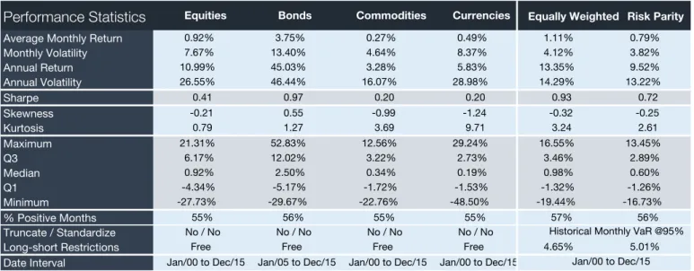
The out-of-sample results are tabulated in table 2 and pertain to the same period as the one considered in-sample. In equities, we obtain a sharpe ratio of 0.41. The annualized return and volatility are 10.99% and 26.55%, respectively. Although the return with expanding window estimates is almost double that of the in-sample result, the volatility also rises by more than half, yielding a sharpe ratio which is still close to the one obtained in-sample but slightly lower nonetheless. The skewness and kurtosis with this estimation procedure are similar to the values obtained in-sample, with kurtosis being actually smaller out-of-sample. In bond indices, we obtain a sharpe ratio of 0.97, which is close to the 1.06 figure obtained in-sample. The skewness and excess kurtosis statistics are also similar to the in-sample results. Therefore, our free model is robust where bond indices are concerned. In commodity indices, the model yields a sharpe ratio of 0.20, with a 3.28% annualized return, which is close to the 3.97% obtained in-sample. However, this return was achieved at the cost of higher volatility and left-tail returns, as seen by the more negative skewness and higher kurtosis, hence the drop in performance. In currencies, the out-of-sample sharpe ratio and annualized return are 0.20 and 5.83%, respectively. Although the annualized return is higher than in-sample, volatility and kurtosis likewise ramp up, likely due to the decrease in skewness which falls from 0.81 in-sample to -1.24 out-of-sample. Without future information, the model expectedly becomes more exposed to left-tail returns, with the lowest return recorded being -48.50% against the -11.91% observed in-sample.

(24)

The equally weighted portfolio and the risk-parity portfolio achieve a 0.93 and a 0.72 sharpe ratios out-of-sample, respectively. We have already identified the reason behind the equally weighted portfolio outperforming the risk-parity portfolio above. It is also worth mentioning the difference in historical VaRs using weighting scheme. The equally weighted portfolio generates a 4.65% 95% historical monthly VaR, while the risk-parity portfolio generates a higher VaR equal to 5.01%., despite its skewness and kurtosis being closer to zero than those of the equally weighted portfolio. The reason behind this is that this VaR overlooks some extremely negative returns recorded by the equally weighted portfolio, which the risk-parity succeeds in mitigating.

5.1.3. Year-to-Date Performance

After assessing how the strategy performed throughout the past two decades, the group considered interesting and enriching to evaluate its year-to-date out-of-sample performance; that is, the performance of the model from January 2016 through November 2016. It is important to underline that 2016 has shown to be an important, and tumultuous, year for financial markets, with several important events considerably shaping asset classes movements and respective performances throughout the year.

Table 3 reports the performance statistics for the period January 2016 to November 2016. In equities, we record a negative sharpe ratio of 0.09 due to an annualized return of -0.82%. The other models also generated negative sharpe ratios as we will discuss below. The cross-sectional average of equity indices returns over the period in question was 0.48%, driven by the poor performances of Italian Portuguese, Swiss, and Northern European equities which overshadowed emerging markets and British equities. The high value measures of Italian and Portuguese equity indices over 2016 suggest they were undervalued against the other equity indices in the sample. Despite their respective

(25)

momentum measures signalling that we should bet against these countries, the weight the model places on value is too high to yield non-positive weights during months when Italian and Portuguese equities severely underperformed. Although partly offset by other equity indices’ performance, such as British and emerging markets, the poor performance of Portuguese, Italian, Swiss, and Nordic equities underlie the negative sharpe ratio recorded. In bonds, we obtain a sharpe ratio of 1.15, on the back of an annualized return and volatility of 28.82% and 25.13%, respectively. The cross-sectional annualized average return over the period in question of the bond indices considered is 8.72%. Coupled with low volatilities, most indices yielded attractive sharpe ratios, being the cross-sectional average 0.75. Because we do not impose constraints on the amount of leverage we can employ, the model can take further advantage of the overall good performance of bond indices. Notice also the low skewness and excess kurtosis of the portfolio’s return. This means the model delivers good performance with low risk of left-tail events. In commodities, we achieve the highest sharpe ratio of the four asset classes, standing at 1.52. This result can be traced back to the overall good performance of commodity indices, with the cross-sectional annualized average return being 13.20% from January to November 2016. Although the 12.08% annualized return achieved by our portfolio seems low, especially when sectors such as energy and industry metals record 36.68% and 26.46% annualized returns over the same period, respectively, the annualized volatility of the commodity portfolio is only 7.97%. Given the high volatility of commodity indices (ranging from 14.55% to 28.91%, annualized), this risk-return trade-off obtained by our model is noteworthy. In currencies, we obtain a sharpe ratio of 1.05, with the annualized return and volatility being 6.40% and 6.13%. The cross-sectional annualized average return of currencies over 2016 was 3.91% and the most

(26)

volatile currency was the swiss frank with an annualized volatility of 11.9%. The performance achieved by the model can be traced back to the percentage of months in which the realized return was positive. During the 11-month period, the currency portfolio had eight months with positive returns, the highest recorded among the four asset classes. The equally weighted and risk-parity portfolios obtained sharpe ratios of 1.95 and 1.94, respectively. These are a result of the good performances of the bonds, commodities, and currencies portfolios, which combined, allow the investor to benefit from diversification gains as seen from the lower volatilities recorded (6.00% and 4.61% with the Equally Weighted and Risk-Parity approaches, respectively). The percentage of months with positive months is also illustrative of the positive effect diversification has on asset allocation, being it 82% and 73% in the equally weighted portfolio and risk-parity portfolio, respectively.

5.2. Long-only Model

As previously mentioned, the long only portfolio policy consists of a 100% investment in every asset class, i.e., no short positions are allowed neither on an asset class, nor in a single security and the total position on an asset class must be equal to 100%. Moreover, this model already accounts for transaction costs, assuming a constant cost per transaction of 25 basis points.

5.2.1. In-Sample Results

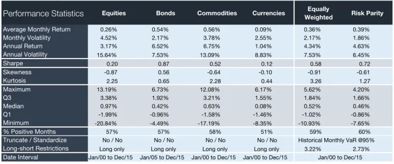
Starting with an individual comparison between asset classes, one can tell that the bond market continues to be the winner amongst all four classes in terms of return per risk as one can notice in Table 4. Under the in-sample analysis, this class yields an annual return of 6.53% and volatility of 7.53%, for a sharpe of 0.87, and an average monthly return of

(27)

0.54%. This performance corroborates what has been being described in our results: since the bond market has performed extraordinarily during the past years, a long position on this type of securities would most likely capture this outperformance. Also, it is important to highlight the narrow crash risk within this class, with skewness and kurtosis being equal to 0.56 and 0.65, respectively. In what concerns the worst performing class, Equities take the lead this time. Despite the average monthly return being positive and equal to 0.26%, its sharpe is poor and around 0.20 due to the enormous volatility observed. As we are analysing the past 15 years’ performance, we are incorporating serious macroeconomic events in our analysis that created significant market noise and thus, volatility peaks, such as the dotcom bubble, the sub-prime crisis and the government debt crisis, being the 2008 crisis the worst in terms of drawdown. Moreover, the long only model for equities performs the worst in-sample than any other model in terms of crash risk, reaching a kurtosis of 2.25, also the highest in this specific portfolio. The heavy tailed performance by the equity market is followed very closely by the Commodities market, with a similar kurtosis of 2.28. As for the return per unit of risk, commodities performed fairly better than Equities, achieving a sharpe of 0.52 mainly due to the higher return realised for lower levels of volatility. This strategy would yield positive returns for 58% of the months whereas for Currencies, this figure falls to 51%, the worst in this model, and the same can be said about its sharpe ratio of 0.12.

Allocating the assets under the equally weighted and risk parity scheme, one can notice the overall improvement of the model that potentially benefits from diversifying the portfolio with the four asset classes. In what concerns the first and second moments of the distribution, these are lower when compared with the free model, achieving sharpe figures of 0.58 and 0.72 for the equally weighted portfolio and the risk-rarity portfolio,

(28)

respectively. This is mostly due to the lower returns achieved which are not compensated enough by the lower volatilities to achieve sharpe ratios akin to those of the free model. We must recall that this model does include transaction costs, unlike the free model and thus, this decline in performance is expected and reasonable. Moreover, because weights cannot be negative nor levered, the long-only model can only attempt to exploit positive returns with lower funding ability. Therefore, returns should be considerably below those of the free model. Yet the performance achieved with the two portfolios under these two constraints is still satisfactory. Under the 15-year period analysed, the worst performances for the equally weighted and riskparity allocations were, respectively, 10.93% and -7.65%.

5.2.2. Out-Of-Sample Results

Not surprisingly, the performance winner is still the bonds class in terms of sharpe ratio; however, the worst performer by the same terms was currencies, with a sharpe ratio of 0.18 which is close to the one obtained in-sample. Nevertheless, all four asset classes record similar results to the ones previously obtained in-sample. The results for the out-of-sample analysis are tabulated in Table 5.

Apart from bond indices and currencies, the out-of-sample results of the long-only differ considerably from those of the free model. In equities, the sharpe ratio obtained is almost half of that achieved out-of-sample with the free model. This plunge in performance is likely tied to the negative impact of the non-negative weights and no leverage restrictions and transaction costs, which depress returns in too high a magnitude for the lower volatility to compensate and maintain a similar sharpe ratio to that in-sample. Surprisingly, however, the commodity portfolio in the long-only model continues to outperform its free model counterpart and achieves better results out-of-sample than

(29)

in-sample. This counterintuitive result is probably linked to the fact that the expanding window approach allows for coefficients to vary across time and thus pushing weights upward and seizing higher returns than the in-sample estimates. The latter, because is forward looking, may generate more conservative weights than out-of-sample as a precautionary measure for what lies ahead in time. Yet by looking at the worse second, third, and forth moments recorded in-sample, this conservative weights do not appear to pay off as there are bouts of negative returns for which they cannot adjust. Comparing the performance of the long-only commodity portfolio out-of-sample with that of free model, it seems that truncating the weights at zero is beneficial, likely due to the wrong signals given by the measures when they output negative weights. The number of months with positive returns with the long-only model is 2% higher than with the free model. When combining the four classes, we got satisfactory results in terms of Sharpe ratio for the equally weighted portfolio and the risk-parity portfolio, being them 0.62 and 0.76, respectively. In terms of cumulative returns, both portfolios performed decently during the period under analysis, obtaining a cumulative return at the end of 2015 equal to 133.98% under the EW allocation and 142.45% under the RP approach – Graph 4 in appendix. These statistics do not change significantly from those obtained in-sample, thereby showing the robustness of the long-only and transaction costs models. Although their performance was not as good as that of the free model, we refer once more to the explanation already provided when discussing the in-sample results.

5.2.3. Year-To-Date Results

As a way of assessing how the model would have performed during the former year and comparing it with the other two, a year-to-date analysis was performed for the Long Only model too.

(30)

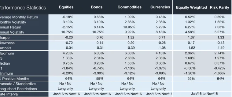
Like in the previous two models, despite the market turbulence of 2016, the Long Only portfolios also provided extraordinary results for Bonds, Commodities and Currencies, attaining Sharpe ratios of 0.76, 1.32 and 0.71, respectively. The downside risk was also considerably lower, with negative kurtosis figures being verified in the four asset classes. The best individual class performer was the Commodities class, mostly due to the long position early in the year in the precious metals and energy indices and due to the excellent returns during the month of November in the live cattle and industrial metals index, which aggregately provided an average monthly return of 1.09% for a 2.86% monthly volatility. The worst performer was the Equities class with a Sharpe ratio of -0.20, that on average, yielded -0.18% returns for the second highest monthly volatility, equal to 3.10%.

In aggregate terms, the diversification effect is again notorious, either in terms of the first two moments of the distribution, which were significantly better than the Semi-Restricted model, either in terms of downside risk. The EW and RP weighting schemes provided Sharpe ratios equal to 1.37 and 1.33, respectively, and Kurtosis figures equal to -1.52 and -1.19. The largest positive and negative monthly returns were achieved under the RP approach and were equal to 2.74% and -1.66%, respectively, and it also obtained the highest percentage of positive months, equal to 64%. It is important to bear in mind that although the RP allocation did not provide the best response to the 2016 macro events in terms of risk, it is likely that the information obtained during the former year will be incorporated to better manage possible future market turbulence.

Given the fact that these types of strategies are heavily historical and data dependent, the satisfactory results obtained are a strong signal that our model is robust while meeting the initial propositions.

(31)

6. Conclusion

We employ Brandt, Santa-Clara, and Valkanov (2009)’s parametric portfolio policy to build portfolios for equity indices, bond indices, commodity indices, and currencies based on the signals given by the value and momentum characteristics. Moreover, the flexibility of this model allows us to seamlessly incorporate the no-leverage and no-short-selling constraints imposed by Banco Invest into the model and build new portfolios which comply with said constraints. We can also account for transaction costs by implementing a model also proposed by the same authors, which not only enables us to include these costs in our analysis, but also allows for managing them. Subsequently, we combine these portfolios, built with (long-only) and without (free model) constraints, using two well-known cross-asset allocation approaches, the equal-weighting and risk-parity schemes. We obtain satisfactory results both in-sample and out-of-sample, even with constraints and transaction costs, thereby leading us to conclude that both models are to a high degree robust.

Focusing firstly on the unrestricted approach, our model achieved considerable benefits from the two exploited market anomalies, value and momentum, across the four considered classes of assets, while simultaneously limiting crash risk to adequate levels. After considering leverage and short-selling restrictions, which could potentially have an important impact in both in-sample and out-of-sample performance statistics, and consequently jeopardize the efficiency and attractiveness of the investment strategy, decent solutions were built and developed. The restricted long-only approach is the version of our model which is more likely applicable by Banco Invest, which, despite being heavily constrained, it still aims to best exploit momentum and value anomalies simultaneously, maximize investor’s utility. Notwithstanding a considerable slump in

(32)

annualized returns and sharpe ratios vis-à-vis the free model, the long-only model still provided strong results namely when considering the diversified-across-classes analysis. We consider that, in a world where it can be difficult to achieve relatively high investment returns, this developed investment strategy is a satisfactory alternative to capitalize attractive performance consistently, while not having to provide a subjective view on the markets and classes considered.

(33)

7. References

Alexander, Gordon J., and Alexandre M. Baptista. "Economic implications of using a mean-VaR model for portfolio selection: A comparison with mean-variance analysis." Journal of Economic Dynamics and Control 26.7 (2002): 1159-1193. Asness, Clifford S., Tobias J. Moskowitz, and Lasse Heje Pedersen. "Value and

momentum everywhere." The Journal of Finance 68.3 (2013): 929-985.

Barroso, Pedro, and Pedro Santa-Clara. "Beyond the carry trade: Optimal currency portfolios." Journal of Financial and Quantitative Analysis 50.05 (2015): 1037-1056. Baz, Jamil, et al. "Dissecting Investment Strategies in the Cross Section and Time

Series." Available at SSRN 2695101 (2015).

Blitz, David, and Pim Van Vliet. "Global tactical cross-asset allocation: applying value and momentum across asset classes." (2008).

Brandt, Michael W., Pedro Santa-Clara, and Rossen Valkanov. "Parametric portfolio policies: Exploiting characteristics in the cross-section of equity returns." Review of

Financial Studies 22.9 (2009): 3411-3447.

Burnside, Craig, Martin S. Eichenbaum, and Sergio Rebelo. Carry trade and momentum

in currency markets. No. w16942. National Bureau of Economic Research, 2011.

Carhart, Mark M. "On persistence in mutual fund performance." The Journal of

finance 52.1 (1997): 57-82.

Chaves, Denis B., et al. "What Drives the Value Premium? Risk versus Mispricing: Evidence from International Markets." Journal Of Investment Management (JOIM),

Fourth Quarter (2013).

Cooper, Ilan, Andreea Mitrache, and Richard Priestley. "A Global Macroeconomic Risk Explanation for Momentum and Value." Available at SSRN 2768040 (2016).

Fama, Eugene F., and Kenneth R. French. "Common risk factors in the returns on stocks and bonds." Journal of financial economics 33.1 (1993): 3-56.

Fama, Eugene F., and Kenneth R. French. "Multifactor explanations of asset pricing anomalies." The journal of finance 51.1 (1996): 55-84.

Haghani, Victor, and Richard Dewey. "A Case Study for Using Value and Momentum at the Asset Class Level." The Journal of Portfolio Management 42.3 (2016): 101-113. Jegadeesh, Narasimhan, and Sheridan Titman. "Momentum." (2001).

Jegadeesh, Narasimhan, and Sheridan Titman. "Returns to buying winners and selling losers: Implications for stock market efficiency." The Journal of finance 48.1 (1993): 65-91.

(34)

Korajczyk, Robert A., and Ronnie Sadka. "Are momentum profits robust to trading costs?." The Journal of Finance 59.3 (2004): 1039-1082.

Kroencke, Tim-Alexander, Felix Schindler, and Andreas Schrimpf. "International Diversification Benefits with Foreign Exchange Investment Styles CREATES Research Paper No. 2011-10." Available at SSRN (2011).

Ledoit, Olivier, and Michael Wolf. "Honey, I shrunk the sample covariance matrix." UPF

economics and business working paper 691 (2003).

Lustig, Hanno, N. Roussanov, and Adrien Verdelhan. Predictable currency risk premia. mimeo, 2009.

Markowitz, Harry. "Portfolio selection." The journal of finance 7.1 (1952): 77-91. Menkhoff, Lukas, et al. "Currency momentum strategies." Journal of Financial

Economics 106.3 (2012): 660-684.

Menkhoff, Lukas, et al. "Currency value." Available at SSRN 2282480 (2015).

Okunev, John, and Derek White. "Do momentum-based strategies still work in foreign currency markets?." Journal of Financial and Quantitative Analysis 38.02 (2003): 425-447.

Raza, Ahmad. "Are Value Strategies Profitable in the Foreign Exchange Market?." Available at SSRN 2559375 (2015).

Rouwenhorst, K. Geert. "International momentum strategies." The Journal of

Finance 53.1 (1998): 267-284.

Wang, Peng, and Larry Kochard. "Using a Z-score approach to combine value and momentum in tactical asset allocation." Available at SSRN 1726443 (2011).

(35)

8. Appendices

Table 1 – In-Sample Analysis, Free Model

Table 2 – Out-Of-Sample Analysis, Free Model

Free Model

In-sample analysis, Free Model

Performance Statistics Equities Bonds Commodities Currencies Equally Weighted Risk Parity

Average Monthly Return 0.50% 3.59% 0.33% 0.39% 0.98% 0.58%

Monthly Volatility 3.90% 11.71% 2.68% 3.58% 2.65% 2.18% Annual Return 6.00% 43.08% 3.97% 4.71% 11.78% 7.01% Annual Volatility 13.52% 40.57% 9.28% 12.39% 9.17% 7.54% Sharpe 0.44 1.06 0.43 0.38 1.28 0.93 Skewness -0.21 0.79 -0.71 0.81 0.12 -0.51 Kurtosis 1.23 1.33 1.02 5.16 1.71 0.83 Maximum 13.94% 43.18% 5.74% 18.05% 11.33% 5.10% Q3 2.86% 10.28% 2.14% 1.58% 2.64% 2.05% Median 0.48% 2.40% 0.49% 0.06% 1.23% 0.70% Q1 -1.73% -4.76% -1.28% -1.06% -0.93% -0.90% Minimum -12.11% -22.59% -9.46% -14.86% -7.31% -8.48% % Positive Months 57% 56% 57% 52% 66% 63% Truncate / Standardize No / No No / No No / No No / No

Long-short Restrictions Free Free Free Free 2.87% 2.89%

Date Interval Jan/00 to Dec/15 Jan/05 to Dec/15 Jan/00 to Dec/15 Jan/00 to Dec/15 Jan/00 to Dec/15 Historical Monthly VaR @95%

Expanding Window, Free Model

Monthly Volatility 7.67% 13.40% 4.64% 8.37% 4.12% 3.82% Annual Return 10.99% 45.03% 3.28% 5.83% 13.35% 9.52% Annual Volatility 26.55% 46.44% 16.07% 28.98% 14.29% 13.22% Sharpe 0.41 0.97 0.20 0.20 0.93 0.72 Skewness -0.21 0.55 -0.99 -1.24 -0.32 -0.25 Kurtosis 0.79 1.27 3.69 9.71 3.24 2.61 Maximum 21.31% 52.83% 12.56% 29.24% 16.55% 13.45% Q3 6.17% 12.02% 3.22% 2.73% 3.46% 2.89% Median 0.92% 2.50% 0.34% 0.19% 0.98% 0.60% Q1 -4.34% -5.17% -1.72% -1.53% -1.32% -1.26% Minimum -27.73% -29.67% -22.76% -48.50% -19.44% -16.73% % Positive Months 55% 56% 55% 55% 57% 56% Truncate / Standardize No / No No / No No / No No / No

Long-short Restrictions Free Free Free Free 4.65% 5.01%

Date Interval Jan/00 to Dec/15 Jan/05 to Dec/15 Jan/00 to Dec/15 Jan/00 to Dec/15 Jan/00 to Dec/15 Historical Monthly VaR @95%

(36)

Table 3 – Year-To-Date, Free Model

Table 4 – In-Sample Analysis, Long Only Performance 2016, Free Model

Performance Statistics Equities Bonds Commodities Currencies Equally

Weighted Risk Parity

Average Monthly Return -0.07% 2.40% 1.01% 0.53% 0.97% 0.75%

Monthly Volatility 2.69% 7.25% 2.30% 1.77% 1.73% 1.33% Annual Return -0.82% 28.82% 12.08% 6.40% 11.68% 8.96% Annual Volatility 9.31% 25.13% 7.97% 6.13% 6.00% 4.61% Sharpe -0.09 1.15 1.52 1.05 1.95 1.94 Skewness -0.78 0.45 0.67 -0.96 -0.88 0.17 Kurtosis 1.40 0.18 1.17 -0.08 2.12 -0.80 Maximum 3.77% 16.05% 5.92% 2.50% 3.80% 2.79% Q3 1.53% 5.56% 1.84% 1.70% 1.92% 1.70% Median -0.16% 2.37% 1.10% 1.17% 1.09% 0.53% Q1 -0.88% -2.35% -0.18% -0.20% 0.35% -0.19% Minimum -5.98% -9.50% -2.61% -2.73% -2.94% -1.42% % Positive Months 45% 55% 64% 73% 82% 73% Truncate / Standardize No / No No / No No / No No / No

Long-short Restrictions Free Free Free Free

Date Interval Jan/16 to Nov/16 Jan/16 to Nov/16 Jan/16 to Nov/16 Jan/16 to Nov/16 Jan/16 to Nov/16

Long only

In-sample analysis, Long only

Performance Statistics Equities Bonds Commodities Currencies _WeightedEqually Risk Parity

Long-short Restrictions Long only Long only Long only Long only 3.22% 2.73%

Date Interval Jan/00 to Dec/15 Jan/05 to Dec/15 Jan/00 to Dec/15 Jan/00 to Dec/15

Historical Monthly VaR @95%

(37)

Table 5 – Out-Of-Sample Analysis, Long Only

Table 6 – Year-To-Date, Long Only Performance 2016, Long Only

Average Monthly Return -0.18% 0.68% 1.09% 0.48% 0.52% 0.59%

Monthly Volatility 3.10% 3.10% 2.86% 2.36% 1.32% 1.52% Annual Return -2.15% 8.14% 13.05% 5.79% 6.27% 7.03% Annual Volatility 10.75% 10.75% 9.92% 8.18% 4.58% 5.27% Sharpe -0.20 0.76 1.32 0.71 1.37 1.33 Skewness -0.72 0.14 0.20 -0.26 0.17 -0.13 Kurtosis -0.04 -0.31 -0.39 -1.08 -1.52 -1.19 Maximum 4.20% 6.06% 6.38% 4.13% 2.36% 2.74% Q3 1.33% 2.34% 2.68% 2.06% 1.60% 1.97% Median 0.75% 0.28% 1.53% 0.86% 0.67% 0.57% Q1 -1.84% -0.74% -1.13% -1.37% -0.50% -0.42% Minimum -6.20% -3.90% -3.12% -3.09% -1.20% -1.66% % Positive Months 64% 55% 64% 64% 55% 64% Truncate / Standardize No / No No / No No / No No / No

Long-short Restrictions Long only Long only Long only Long only

Date Interval Jan/16 to Nov/16 Jan/16 to Nov/16 Jan/16 to Nov/16 Jan/16 to Nov/16 Jan/16 to Nov/16

Expanding Window, Long only

Performance Statistics Equities Bonds Commodities Currencies _WeightedEqually Risk Parity

Long-short Restrictions Long only Long only Long only Long only 3.47% 2.68%

Date Interval Jan/00 to Dec/15 Jan/05 to Dec/15 Jan/00 to Dec/15 Jan/00 to Dec/15

Historical Monthly VaR @95%

(38)

Graph 1 – In-Sample Cumulative Return, Free Model

Graph 2 – Out-Of-Sample Cumulative Return, Free Model

-100% 0% 100% 200% 300% 400% 500% 600% 2000 2001 2002 2003 2004 2005 2006 2007 2008 2009 2010 2011 2012 2013 2014 2015 Cu m ul at iv e Re tu rn Cumulative Return Equally Weighted Risk Parity -100% 0% 100% 200% 300% 400% 500% 600% 700% 800% 900% 2000 2001 2002 2003 2004 2005 2006 2007 2008 2009 2010 2011 2012 2013 2014 2015 Cu m ul at iv e Re tu rn Cumulative Return Equally Weighted Risk Parity

(39)

Graph 3 – In-Sample Cumulative Return, Long Only

Graph 4 – Out-Of-Sample Cumulative Return, Long Only

-40% -20% 0% 20% 40% 60% 80% 100% 120% 140% 160% 180% 2000 2001 2002 2003 2004 2005 2006 2007 2008 2009 2010 2011 2012 2013 2014 2015 Cu m ul at iv e Re tu rn Cumulative Return Equally Weighted Risk Parity -50% 0% 50% 100% 150% 200% 2000 2001 2002 2003 2004 2005 2006 2007 2008 2009 2010 2011 2012 2013 2014 2015 Cu m ul at iv e Re tu rn Cumulative Return Equally Weighted Risk Parity