Research Article Geospatial Analysis of Extreme Weather Events in Nigeria (1985–2015) Using Self-Organizing Maps

(1)

Research Article

Geospatial Analysis of Extreme Weather Events in

Nigeria (1985–2015) Using Self-Organizing Maps

Adeoluwa Akande,

1

Ana Cristina Costa,

1

Jorge Mateu,

2

and Roberto Henriques

1

1_{NOVA IMS, Universidade Nova de Lisboa, Campus de Campolide, 1070-312 Lisboa, Portugal} 2_{Department of Mathematics, Universitat Jaume I, 12071 Castellon, Spain}

Correspondence should be addressed to Adeoluwa Akande; akandeadeoluwa@gmail.com

Received 18 January 2017; Revised 29 June 2017; Accepted 9 July 2017; Published 9 August 2017

Academic Editor: Efthymios I. Nikolopoulos

Copyright © 2017 Adeoluwa Akande et al. This is an open access article distributed under the Creative Commons Attribution License, which permits unrestricted use, distribution, and reproduction in any medium, provided the original work is properly cited.

The explosion of data in the information age has provided an opportunity to explore the possibility of characterizing the climate patterns using data mining techniques. Nigeria has a unique tropical climate with two precipitation regimes: low precipitation in the north leading to aridity and desertification and high precipitation in parts of the southwest and southeast leading to large scale flooding. In this research, four indices have been used to characterize the intensity, frequency, and amount of rainfall over Nigeria. A type of Artificial Neural Network called the self-organizing map has been used to reduce the multiplicity of dimensions and produce four unique zones characterizing extreme precipitation conditions in Nigeria. This approach allowed for the assessment of spatial and temporal patterns in extreme precipitation in the last three decades. Precipitation properties in each cluster are discussed. The cluster closest to the Atlantic has high values of precipitation intensity, frequency, and duration, whereas the cluster closest to the Sahara Desert has low values. A significant increasing trend has been observed in the frequency of rainy days at the center of the northern region of Nigeria.

1. Introduction

One of the visible impacts of climate change and climate variability is extreme weather events that occur from time to time in several parts of the globe. A climate extreme is “the occurrence of a value of a weather or climate variable above (or below) a threshold value near the upper (or lower) ends of the range of observed values of the variable” [1]. Climate extremes can result in changes in the frequency, intensity, spatial extent, duration, and timing of climatic phenomena. There is a growing global concern that anthropogenic activ-ities are a major cause of the variability in the intensity and frequency of weather and climate extremes [2–4]. However, it can also be argued that climate extremes are just a part of decadal global climate cycle and variability [5].

Climate extremes, including the ones related to precipi-tation, can be analyzed using several approaches [6–8]. The use of indices to characterize the frequency, intensity, and duration of precipitation extremes is one of the ways to assess them [9–12]. The joint working group CCI/CLIVAR/JCOMM

Expert Team on Climate Change Detection and Indices (ETCCDI) (http://etccdi.pacificclimate.org/index.shtml) has 27 standardized and recommended climate extreme indices [2, 13–15]. This set of indices includes both temperature and precipitation indices.

Precipitation is one of the most important climatic parameters responsible for flood and drought in several vulnerable parts of the world. According to [1], there is a high chance that the frequency of heavy precipitation and total precipitation will increase in several parts of the globe in the 21st century. Evidence of climate change in Nigeria has been discussed by [16], who reported increasing damage caused by wind and rainstorms, which are projected to increase in southern regions [17]. The northern part of the country has been experiencing a reduction in rainfall and an increase in the rates of dryness and heat [18, 19], while the rainfall amounts have been increasing in the southern part with an irregular pattern [19, 20]. Moreover, climate projections for the 21st century show a significant increase of temperature over all the ecological zones [17] which may have negative

(2)

impacts on agriculture and food security. Reference [21] evaluated how crop yield might respond to climate change in Nigeria, and [22] discussed the challenges of agricultural adaptation to climate change.

Proper study of climate extremes depends on the quality and quantity of data, as well as on how rigorously they are analyzed [1]. When dealing with precipitation extremes, it is important to consider their synoptic aspects and dimen-sions. The recent increase of data from ground observations, satellites, and numerical models enables the opportunity for exploring the use of data mining techniques in climatic stud-ies [6]. One of such techniques is Cluster Analysis (CA). The use of CA to gain insight from geographical data had more serious adoption since the 1990s [23]. Several attempts have been made in the past to characterize extreme climate using machine learning methods. Self-Organizing Maps (SOM) have successfully been applied to several climate research including the analysis of atmospheric circulations variability [24], time evolution of seasonal climate [25], and climate model downscaling [26] and to access the stationary of global climate models [27].

Reference [28] did a study on the spatial and tem-poral variation of extreme weather in the Iberian Penin-sula using seven different temperature and precipitation indices. Using geostatistics, these indices were analyzed and Inverse Distance Weighting (IDW) maps were produced to compare the spatial and temporal surface distribution of the indices. Clustering was thereafter done using SOM to study areas with similar climatic characteristics for two time periods, 1951–1980 and 1981–2010. The SOM analysis was done separately for temperature and precipitation indices as mixing both indices together did not provide consistent conclusions in the Iberian Peninsula. Reference [6] also visualized extreme climate conditions using linear models (ordinary kriging and ordinary cokriging) and a nonlinear model (a three-dimensional SOM). They made use of indices calculated from precipitation data obtained between 1998 and 2000 from nineteen meteorological station covering Madeira Island in Portugal.

Nigeria has had its fair share of climate extremes in recent times. The floods of July 10, 2011, in Lagos, August 26, 2011, in Ibadan and more recently nationwide floods of 2012 are all pointers to the extreme precipitation being experienced in the country [29]. In Nigeria, making use of nine indices, the authors [30] were able to study climate extremes over Kano making use of temperature and precipitation data. Using temperature data, the authors could notice a warming trend characterized by an increase in the number of warm days and warm spell. The rainfall data showed a similar increase in the amount of rainfall over the region. Other studies have attempted to use linear approaches to study temperature and rainfall trends over various parts of the country [31– 33]. However, none of these studies have attempted to study their spatial local patterns. A first attempt to use data mining techniques in climatic studies of Nigeria was carried out by [34]. Making use of a Time Lagged Feedforward Network (TFLN) and recurrent network, they could predict the future values of 8 climatic parameters.

This study will however be focused on the geoexploration of climate extremes as opposed to its prediction. Based on the framework proposed by [6], this research will be making use of a SOM to visualize the phenomenon from a global perspective.

The atmosphere is a continuum and SOM aids the visu-alization of this continuum by placing very different atmo-spheric states on distant nodes and similar atmoatmo-spheric states on adjacent nodes. Using a two-dimensional sheet, SOM (the default SOM shape) creates 4 vertices and hence produces an edge effect [35], which can be solved with the cylinder and toroidal shapes which also provide a continuous surface [36]. The objective of this research is to cluster precipita-tion extreme over Nigeria, characterize regions of similar precipitation patterns, and characterize its evolution over a period of 31 years. Our study area is first introduced with emphasis on its climate to give a background on the type of climate we are working with. CHIRPS dataset is subsequently introduced as the precipitation data from which precipitation extreme indices are calculated. The methodology used for this research is explained and results obtained are laid out. We wrap up this paper with a conclusion.

2. Materials and Methods

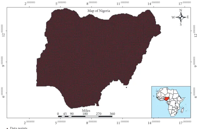
2.1. Study Area. Nigeria is a country located in West Africa. It

lies between 4∘N and 14∘N latitude and 4∘E and 14∘E longitude

and is bordered in the South by the Atlantic Ocean and the North by the Sahara Desert (Figure 1). This gives the country a very wide range of climatic pattern experienced throughout the year.

Its weather system is controlled by the Intertropical Discontinuity (ITD). The ITD is the area of lowest pressure over West Africa separating the moist Southwest Monsoon from the Atlantic Ocean and the dry northeast trade winds from the Sahara Desert. Hence, the ITD can be located with the aid of a change in wind direction as well as the amount of moisture in the atmosphere. This is also given by the dew point temperature. The south of the ITD usually has a dew

point temperature greater than 15∘C while the north of the

ITD usually has a dew point temperature lower than 15∘C. The

atmosphere to the south of the ITD is usually moist aiding the formation of clouds at low altitude including fog while the atmosphere to the north of the ITD is usually dry and dusty preventing the formation of clouds except altocumulus and cirrus at high level [37–39].

The movement of the ITD controls the weather systems in Nigeria. It has three unique overlapping movements through-out the year, an annual movement which follows the path of the sun and is responsible for seasons, a diurnal movement consisting of a slight southward shift in the morning and a slight northward shift in the afternoon, and intermediate movements observed during the northern hemisphere winter months [37].

(3)

0 45 90 180 270 360

12

.000000

9

.000000

6

.000000

Data points

Miles

Map of Nigeria N

W E S

2.000000 5.000000 8.000000 11.000000 14.000000 17.000000

12

.000000

9

.000000

6

.000000

Figure 1: Study area in Nigeria with data points.

the southwest. The main ecological zones in Nigeria are the tropical rainforest in the south, savannah in the middle belt, and semiarid zones in the north.

2.2. Data. A set of high resolution reanalysis climatic daily data from the Climate Hazards Group Infrared Precipita-tion with StaPrecipita-tions (CHIRPS) from 1985 to 2015 covering our study area will be used (ftp://chg-ftpout.geog.ucsb.edu/ pub/org/chg/products/CHIRPS-2.0/). CHIRPS is a

quasig-lobal (50∘S–50∘N) satellite and observation based

precipi-tation estimates over land. It is a 0.05-degree resolution (about 5.5 kilometres) gridded dataset [41]. Reanalysis data, unlike conventional data, provides a more wholesome look at global climatic circulation and can be used as an alternative to ground observation data [42]. The data comes in the Network Common Data Form (NetCDF) format and will be manipulated using Matlab, Microsoft Excel, and ArcGIS software. The Network Common Data Form (NetCDF) is a file format for storing multidimensional scientific data (variables) such as temperature, humidity, and rainfall. The CHIRPS reanalysis data has specifically been validated for the monitoring of climatic extremes with good performance. This data was obtained online from the Climate Hazards Group InfraRed Precipitation with Station data (CHIRPS) (ftp:// chg-ftpout.geog.ucsb.edu/pub/org/chg/products/CHIRPS-2.0/; accessed: September, 2016). For details, see [43].

This research utilized four of the precipitation indices as defined by ETCCDI (Table 1). This is because each of the indices, by itself, shows only a part of the problem [13, 14]. The four selected are able to achieve a holistic characterization

of precipitation in its different perspectives [6]. By holistic characterization, we are referring to their ability to capture changes in amount, frequency, and intensity.

2.2.1. Data Preparation and Preprocessing. The representation and quality of data are very important in determining the quality of clusters that will be seen [44]. Hence, there is a need to do some amount of preprocessing to the data before clustering. Given that we are making use of a gridded reanalysis data, we expect to have a consistent and coherent data without outliers or missing values. For this research, several data preparatory tasks were carried out prior to actual analysis, including the following:

(i)Dimensionality Reduction. Out of the several temper-ature and precipitation indices defined by ETCCDI to characterize climate extremes, four precipitation indices (Table 1) were selected based on previous studies by [6] and expert opinion to characterize the duration, intensity, and frequency of precipitation over our study area.

(ii)Data Extraction. Matlab was used to calculate the four indices and extract them into Microsoft Excel

tables for each year. ArcMapwas further used to clip

out our area of interest (Nigeria) from the extracted dataset and export them back to Microsoft Excel for exploratory data analysis

(iii)Data Normalization. This is the scaling down of the

(4)

Table 1: Summary of rainfall indices used in the study (a wet day is defined as a day with at least 1 mm of precipitation).

Index Descriptive name Definition Units

R1 Number of wet days Frequency of rainy days Days

R×1d Maximum 1-day precipitation Maximum 1-day precipitation mm SDII Simple daily intensity index Ratio between the total rain on wet days

and the number of wet days mm/day

R×5d Maximum 5-day precipitation Highest consecutive 5-day precipitation mm

it if that is the aim), thus enabling the data analysis method to treat the data “fairly” [45]. Normalizing the data will help to standardize the scale effect each variable has on the final results. To achieve this, each index was standardized using its minimum and maximum values. This way, we ensured that the values of each variable range between 0 and 1.

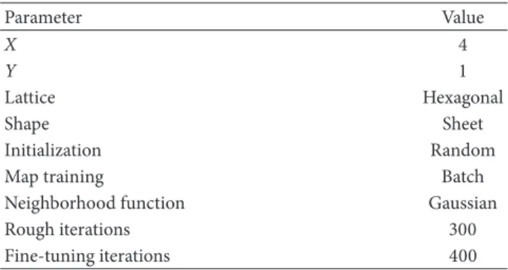
2.3. Methodology. SOM are nonsupervised neural networks used for clustering, dimension reduction, and visualization. This research aims to achieve these three objectives by visually showing the areas with similar precipitation extreme characteristics using the indices outlined before. SOM can map high-dimensional data onto one or two dimensions while maintaining the topology of the data structure. [46]. SOM works by mapping an n-dimensional data space onto a grid of neurons. These grids of neurons are usually in a two-dimensional data space and rectangular. During training, the Euclidean distance between a neuron and all units in the data space is calculated and the closest is selected. This is called the Best Matching Unit (BMU). This process is iterated and a parameter called the learning rate is used to ensure that the training converges. Although, no preference is given to the spatial property of our climatic data, spatial autocorrelation makes it possible for the BMU attached to each neuron to be geographically close thereby creating clusters that are geographically together. Compared to other clustering methods, Self-Organizing Maps (SOM) are robust even in the presence of outliers and results easier to understand and interpret. They also have very good visualization tools like the GeoSOM suite [47]. This algorithm has been implemented in a GeoSOM suite based on the SOM toolbox in Matlab and is used for clustering the climatic data. The dataset is trained and modelled using the SOM algorithm, producing several views and interactively exploring the data, hoping to gain valuable insights. Several parameters were used to initialize the SOM to obtain different models for each year and the final parameters used are given in Table 2. The model with the least quantization error was chosen as the best fit [48].

For this research, GeoSOM was also used to detect out-liers, for sensitivity analysis of the parameters of the methods used, for the analysis of the U-matrix, and for component planes and for the final clustering. After removing the

outliers, a new 4×1 SOM was trained using the parameters

in Table 2.

After clustering, the index values of the centroid of each cluster are calculated and their trend is analyzed through time. The Mann-Kendall test is used to verify if those index values exhibit a monotonic trend. The Mann-Kendall statistic

Table 2: Values of the parameters used to implement the GeoSOM algorithm.

Parameter Value

X 4

Y 1

Lattice Hexagonal

Shape Sheet

Initialization Random

Map training Batch

Neighborhood function Gaussian

Rough iterations 300

Fine-tuning iterations 400

is calculated as follows. Let S be the number of positive

differences minus the number of negative differences between data values:

𝑆 =𝑛−1∑

𝑗=1 𝑛

∑

𝑘=𝑗+1

sgn(𝑥_𝑘− 𝑥_𝑗) , (1)

where 𝑥_𝑘 and 𝑥_𝑗 are data values,𝑛is the number of years

under study, and sgn is an indicator function that takes on

the values 1, 0, or−1 according to the sign of𝑥_𝑘− 𝑥_𝑗.

A positive (negative) value of𝑆 indicates an increasing

(decreasing) trend. 𝑆is normally distributed [49, 50] with

variance given by

𝑉 (𝑆) = 118 (𝑛(𝑛 − 1)(2𝑛 + 5)). (2)

The test statistic𝑍_𝑠is given by

𝑍𝑠=

{ { { { { { { { { { { { {

𝑠 − 1

√𝑉 (𝑆) for𝑆 > 0

0 for𝑆 = 0

𝑠 + 1

√𝑉 (𝑆) for𝑆 < 0.

(3)

The significance of the trend can be verified by comparing

the observed value of𝑍_𝑠with the appropriate percentiles of

(5)

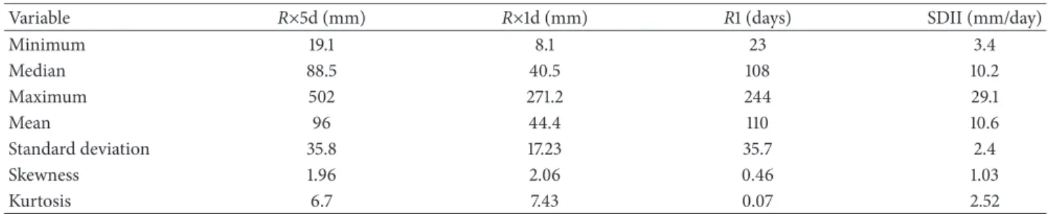
Table 3: Summary statistics of the precipitation indices for the period 1985–2015.

Variable R×5d (mm) R×1d (mm) R1 (days) SDII (mm/day)

Minimum 19.1 8.1 23 3.4

Median 88.5 40.5 108 10.2

Maximum 502 271.2 244 29.1

Mean 96 44.4 110 10.6

Standard deviation 35.8 17.23 35.7 2.4

Skewness 1.96 2.06 0.46 1.03

Kurtosis 6.7 7.43 0.07 2.52

Table 4: Correlation matrix of the precipitation indices for the period 1985–2015 (significant at 5% level).

Longitude Latitude R×5d R1 R×1d SDII

Longitude 1

Latitude 0.253906 1

R×5d −0.13109 −0.72777 1

R1 −0.33055 −0.91357 0.749444 1

R×1d −0.27179 −0.58645 0.753508 0.579652 1

SDII −0.19219 −0.80291 0.838971 0.736548 0.714564 1

3. Results and Discussion

3.1. Exploratory Analysis. A total of 30155 equally spaced points spread over Nigeria were analyzed for each year. Des-criptive statistics were computed for each of the four indices for each year as well as collectively for the entire period under study (Table 3). With Nigeria being sandwiched between the moist Atlantic Ocean and the dry Sahara Desert in the tropics, Table 3 shows the huge climatic disparity in Nigeria with some parts of Northern Nigeria having only 23 wet days in a year while some areas in the south have as much as 244 wet days out of 365 days in a year. Also, some areas have a maximum one day precipitation of 8.1 mm while other areas have a maximum one day precipitation of 271.2 mm. Scatter-plots (not shown) of the indices for each year provide evidence of a strong positive linear relationship between all indices. This linear relationship was summarized using the

correlation coefficient (Table 4). The𝑝values of the

corre-lation coefficient are all less than the significance level (0.05) and hence, there is significant evidence to conclude that there is a significant linear relationship between the indices. There-fore, we can conclude that all indices are moderately corre-lated, thus indicating their suitability to characterize the dif-ferent features of the precipitation regimes in Nigeria [6]. This means that all four indices are moderately interconnected and where we have a very high maximum 5-day precipitation, for example, we will also most likely have a high precipitation intensity and vice versa.

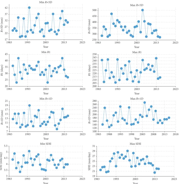
The temporal variation of the mean index values was also investigated (Figure 2) and shows that 2006 had both the

highest mean consecutive 5-day precipitation (R×5d index)

averaged over our entire study area with a value of 112.2 mm and the maximum highest consecutive 5-day precipita-tion with a value of 502 mm. However, a minimum highest consecutive 5-day precipitation occurred in 1989 with a value of 19.1 mm. 2013 had the highest number of wet days with 244

days having rainfall greater than 1 mm (R1 index), while 1987

had just 23 wet days being the driest in our study period. The highest average intensity of rainfall in a raining day (SDII) was recorded in 1999 as 29.1 mm/day, while the low-est average rainfall intensity was recorded in 1989 as 3.4 mm/ day. Furthermore, the highest maximum 1-day precipitation

(R×1d index) of 271.2 mm was observed in 2004, and the

minimum was 8.1 mm in 2009.

Histograms (not shown) were also plotted for each index by year to check for moderate and heavy extreme values which could be typical values, outliers, or perhaps errors. It also helped to graphically perceive the distribution frequency of the indices. Some years exhibit a “bell-shaped” curve in the histograms, but the majority shows a positively skewed distribution.

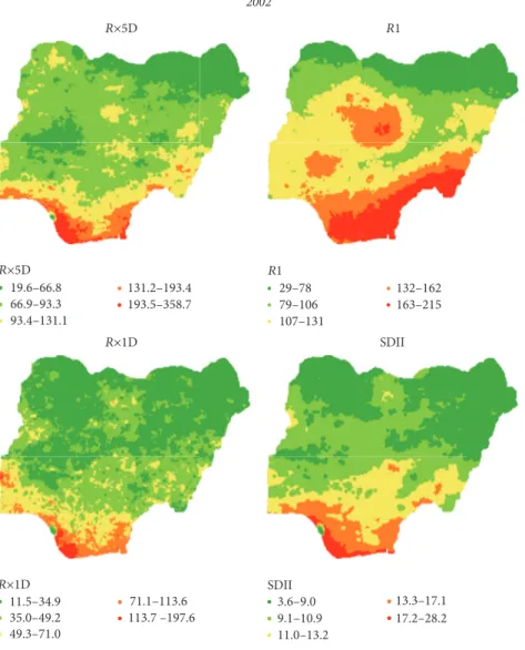
The previous analyses are based on averaged values over the entire study region, thus they are not reflective of the unique precipitation property of specific regions. Nigeria has a broad range of precipitation extremes in various regions. Hence, further analyses were conducted to explore and characterize each region. Exploratory spatial data analysis was used to detect spatial patterns and formulate hypothesis based on the geography of the data. From the posting of the data points (Figure 3) it is clear that the spatial resolution of the dataset is so high (approximately 5.5 km) that maps look like interpolated surfaces. Hence, there is no need to interpolate the data points to a surface using a linear model (e.g., ordinary kriging or cokriging). The overall trend in the study region corresponds to decreasing values from the southern part of Nigeria to the north in all indices. However, each index shows a unique pattern of variation (Figure 3).

3.2. GeoSOM Results

(6)

Min

17 22 27 32 37 42

1993 2003 2013 2023 1983

Year

Max

1993 2003 2013 2023 1983

Year 250

300 350 400 450 500

Max R₁

200 205 210 215 220 225 230 235 240 245 250

R

1 (da

ys)

1993 2003 2013 2023 1983

Year Min R₁

20 25 30 35 40 45

R

1 (da

ys)

1993 2003 2013 2023 1983

Year Min

7 9 11 13 15 17 19 21

1993 2003 2013 2023 1983

Year

Max

1988 1993 1998 2003 2008 2013 2018 1983

Year 100

120 140 160 180 200 220 240 260 280

Max SDII

19 21 23 25 27 29 31

SD

II (mm/da

y)

1993 2003 2013 2023 1983

Year Min SDII

1993 2003 2013 2023 1983

Year 3

3.5 4 4.5 5 5.5

SD

II (mm/da

y)

R×5_D

R×1_D

R×5

D (mm)

R×5

D (mm)

R×1

D (mm)

R×1

D (mm)

R×1_D

Figure 2: Temporal variation of mean index values over Nigeria from 1985 to 2015.

were subsequently identified by searching for very high values in a U-matrix. A U-matrix is a visual representation of a self-organizing map (SOM) where the Euclidean distance between neurons is represented in a colour-coded image. If represented as an image with colours ranging from blue to red, then lighter shades of blue will indicate closely spaced neurons while darker shades of blue will indicate distant neurons. Therefore, a group of light colours (blue) can be regarded as a cluster and the dark colours (blue) regarded as boundaries of the cluster. From our analysis, outliers can be clearly identified as bright red spots at the upper left

(7)

2002

R1

SDII 19.6–66.8

66.9–93.3 93.4–131.1

131.2–193.4 193.5–358.7

R1

29–78 79–106 107–131

132–162 163–215

11.5–34.9 35.0–49.2 49.3–71.0

71.1–113.6 113.7 –197.6

SDII 3.6–9.0 9.1–10.9 11.0–13.2

13.3–17.1 17.2–28.2

R×1_D

R×5_D

Figure 3: Data posting of indices values from 2002.

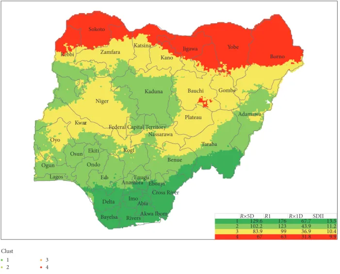
3.2.2. Spatial Trends. A 4 × 1 SOM was used because we wanted to obtain 4 clusters which is in line with number of Koppen climate classification zones over Nigeria. As expected, there is evidence of spatial autocorrelation in the pattern of the clusters (Figure 5). Four regions with similar precipitation characteristics are evident varying from the south to the north through the middle belt of Nigeria. Although these clusters bare some resemblance with the Koppen climatic zones, there are still several variations in the spatial extent of each zone when both are compared. However, this is not surprising since the Koppen classification characterizes mean climatic characteristics, and the clusters are based on extreme precipitation indices. For better clarity in interpretation, we have applied a colour scheme to the value of each precipitation index in a tabular form so that we can easily identify the colour’s that represent high (red), mean (yellow), and low (green) values of each index. The table in Figure 5 shows the mean value of each index in a cluster.

Cluster 1 covers the Niger-Delta and southeast region of the country. It is characterized by very high precipitation amount, intensity, and frequency. This is because of the

southwestern trade winds that bring a lot of moisture inland from the Atlantic Ocean in the south. Because of the high moisture, this region experiences heavy and abundant mon-soonal rainfall and is cloudy all year round. Hence, they have a typical tropical monsoon climate.

Cluster 2 covers the southwest and extends further inland. Although not as high as cluster 1, it is also characterized by high intensity, frequency, and amount of rainfall. This region experiences two peaks of rainfall in a year with a little dry season in August. The first rainfall peak is usually characterized by thunderstorms and occurs in June, while the second rainfall peak is usually monsoonal and occurs around September. A portion of this cluster appears as an island in the middle belt around Jos, Kaduna and Abuja, surrounded by cluster 3. This might be explained by the terrain of this region, which is a plateau with high elevation. Hence, it has a semitemperate climate. Therefore, it is interesting to note that it bears similar precipitation characteristics with south-western Nigeria.

(8)

(a)

sdiin

r1n

0 0.2 0.4

V

al

ues

0.6 0.8 1

n

r×5_d r×1_dn

(b)

Sel

Normal values Outliers

(c)

Figure 4: U-matrix (a), boxplot (b), and map (c) of the four precipitation indices showing outliers in red in 2003.

rainfall during the raining season. Rainfall in this region is primarily associated with thunderstorms and high wind gusts. This is the region where the south-westerlies meet the north-easterlies to create what is known as the Intertropical Discontinuity (ITD). The ITD is a region of low pressure and an important factor for Nigeria weather and climate [51].

Cluster 4 is located predominantly in the northern part of the country. This is a dry and dusty area with the North-Easterly trade winds bringing in dry and dusty air masses from the Sahara Desert. Results show that this region experiences minimal rainfall in terms of amount, duration, frequency, and intensity (see table in Figure 5). The raining season in this region is very short lasting just about three months.

3.2.3. Temporal Trends. There was a tendency for the maxi-mum 1-day precipitation, maximaxi-mum 5-day precipitation, and frequency of rainy days to increase with time in clusters 1, 2, and 4. This result is consistent with previous study done in Kano State, Nigeria, which showed an increase in maximum 5-day precipitation with time [30]. In contrast, the maximum 1-day precipitation decreases with time in cluster 3. The intensity of rainfall was constant in cluster 1 throughout the period under study, while a decreasing trend is noticed in rainfall intensity and maximum 1-day precipitation in cluster

3. However, considering the results of the Mann-Kendall test, those trends were not significant (Figure 6). The only sta-tistically significant upward trend is noticed in the frequency of rainy days in cluster 4. These results are not different from that obtained and reported globally in some regions of the world [52]. Specially in the tropics, the intensity of preci-pitation extremes is expected to increase with a warming climate [53].

4. Conclusion

(9)

Niger

Borno Yobe

Taraba Bauchi

Oyo Kebbi

Kaduna

Kogi Kwara

Benue

Edo Zamfara Sokoto

Adamawa Plateau

Kano

Jigawa Katsina

Delta Ogun Ondo

Gombe

Nassarawa

Osun

Rivers Imo Ekiti

Enugu

Bayelsa

Ebonyi Lagos

Cross River Abia

Akwa Ibom Anambra

Federal Capital Territory

Clust 1 2

3 4

R1 _SDII

1 129.6 176 67.7 13.5 2 102.2 123 43.9 11.2 3 83.9 99 36.9 10.4 4 67 63 31.8 9.9

R×1_D R×5_D

Figure 5: Precipitation indices clustering over Nigeria in 2003.

ZS

Critical values ( = 5_%)

RX

5

D_

1

R

1

_

1

RX

1

D_

1

SD

II_

1

RX

5

D_

2

R

1

_

2

RX

1

D_

2

SD

II_

2

RX

5

D_

3

R

1

_

3

RX

1

D_

3

SD

II_

3

RX

5

D_

4

R

1

_

4

RX

1

D_

4

SD

II_

4

−_2.5 −₂ −_1.5 −₁ −_0.5

0 0.5 1 1.5 2 2.5

Figure 6: Observed values of Mann-Kendall’s test statistic ZS.

agricultural practices will be important in determining future crop yields in the region.

We have been able to identify the spatial and temporal patterns of extreme precipitation and thus gain valuable insights into the spatial and temporal dynamics of precip-itation in Nigeria. However, the temporal resolution of the dataset is too small to adequately characterize the long-term behavior of extreme precipitation in Nigeria. Further research with a higher temporal resolution dataset should be pursued.

Conflicts of Interest

The authors declare that there are no conflicts of interest regarding the publication of this paper.

Acknowledgments

(10)

IMS), Department of Geoinformatics at the University of Munster and Universitat Jaume I.

References

[1] IPCC,Managing the Risks of Extreme Events And Disasters to Advance Climate Change Adaptation, 2012.

[2] A. M. G. K. Tank, F. W. Zwiers, and X. Zhang, “Guidelines on Analysis of extremes in a changing climate in support of informed decisions for adaptation,” Climate Data and Mon-itoring, vol. 52, WCDMP-No. 72, 2009, Retrieved from File Attachment.

[3] IPCC,Climate Change 2007: The Physical Science Basis. Contri-bution of Working Group I to the Fourth Assessment Report of the Intergovernmental Panel on Climate Change, Cambridge University Press, Cambridge, United Kingdom and New York, NY, USA, 2007, Retrieved from papers3://publication/uuid/ 789C871F-F7F3-4AD1-A26B-017707E6A214.

[4] R. Stefan, “Anthropogenic climate change: revisiting the facts,”

History, vol. 140, no. 6, pp. 34–53, 2005.

[5] IPCC, Climate Change 2014: IPCC Fifth Assessment Synthe-sis Report-Summary for Policymakers-an Assessment of Inter-Governmental Panel on Climate Change, Cambridge University Press, Cambridge, UK, 2014.

[6] J. Gorricha, V. Lobo, and A. C. Costa, “A Framework for Exploratory Analysis of Extreme Weather Events Using Geosta-tistical Procedures and 3D Self-Organizing Maps,”International Journal on Advances in Intelligent Systems, pp. 16–26, 2013, http://citeseerx.ist.psu.edu/viewdoc/download.

[7] M. R. Jones, S. Blenkinsop, H. J. Fowler, and C. G. Kilsby, “Objective classification of extreme rainfall regions for the UK and updated estimates of trends in regional extreme rainfall,”

International Journal of Climatology, vol. 34, no. 3, pp. 751–765, 2014.

[8] E. Thibaud, R. Mutzner, and A. C. Davison, “Threshold mod-eling of extreme spatial rainfall,”Water Resources Research, vol. 49, no. 8, pp. 4633–4644, 2013.

[9] L. V. Alexander, X. Zhang, T. C. Peterson et al., “Global observed changes in daily climate extremes of temperature and precipita-tion,”Journal of Geophysical Research D: Atmospheres (1984– 2012), vol. 111, no. D5, 2006.

[10] M. G. Donat, L. V. Alexander, H. Yang et al., “Updated analyses of temperature and precipitation extreme indices since the beginning of the twentieth century: the HadEX2 dataset,”

Journal of Geophysical Research D: Atmospheres, vol. 118, no. 5, pp. 2098–2118, 2013.

[11] A. Moberg, P. D. Jones, D. Lister et al., “Indices for daily temperature and precipitation extremes in Europe analyzed for the period 1901–2000,”Journal of Geophysical Research Atmos-pheres, vol. 111, no. 22, 2006.

[12] E. J. M. Van den Besselaar, “Trends in European precipitation extremes over 1951–2010,”International Journal of Climatology, vol. 33, no. 12, pp. 2682–2689, 2013.

[13] T. Karl, N. Nicholls, and A. Ghazi, “CLIVAR/GCOS/WMO Workshop on Indices and Indicators for Climate Extremes Workshop Summary,”Weather and Climate Extremes, vol. 42, pp. 3–7, 1999.

[14] T. C. Peterson, C. C. Folland, G. Gruza, W. Hogg, A. Mokssit, and N. Plummer, “Report on the activities of the Working Group on Climate Change Detection and Related Rapporteurs 1998–2001,” Rep. WCDMP-47, WMO-TD 1071, 2001.

[15] T. C. Peterson, “Climate Change Indices,”WMO Bulletin, vol. 54, no. 2, pp. 83–86, 2005.

[16] P. Akpodiogaga and O. Odjugo, “Quantifying the Cost of Cli-mate Change Impact in Nigeria: Emphasis on Wind and Rain-storms,”Journal of Human Ecology, vol. 28, no. 2, pp. 93–101, 2009.

[17] B. J. Abiodun, K. A. Lawal, A. T. Salami, and A. A. Abatan, “Potential influences of global warming on future climate and extreme events in Nigeria,”Regional Environmental Change, vol. 13, no. 3, pp. 477-461, 2013.

[18] E. E. Obioha, “Climate change, population drift and violent conflict over land resources in northeastern nigeria,”Conflict, vol. 23, no. 4, pp. 311–324, 2008.

[19] A. N. Onyekuru and R. Marchant, “Climate change impact and adaptation pathways for forest dependent livelihood systems in Nigeria,”African Journal of Agricultural Research, vol. 9, no. 24, pp. 1819–1832, 2014.

[20] S. Ta, K. Y. Kouadio, K. E. Ali, E. Toualy, A. Aman, and F. Yoroba, “West africa extreme rainfall events and large-scale ocean surface and atmospheric conditions in the tropical atlantic,”

Advances in Meteorology, vol. 2016, Article ID 1940456, 2016. [21] J. O. Adejuwon, “Food crop production in Nigeria. II. Potential

effects of climate change,”Climate Research, vol. 32, no. 3, pp. 229–245, 2006.

[22] A. Enete and T. Amusa, “Challenges of agricultural adaptation to climate change in nigeria: a synthesis from the literature,”

Field Actions Science Reports. The Journal of Field Actions, vol. 4, no. 8, 8 pages, 2010, http://factsreports.revues.org/678. [23] G. Xiaofeng and M. B. Richman, “On the application of cluster

analysis to growing season precipitation data in North America east of the Rockies,”Journal of Climate, pp. 10–1175, 1995. [24] B. C. Hewitson and R. G. Crane, “Self-organizing maps:

appli-cations to synoptic climatology,”Climate Research, vol. 22, no. 1, pp. 13–26, 2002.

[25] W. J. Gutowski Jr., F. O. Otieno, R. W. Arritt, E. S. Takle, and Z. Pan, “Diagnosis and attribution of a seasonal precipitation deficit in a U.S. regional climate simulation,”Journal of Hydrom-eteorology, vol. 5, no. 1, pp. 230–242, 2004.

[26] B. C. Hewitson and R. G. Crane, “Gridded area-averaged daily precipitation via conditional interpolation,”Journal of Climate, vol. 18, no. 1, pp. 41–57, 2005.

[27] B. C. Hewitson and R. G. Crane, “Consensus between GCM climate change projections with empirical downscaling: Precip-itation downscaling over South Africa,”International Journal of Climatology, vol. 26, no. 10, pp. 1315–1337, 2006.

[28] P. M. S. Rodrigues,An Approach Geo-data Mining to Climate Regions of the Iberian Peninsula, 1951–2010, Univerity of Lisbon, New, 2010, https://run.unl.pt/bitstream/10362/18342/1/TSI0111 .pdf.

[29] C. Okoloye, N. Aisiokuebo, J. Ukeje, A. Anuforom, and I. Nnodu,Rainfall variability and the recent climate extremes in Nigeria by. Journal of meteorology and climate science, vol. 11, pp. 49–57, 2013.

[30] I. E. Gbode, A. A. Akinsanola, and V. O. Ajayi,Recent Changes of Some Observed Climate Extreme Events in Kano, 2015. [31] I. J. Ekpoh and E. Nsa, “Extreme climatic variability in

north-western Nigeria: an analysis of rainfall trends and patterns,”

Journal of Geography and Geology, vol. 3, no. 1, pp. 51–62, 2011. [32] A. O. K. Akinsanola, “Analysis of rainfall and temperature

(11)

[33] S. B. Ogungbenro and T. E. Morakinyo, “Rainfall distribution and change detection across climatic zones in nigeria. weather and climate extremes,”Weather and Climate Extremes, vol. 5, no. 1, pp. 1–6, 2014.

[34] F. Olaiya and A. B. Adeyemo, “Application of data mining tech-niques in weather prediction and climate change studies,” Inter-national Journal of Information Engineering and Electronic Busi-ness, vol. 4, no. 1, pp. 51–59, 2012.

[35] B. C. Hewitson, “Climate analysis, modelling, and regional downscaling using self-organizing maps,”Self-Organising Maps: Applications in Geographic Information Science, pp. 137–153, 2008.

[36] A. Ultsch, “Maps for the visualization of high-dimensional data spaces,” inProceedings of the Workshop on Self-Organizing Maps 2003, pp. 225–230, 2003, http://www.informatik.uni-marburg .de/∼databionics/papers/ultsch03maps.pdf.

[37] B. Pospichal, D. B. Karam, S. Crewell et al., “Diurnal cycle of the intertropical discontinuity over west africa analysed by remote sensing and mesoscale modelling,”Quarterly Journal of the Royal Meteorological Society, vol. 136, (SUPPL. 1), no. 1, pp. 92–106, 2010.

[38] D. Bou Karam, C. Flamant, P. Knippertz et al., “Dust emissions over the Sahel associated with the West African monsoon inter-tropical discontinuity region: a representative case-study,”

Quarterly Journal of the Royal Meteorological Society, vol. 134, no. 632, pp. 621–634, 2008.

[39] C. Flamant, P. Knippertz, D. J. Parker et al., “The impact of a mesoscale convective system cold pool on the northward propagation of the intertropical discontinuity over West Africa,”

Quarterly Journal of the Royal Meteorological Society, vol. 135, no. 638, pp. 139–159, 2009.

[40] M. Kottek, J. Grieser, C. Beck, B. Rudolf, and F. Rubel, “World map of the K¨oppen-Geiger climate classification updated,”

Meteorologische Zeitschrift, vol. 15, no. 3, pp. 259–263, 2006. [41] C. C. Funk, P. J. Peterson, and M. F. Landsfeld,A Quasi-Global

Precipitation Time Series for Drought Monitoring, vol. 832 ofU.S. Geological Survey Data Series, 2014.

[42] D. P. Dee, S. M. Uppala, and A. J. Simmons, “The ERA-Interim reanalysis: configuration and performance of the data assim-ilation system,”Quarterly Journal of the Royal Meteorological Society, vol. 137, no. 659, pp. 553–567, 2011.

[43] C. Funk, P. Peterson, M. Landsfeld et al., “The climate hazards infrared precipitation with stations - a new environmental record for monitoring extremes,”Scientific Data, vol. 2, Article ID 150066, 2015.

[44] S. B. Kotsiantis, D. Kanellopoulos, and P. E. Pintelas, “Data preprocessing for supervised learning,”International Journal of Computer Science, vol. 1, no. 2, pp. 111–117, 2006.

[45] F. Bac¸˜ao and V. Lobo,Fundamentals of Data Preparation And Pre-Processing, 2011.

[46] F. Bac¸˜ao, V. Lobo, and M. Painho, “Geo-self-organizing map (Geo-SOM) for building and exploring homogeneous regions,” inProceedings of the International Conference on Geographic Information Science, vol. 3234, pp. 22–37, 2004, http://link .springer.com/chapter/10.1007/978-3-540-30231-5 2.

[47] R. Henriques, F. Bacao, and V. Lobo, “Exploratory geospatial data analysis using the GeoSOM suite,”Computers, Environ-ment and Urban Systems, vol. 36, no. 3, pp. 218–232, 2012. [48] G. Spanakis and G. Weiss, “AMSOM: Adaptive Moving

Self-Organizing Map for clustering and visualization,” inProceedings of the 8th International Conference on Agents and Artificial Intel-ligence, ICAART 2016, pp. 129–140, ita, February 2016.

[49] H. B. Mann, “Nonparametric tests against trend,”Econometrica, vol. 13, pp. 245–259, 1945.

[50] M. Kendal,Rank Correlation Methods, Charles Griffin, London, 4th edition, 1975.

[51] T. Odekunle, “An assessment of the influence of the inter-tropical discontinuity on inter-annual rainfall characteristics in Nigeria,”Geographical Research, vol. 48, no. 3, pp. 314–326, 2010. [52] “Climate change 2001: the scientific basis. Contribution of working group i to the third assessment report of the intergov-ernmental panel on climate change,”Weather, 2007.

(12)