D
IAMETER EFFECTS OF LARGE SCALE
MONOPILES
A THEORETICAL AND NUMERICAL INVESTIGATION OF
THE SOIL
-
PILE INTERACTION RESPONSE
A
NTÓNIOC
ABRALV
IANA DAF
ONSECADissertação submetida para satisfação parcial dos requisitos do grau de
MESTRE EM ENGENHARIA CIVIL —ESPECIALIZAÇÃO EM GEOTECNIA
Orientador: Professor Doutor Pedro Miguel Barbosa Alves Costa
Coorientador: Doctor Ole Hededal
M
ESTRADOI
NTEGRADO EME
NGENHARIAC
IVIL2014/2015
DEPARTAMENTO DE ENGENHARIA CIVIL Tel. +351-22-508 1901
Fax +351-22-508 1446
Editado por
FACULDADE DE ENGENHARIA DA UNIVERSIDADE DO PORTO Rua Dr. Roberto Frias
4200-465 PORTO Portugal Tel. +351-22-508 1400 Fax +351-22-508 1440 [email protected] http://www.fe.up.pt
Reproduções parciais deste documento serão autorizadas na condição que seja mencionado o Autor e feita referência a Mestrado Integrado em Engenharia Civil - 2014/2015 -
Departamento de Engenharia Civil, Faculdade de Engenharia da Universidade do Porto, Porto, Portugal, 2015.
As opiniões e informações incluídas neste documento representam unicamente o ponto de vista do respetivo Autor, não podendo o Editor aceitar qualquer responsabilidade legal ou outra em relação a erros ou omissões que possam existir.
Aos meus Pais e Irmãos
“Challenges is what makes life interesting and overcoming them is what makes life meaningful.” – Joshua J. Marine
ACKOWLEDGMENTS
In this important moment of my life I would like to express my sincere gratitude to all who accompanied me during these last five years and to all who have supported and helped me during the development of this project. In particular, I would like to acknowledge:
My supervisor in Portugal, Professor Pedro Alves Costa, for the suggestions, ideas and patience on the guidance throughout the elaboration of this project;
To all the staff of COWI A/S that received me so well during the time that I was in the company and in Denmark, for providing me an unforgettable experience on such a recognized group and for the insights given on the offshore topics;
To Ole Hededal, for making this experience possible, having proposed a so interesting theme and shared his experience and knowledge with me. Also, for all the interest demonstrated in the project and for all the interesting discussions we had during our meeting in the last months;
To my mother, who always showed concern for my well-being and comforted and motivated on all times. To my father, who gave me a lot of support and help on overcoming the obstacles of this journey and, together with Ole Hededal, made this agreement with COWI A/S possible. To my brothers who, on their own way, always tried to cheer me up and motivate me;
To all my friends and my girlfriend who, although being far away, were always present. For all the good moments, fun and joy during these years.
ABSTRACT
The aim of this thesis is the study of the effects of the diameter on large scale monopiles, characterized by its rigid behaviour, used as foundations for offshore wind turbines in clay. The study involves a numerical investigation of the soil-pile interaction followed by an interpretation and validation of the results with the existing theoretical principles of soil mechanics on this area of expertise.
After a brief overview of the current state-of-the-art of the wind energy industry and a description about the relevance of monopiles on offshore wind industry, the specificities of their geotechical design, namely the lateral-load design of these piles, is addressed. The soil-pile interaction is usually characterized by a load-displacement curve, the so called p-y curves, to which several theories were developed over the years and is the basis of current lateral-load design of offshore monopiles foundations.
In order to obtain the reaction of the soil, p, as a response to a displacement, y, the hypothesis of using a differential equation that expresses the soil reaction as a function of the fourth derivative of the displacement was explored. It was concluded that this methodology will be reliable when the deformations are not too large as to introduce plasticity to the mobilized soil – as it can be the case of flexible piles, with high slenderness – but it was concluded inefficient for rigid piles as there is no way of taking into account the plastification of the soil.
Maintaining, however, the possibility of integrating the stresses around the pile, a model in PLAXIS® 3D was built in a way to represent in the more realistic manner possible the soil-pile interaction. By analysing the results of the data exported from the finite element program, a methodology was developed for the calculation of the p-y curves taking into consideration the extensive data obtained by a significant number of complex numerical calculations, which was later programmed in MatLab®. After exploring some other options, a hyperbolic curve was concluded to be the best fitting to characterize the shape of the obtained results for generation of the p-y curves. The obtained results were compared with the ones obtain using the suggested method of the American Petroleum Institute (API) regarding, not only the actual p-y curves, but also the results for the ultimate bearing capacity and the initial stiffness of the soil.
The formulation of the API p-y curves was concluded to not be very accurate as the shape of its curves underestimates the capacity of the soil and its evolution on depth and does not take into account the initial subgrade reaction of the soil. The diameter of the monopile was concluded to have a great influence on the initial subgrade reaction of the soil and a nonlinear one. It was concluded that there is no influence of the diameter when it comes to the resistance of the p-y curves.
Finally, the most relevant conclusions are highlighted in the end of this work and further developments are suggested on this research topic for future studies.
RESUMO
O objetivo desta tese é o estudo dos efeitos do diâmetro em monoestacas de grande escala - caracterizada pelo seu comportamento rígido - usado como fundações em argila para turbinas eólicas offshore. O estudo envolve uma investigação numérica sobre a interacção solo-estaca seguida de uma interpretação e consequente validação dos resultados baseados nos princípios teóricos da mecânica dos solos aplicados nesta área de especialização.
Após uma breve introdução sobre a actual situação da indústria da energia eólica e uma descrição da relevância das monoestacas na indústria eólica offshore, as especificações do seu dimensionamento geotécnico, nomeadamente o dimensionamento ao carregamento lateral destas estacas, é referenciado. A interacção solo- estaca é geralmente caracterizada por uma curva de carga-deslocamento, as chamadas curvas p-y, para as quais diversas teorias foram desenvolvidas ao longo dos anos e são a base do dimensionamento do carregamento lateral das fundações de monoestacas instaladas em offshore. De modo a obter a reacção do solo, p, em resposta a um deslocamento, Y, foi explorada a hipótese de uso de uma equação diferencial que expressa a reacção do solo em função da derivada de quarto grau do deslocamento. Foi concluído que esta metodologia será fiável caso as deformações não sejam demasiado elevadas ao ponto de introduzir plasticidade no solo mobilizado – como pode ser o caso de estacas flexíveis, com grande esbelteza - mas revelou-se ineficaz para estacas rígidas uma vez que não existe forma de ter em consideração a plasticidade do solo.
Mantendo, contudo, a possibilidade de integrar de tensões em torno da estaca, foi desenvolvido um modelo em PLAXIS® 3D de forma a representar, da forma mais realista possível, as interacções entre solo-estaca. Ao analisar os resultados dos dados exportados a partir do programa de elementos finitos, foi desenvolvida uma metodologia para o cálculo das curvas p-y, tendo em consideração a vasta informação obtida através de um significativo número de complexos cálculos numéricos, que mais tarde foi programado em MatLab®.
Depois de terem sido exploradas outras opções, a hipótese de uma curva hiperbólica foi considerada como sendo a mais apropriada para caracterizar o perfil dos resultados obtidos para as curvas p-y. Estes foram comparados com os resultados obtidos utilizando a metodologia proposta pelo American Petroleum Institute (API ) tendo em conta , não só as curvas p-y reais , mas também os resultados para a capacidade de carga última e a rigidez inicial do solo.
Concluiu-se que a metodologia para a definição das curvas p-y usadas pelo API não é muito exacta já que subestima a capacidade do solo e a sua evolução em profundidade e não tem em consideração a rigidez inicial do mesmo. Concluiu-se também que o diâmetro das monoestacas tem grande influência na rigidez inicial do solo, sendo esta uma relação não-linear, ao contrário do que se verifica na resistencia das curvas em que não há dependencia nenhuma do diametro.
Finalmente, as conclusões mais relevantes são realçadas no final deste trabalho e posteriores desenvolvimentos são sugeridos neste tópico de investigação para estudos futuros.
PALAVRAS-CHAVES: Offshore, monoestacas, curvas p-y- efeitos de diâmetro, PLAXIS 3D, interação solo-estaca
TABLE OF CONTENTS ACKNOWLEDGEMENTS ... i ABSTRACT ... iii RESUMO ... v
1. INTRODUCTION ... 1
1.1.FOREWORD ... 1 1.2.PERSONAL MOTIVATION ... 3 1.3.OBJECTIVES ... 31.4.STRUCTURE OF THE DOCUMENT ... 4
2. WIND ENERGY INDUSTRY ... 7
2.1.BACKGROUND AND EVOLUTION ... 7
2.2.OFFSHORE WIND ENERGY FARMS ... 10
2.3.OFFSHORE WIND TURBINES FOUNDATIONS ... 11
2.3.1. MONOPILES ... 11 2.3.2. JACKETS ... 11 2.3.3. GRAVITY FOUNDATIONS ... 11 2.3.4. TRIPODS ... 12 2.3.5. TRIPILE ... 12 2.4.MONOPILES ... 12 2.5.COMPONENTS OF A MONOPILE ... 14 2.5.1. TRANSITION PIECE ... 14 2.5.2. GROUTED CONNECTION ... 14 2.5.3. EMBEDMENT ... 15 2.5.4. SCOUR ... 15 2.5.5. CORROSION PROTECTION ... 15 2.5.6. CABLE DUCTS ... 15 2.6.MONOPILE DESIGN ... 16
2.7.LATERALLY LOADED PILE TESTING ... 16
2.8.FINAL COMMENTS ... 18
3. THE WINKLER METHOD
AND THE P-Y CURVES ... 19
3.1.OVERVIEW ... 19
3.2.WINKLER MODEL ... 19
3.2.1. ANALYTICAL SOLUTION ... 21
3.2.2. NUMERICAL SOLUTION ... 22
3.3.P-YCURVES... 25
3.4.RECOMMENDATIONS FOR P-YCURVES IN COHESIVE SOILS ... 26
3.4.1. RESPONSE OF SOFT CLAY BELOW WATER TABLE ... 26
3.4.2. RESPONSE OF STIFF CLAY BELOW WATER TABLE ... 27
3.4.3. RESPONSE OF STIFF CLAY ABOVE WATER TABLE ... 30
3.4.4. API CLAY MODEL ... 31
3.5.RECOMMENDATION FOR P-YCURVES IN COHESIONLESS SOILS ... 32
3.5.1. RESPONSE OF SAND ABOVE AND BELOW THE WATER TABLE ... 32
3.5.2. API SAND MODEL ... 35
3.6.FINAL COMMENTS ... 36
4. DEFINITION OF A NUMERICAL MODEL FOR THE
MONOPILE ... 37
4.1.OVERVIEW ... 37
4.2.GEOMETRY ... 37
4.2.1. SYMMETRY AND BOUNDARY CONDITIONS ... 37
4.2.2. SIZE OF THE MODEL ... 38
4.3.CONSTITUTIVE MODELLING -HARDENING SOIL MODEL ... 39
4.3.1 INTRODUCTION ... 39
4.3.2 DILATANCY ... 40
4.3.3 YIELD CAP ... 40
4.4.MATERIALS ... 42
4.4.1 SOIL ... 42
4.4.2. MONOPILE ... 44
4.4.3. INTERFACES ... 45
4.4.4. AT REST STRESS RATIO ... 46
4.5.MESH ... 46
4.6.STAGED CONSTRUCTION ... 48
4.7.FINAL COMMENTS ... 48
5. DIFFERENTIAL EQUATION APPROACH TO OBTAIN THE
SUBGRADE REACTION OF THE SOIL ... 49
5.1.OVERVIEW... 49
5.2.PROCEDURE ... 49
5.3.ANALYTICAL DERIVATIVE ... 51
5.4.NUMERICAL DERIVATIVE ... 53
5.5.STRUCTURAL ANALYSIS OF THE MONOPILE ... 55
5.6.CONCLUSIONS ... 57
6. ANALYTICAL PROCEDURE FOR OPTIMIZATION OF THE
NUMERICAL RESULTS ... 59
6.1.OVERVIEW... 59
6.2.EXTRACTION OF DATA FROM PLAXIS3D ... 60
6.3.METHOD FOR INTEGRATION OF THE STRESSES AROUND THE PILE ... 60
6.3.1. STRESSES ON THE INTERFACE ... 60
6.3.2. STRESSES ON THE SOIL ... 62
6.3.3. COMPARISON BETWEEN METHODS AND FINAL SOLUTION ... 66
6.4.NUMERICAL RESULTS FOR P-Y CURVES ... 68
6.5.ANALYTICAL SOLUTION FOR P-Y CURVES... 69
7. PROPOSED METHOD FOR THE CHARACTERIZATION OF
p-y
CURVES
FOR
THE
DESIGN
OF
MONOPILES
FOUNDATIONS ... 73
7.1.OVERVIEW ... 73
7.2.ULTIMATE BEARING CAPACITY, PU ... 74
7.2.1. API ... 74
7.2.2. CONSTANT UNDRAINED SHEAR STRENGTH OVER DEPTH ... 76
7.2.3. INCREASING UNDRAINED SHEAR STRENGTH OVER DEPTH ... 78
7.2.4. DIAMETER ... 79
7.2.5. YOUNG’S MODULUS ... 82
7.2.6. CONCLUSIONS AND DEFINITION OF A LAW ... 83
7.3.INITIAL STIFFNESS OF THE P-Y CURVE, KS ... 84
7.3.1. API ... 84
7.3.2. UNDRAINED SHEAR STRENGTH ... 85
7.3.3. DIAMETER ... 86
7.3.4. YOUNG’S MODULUS ... 87
7.3.5. CONCLUSIONS AND DEFINITION OF A LAW ... 88
7.4. P-Y CURVES ... 91
7.5.DIAMETER EFFECTS ON THE P-Y CURVES ... 94
8. CONCLUSIONS AND FUTURE DEVELOPMENTS ... 97
8.1.CONCLUSIONS ... 97
TABLE OF FIGURES
Fig. 1.1 – Comparison between the use of non-renewable and renewable resources to produce
electricity, U.S. Energy Information Administration………..….2
Fig. 2.1 – Windmills with vertical axis system………..7
Fig. 2.2 – Windmills in Crete, Greece………...7
Fig. 2.3 – Annual wind power installations in the EU………..9
Fig. 2.4 – Annual wind power installations onshore vs offshore………...9
Fig. 2.5 – Global Wind Energy Statistics………..9
Fig. 2.6 – Global Offshore Wind Energy Statistics………...10
Fig. 2.7 – Different types of foundations for offshore wind turbines according to the depth of the water..11
Fig. 2.8 – Different types of foundations for offshore wind turbines: jacket (a), gravity base (b), tripod (c) and tripile (d)……….12
Fig. 2.9 – Monopile installed (a) and its transportation (b)………..13
Fig. 2.10 – Failure Mechanisms and ‘toe kick’………..13
Fig. 2.11 – Soil pressures………13
Fig. 2.12 – Typical arrangement of Monopile and Transition Piece………...17
Fig. 3.1 – a) beam on an elastic support; b) pile foundation with subjected to lateral load………..20
Fig. 3.2 – a) lack of connection between springs; b) interaction between springs – reality ………21
Fig. 3.3 – deflection, slope, bending moment and shear force curves for a semi-infinite beam using equation (3.6)………22
Fig. 3.4 – Relation between curves of deflection, slope, curvature, bending moment, shear force and soil reaction………...23
Fig. 3.5 – Discretized pile……….24
Fig. 3.6 – p-y curve………...25
Fig. 3.7 – Variation of the stiffness of the soil………25
Fig. 3.8 – p-y curves along the length of the pile………...26
Fig. 3.9 – Development of stresses around the pile……….26
Fig. 3.10 – p-y curve for soft clay in the presence of free water: (a) static loading; (b) cyclic loading……27
Fig. 3.11 – As and Ac; b is diameter………...29
Fig. 3.12 – p-y curve for stiff clay in the presence of free water: (a) static loading; (b) cyclic loading……30
Fig. 3.13 – p-y curve for stiff clay in the presence of free water: (a) static loading; (b) cyclic loading……31
Fig. 3.14 – p-y curve for soft and stiff clay given by API code for (a) static loading (b) cyclic loading……32
Fig. 3.15 – (a) value of 𝐴𝑠 and 𝐴𝑐; (b) value of Bs and Bc……….34
Fig. 3.18 – coefficients as function of Φ……….36
Fig. 3.19 – k as function of Φ………...36
Fig. 4.1 – Dimensions of the model………38
Fig. 4.2 – linear elastic perfectly plastic model (a) versus Hardening Soil model (b)………39
Fig. 4.3 – Dilatancy cut-off………...40
Fig. 4.4 – Yield surface of a hardening plasticity model……….41
Fig. 4.5 – Stress-Strain relationship for a Secant Modulus of 10 MPa (a) and 50 MPa (b)……….41
Fig. 4.6 – Representation of the surfaces defining the different volumes of soil………..43
Fig. 4.7 – Creation of a Polycurve (on the left) and "extrude" (on the right) to define a layer………..43
Fig. 4.8 – Representation of the plates and beams………..44
Fig. 4.9 – Plate without interface (left) and with interface (right) (PLAXIS, 2015)……….45
Fig. 4.10 – Field data from K0 measurements in clays (Mayne, P. W., 2001)………...46
Fig. 4.11 – Example of the mesh of the PLAXIS 3D model……….47
Fig. 4.12 – Colors for the different soil volumes representing different coarseness factors………47
Fig. 5.1 – (a) Deflection of the pile and the slender beam; (b) Graph of the deflection of the slender beam………..50
Fig. 5.2 – (a) Resulted deflection of the pile; (b) Diagram of horizontal displacements on the central fiber……….50
Fig. 5.3 – Numerical derivative………51
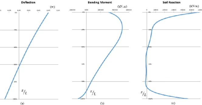
Fig. 5.4 – Curve fitting using Microsoft Excel for the Deflection of the pile (a), Bending Moment (b) and Soil Reaction (c)………51
Fig. 5.5 – Curve fitting using MatLab for the Deflection of the pile (a), Bending Moment (b) and Soil Reaction (c)………...52
Fig. 5.6 – Numerical derivative for the bending moment (b) using the data of the deflection (a)…………53
Fig. 5.7 – Processing of the data exported from PLAXIS 3D………54
Fig. 5.8 – Numerical derivative for the bending moment (b) and soil reaction (c) using the data of the deflection (a)……….55
Fig. 5.9 – Pile represented in SAP2000……….55
Fig. 5.10 – Deflection of the beam……….56
Fig. 5.11– Bending moment along the length of the beam/pile………..56
Fig. 5.12– Different results for bending moment (a) and shear force (b)……….56
Fig. 5.13– p-y curves using the differential equation approach………..57
Fig. 5.14– stress on the soil on the direction parallel to the loading direction………58
Fig. 6.1 – (a) Distribution of front earth pressure and side shear around the pile subjected to lateral load (Zhang et al., 2005); (b) Distribution of stresses around the pile before and after loading (Tuna, 2006)..59
Fig. 6.2 – (a) normal and shear stresses; (b) resulting stresses around the pile………..61
Fig. 6.3 – Interface shear stresses (a), pore pressures (b) and total normal stresses (c)………...61
Fig. 6.4 – Obtained results for xx stresses around the pile using the Interface……….62
Fig. 6.5 – Total stresses in the soil at rest on the xx direction……….63
Fig. 6.6 – Total stresses in the soil with applied displacement on the xx direction………...63
Fig. 6.7 – Effective stresses in the soil with applied displacement on the xx direction……….63
Fig. 6.8 – Pore pressures on the soil with applied displacement………64
Fig. 6.9 – Three- dimensional representation of the stresses on the xx direction at a certain depth…….64
Fig. 6.10 – Upper view of the three- dimensional representation of the stresses on the xx direction at a certain depth……….64
Fig. 6.11 – Two-dimensional development of the horizontal stresses on the xx direction along the model……….65
Fig. 6.12 – Obtained results for xx stresses around the pile using the Soil………...65
Fig. 6.13 – Comparison between the stresses around the pile using the interface and the soil………….66
Fig. 6.14 – Angle used in the empirical curve for the shape of the stresses around the pile………67
Fig. 6.15 – Curve fitting the shape of the stresses around the pile………...…..67
Fig. 6.16 – Curve defining the shape of the stresses around the pile fitting the data from PLAXIS 3D….68 Fig. 6.17 – Typical result for a p-y curve with the different points represented……….68
Fig. 6.18 – p-y curves for different depths……….69
Fig. 6.19 – Fitting of the p-y curve proposed by Matlock for the given data………..70
Fig. 6.20 – Fitting of the p-y curve proposed by Georgiadis for the given data……….71
Fig. 7.1 – API p-y curves for different values of ultimate bearing capacity………74
Fig. 7.2 – Typical evolution of the ultimate bearing capacity of the soil suggested by the API…………75
Fig. 7.3 – Ultimate bearing capacity of the soil over the depth for different values of undrained shear strength using PLAXIS 3D (D=6m)………76
Fig. 7.4 – Comparison between the ultimate bearing capacity of the soil over the depth using the API method and PLAXIS 3D for three different values of constant undrained shear strength over the depth of the soil………77
Fig. 7.5 – Ultimate bearing capacity of the soil over the depth for a variation of the undrained shear strength over the depth of 3 kPa and 4 kPa………...………78
Fig. 7.6 – Ultimate bearing capacity of the soil for different diameters of the pile……….79
Fig. 7.7 – Comparison between the results obtained from PLAXIS 3D and the results of the suggested method of API………80
Fig. 7.8 – Ultimate bearing capacity of the soil for different diameters of the pile for an increase of 3 kPa of undrained shear strength over the depth………..80
Fig. 7.9 – Results obtained from PLAXIS 3D for different diameters with an increase of undrained shear
strength over the depth………81
Fig. 7.10– Results obtained from PLAXIS 3D for different values of Young’s Modulus………..82
Fig. 7.11– Ultimate bearing capacity of the soil over the depth using this new proposed method……….83
Fig. 7.12 – API p-y curves for different values of yc………..84
Fig. 7.13 – Initial stiffness of the p-y curves obtained from PLAXIS 3D for different values of undrained shear strength……….………..85
Fig. 7.14 – Initial stiffness of the p-y curves obtained from PLAXIS 3D for different diameters of the pile………..…86
Fig. 7.15 – Initial stiffness of the p-y curves obtained from PLAXIS 3D for different values of Young’s modulus……….87
Fig. 7.16 – Initial stiffness of the p-y curves normalized by the Young’s modulus………88
Fig. 7.17 – Initial stiffness of the p-y curves normalized by the diameter of the pile……….89
Fig. 7.18 – Initial stiffness of the p-y curves over the depth using this new proposed method………90
Fig. 7.19 – Evolution of the ultimate bearing capacity of the soil over the depth………..91
Fig. 7.20 – p-y curves of the new proposed method……….92
Fig. 7.21 – p-y curves suggested by the API……….92
Fig. 7.22 – Effect of the undrained shear strength of the soil on the p-y curves of the two methods……..93
Fig. 7.23 – Effect of the parameters of deformation of the soil on the p-y curves of the two methods…...93
Fig. 7.24 –p-y curves of the two methods for different diameters………...94
TABLE OF TABLES
Table 3.1 – ε50 and Kpy………...…29
Table 3.2 – Value of Kpy………...34
Table 4.1 – Characteristic stiffness parameters for a Zomergem Clay according to the BSCS………….42
Table 4.2 – Input parameters in PLAXIS 3D for the soil material………42
Table 4.3 – Input parameters in PLAXIS 3D for the plate material……….44
Table 4.4 – Values of Rinter for different types of interactions of soil-structure………..45
SYMBOLS,ACRONYMS AND ABBREVIATIONS
A - Area (m2)
c - Cohesion (kPa) D – Diameter (m)
DNV – Det Norske Veritas E - Elastic Modulus (kPa) E50 – Secant Modulus (kPa)
Eoed -Oedometric Modulus (kPa)
G – Shear modulus (kPa) I- Inertia (m4)
L - Length (m)
k – Subgrade reaction modulus (kN/m2)
ks – Initial stiffness of the p-y curve (kN/m3)
K – Coefficient of subgrade reaction (kN/m3)
K0 - At-rest earth pressure coefficient
M – Bending moment (kN.m) N – Axial force (kN)
P – Soil pressure (kPa) p – Soil reaction (kN/m)
pu – Ultimate bearing capacity (kPa)
Rinter - Reduction of strength at the interface
S – Slope
Su – Undrained shear strength (kPa)
V – Shear force (kN) y – Displacement (y) z - Depth (m)
50 – Strain at one-half of the maximum principal stress difference
- Total stress
- Curvature (m-1)
φ - Friction angle (º) ψ - Dilation angle (º) γ - Unit weight (kN/m3)
γ’ – Submerged unit weight (kN/m3)
1
INTRODUCTION
1.1.FOREWORD
Energy is the main ‘fuel’ for a social and economic development, and technology has become over the last two decades the main driver of this development. The rapid advancement of Information Technology (IT) all over the world has transformed not only the way we think, but also our daily behaviour, and all aspects of human life have been affected by IT and the internet, in particular. Saying this, new ways of producing energy needed to be explored in order for its production could keep up with the development of society and the huge population growth of the last twenty five years (27% between 1993 and 2011).
Energy is the amount of force or power that when applied can move one object from one position to another or Energy defines the capacity of a system to do work and electricity way of energy. Although energy has been known since ancient times, it was never really given a second thought and the first experiments on electricity only appeared 250 years ago (1752) with Benjamin Franklin and his research. The discovery by Faraday of electromagnetic induction occurred almost 80 years later (1831) and it is still somehow used in modern power production – although on much larger scale.
Applications for electricity started to increase since then. It began with the telegraph, light bulb and telephone and continued with radio, television and many other house appliances. This situation led to the searching of new ways of producing energy explaining the increasing use of fuels like coal, gas and oil in power generation. According to the International Energy Agency (2014 Key World Energy Statistics), in 2012 the transports consumed 27.9% and the industry 28.3% of the worlds total produced energy.
The big use of non-renewable energy (energy sources that have a finite quantity and are not able to be replenished) started with the Industrial Revolution. The invention of the internal combustion engine in the 19th century transformed the Western world and led to eventual dependence on fossil fuels. Today,
it is almost impossible to own an item that has been produced without the use of the energy generated by a fossil fuel, nuclear power plants or hydric sources – although nuclear energy is often though as a renewable energy, the uranium deposit on earth is finite and it produces radioactive waste.
Most of non-renewable energy resources have consequences upon the environment. The big emissions of carbon dioxide and other greenhouse gases created what we all know as the increase of the greenhouse effect that is leading to a global warming. The burning of these products also poison waterways and leach harmful toxins into the ground and water.
As these problems began to have a significant impact on the living conditions of our planet, mainly the changes on the weather of the seasons, people and the governments started to take action and try to prevent a catastrophe. The solution is renewable energies.
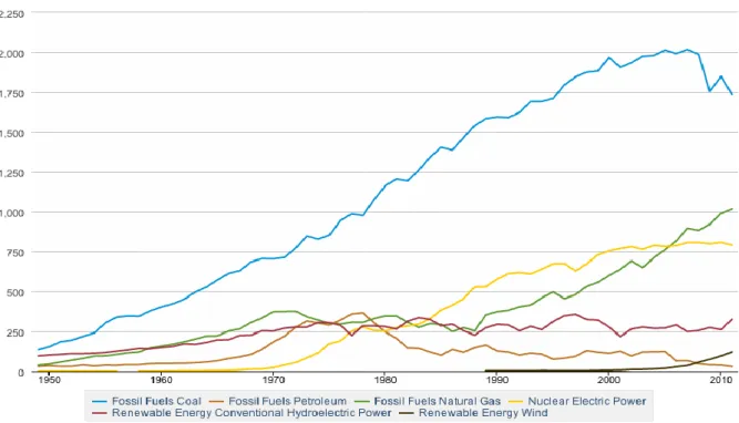
Figure 1.1 shows a comparison between the production of electricity using non-renewable resources and some renewable resources, through the years.
Fig. 1.1 – Comparison between the use of non-renewable and renewable resources to produce electricity, U.S. Energy Information Administration
A renewable energy is defined as an energy that comes from resources which are naturally replenished on a human timescale. Wind is one of these resources, together with sunlight, rain, tides, waves and geothermal heat. It is a source of clean, non-polluting, energy and it is becoming very popular in the last years and lots of investments are being made. The focus of this work is in the wind energy produced offshore. The offshore wind speed average is, more or less, 90% greater than on land.
As the market of offshore wind energy is increasing, many companies seek a more exact and reliable method for the design of the foundations of the wind turbines. When it comes to the lateral-load design, the current methods are based on experiments made on flexible piles while offshore foundations have a more rigid behaviour. This is leading to a lot of investigation by many experts on the field in order to find a more accurate way of describing the lateral load-response behaviour for the soil-pile interaction design. The common way of characterizing this load-response behaviour is through what is usually called as p-y curves.
In the present work, a numerical and theoretical investigation of the soil pile interaction response is made and an analytical solution for the characterization of these p-y curves is suggested as a more accurate method of design for rigid piles that takes into account the diameter of the pile.
1.2.PERSONAL MOTIVATION
Regarding the personal motivation for this work many factors had an important role on it but the one that had the biggest impact was definitely the opportunity of going through such an important stage of my academic career in a recognized and internationalized company like COWI A/S.
The work that will be here presented is the thesis developed as part of the final project of the postgraduate academic master’s degree at the Faculty of Engineering of the University of Porto (FEUP) in the specialization field of Geotechnical Engineering.
An agreement between Prof. Viana da Fonseca, from FEUP, and Ole Hededal, former professor at Danmarks Tekniske Unisersitet – DTU and current Technical Director of the Marine and Foundation Engineering Department of COWI A/S in Lyngby, Denmark, allowed me to move to Denmark and develop my Master’s thesis within an international business environment.
COWI A/S is an engineering, economics and environmental science consulting group with offices all over the world involved in more than 17,000 projects at any given moment anywhere in the planet. It is one of the leading companies when it concerns transportation engineering like tunnels (Abu Hamour surface & groundwater drainage tunnel and the Doha Metro Red Line North Underground, both in Qatar), bridges (Izmit Bay Bridge in Turkey and Puente Nigale in Venezuela) and ports (Al Faw Grand Port in Iraq and Värtahamnen in Sweden) but it also participates in other huge projects (Sonaref Refinery, Angola). When it comes to offshore wind farms COWI also took part of very big projects like the London Array in the UK, the Thornton Bank in Belgium, the Horns Rev in Denmark and the Wikinger in Germany.
The chance of also contributing scientifically with new progresses on the methodology of the design of offshore wind turbine foundations was also a big motivational factor. Working with people who are seen as an international reference on the field of Geotechnical Engineering and contributed for the development and understanding of many unknown soil mechanics and behaviour through published paper on international magazines and conferences was greatly satisfactory.
1.3.OBJECTIVES
The following investigation is focused on a theoretical and numerical investigation of the soil-pile interaction. The purpose is to understand whether the p-y curves used for the design of monopiles foundations should depend on the diameter of these structures or if the current linear relation assumed between the diameter and the resistance of the soil is a correct postulation.
Saying this, the following objectives were established for this work:
Become familiar with geotechnical design approaches for monopile foundation of offshore wind turbines;
Perform literature review of state-of-art on behaviour of monopiles;
Establish a 3D finite element method model (in PLAXIS 3D) of a monopile in uniform soil and simulate its response when loaded;
Use MatLab to process the data obtained from the FEM model and calculate the soil-pile interaction to and applied load or imposed displacement;
Identify the critical parameters based on sensitivity studies;
Propose a new methodology for the characterization of the p-y curves used for the design of monopiles foundations
1.4.STRUCTURE OF THE DOCUMENT
In order to achieve a better organization for the presentation of the previously described objectives, this work was divided into 9 chapters, being this one the first in which a general idea about the thesis scope is given.
The first half of the 2nd Chapter is dedicated to a presentation of the wind energy industry. It is a chapter
explaining how this energy resource was first used, how its technology evolved over the years and its pioneers, its nowadays role on the production of energy to supply the needs of our society and who are the current world leaders on the production of wind energy. A background on how offshore wind farms evolved over the last decades is also presented and, finally, a short introduction on its types of foundations is made.
Second part of Chapter 2 is where a more detailed description of monopiles, one of the types of foundation of offshore wind turbines, is presented. It covers general features like its mechanical characteristics – mostly by comparing rigid piles with flexible piles – but also more detailed aspects like its physical structure and pile testing for lateral loads.
The theoretical background comes in the 3rd Chapter. It starts with an introduction of how the Winkler
method of using springs as a representation of the soil attached to a beam was first used as a method of design for laterally loaded piles and its progress over the years in terms of numerical and analytical solutions. After this, there is an explanation of what p-y curves are followed by a presentation of the suggested methods of characterization of p-y curves developed over the years for cohesive and cohesionless soil.
The 4th Chapter is the description of the 3D FEM model, developed in PLAXIS 3D, that represents a
monopile foundation. This is a very important chapter in a way that every properties of the soil and geometry of the model is presented (and its choice justified) so that, in case of a continuation of the current work by another person, it would be possible to rebuild the models and then intervene on the aspects that wish to be studied (e.g. sensitive studies that were not carried out).
The 5th Chapter is where the forth order differential equation developed by Hetenyi (1947) is explored
as a hypothesis of getting to the subgrade reaction of the soil, p, from the displacement of the pile, y. This equation describes a relationship between the soil reaction and its displacement and it was applied to the results obtain from PLAXIS 3D and complemented with a structural analysis on SAP2000. After labeling the hypothesis explored on the 5th Chapter as unsuitable for the case being here studied,
the 6th Chapter describes how the results obtained from PLAXIS 3D were processed on MatLab and
used to integrate the stresses around the pile in order to find the subgrade reaction of the soil in response to the applied displacement. It is also in this chapter that the resulting p-y curves from the FEM model are presented and the analytical solution for the curve that best fits the obtained outcome is shown. It is also in this chapter that the first comparison between the obtained results and the API method is made. Chapter 7 is dedicated to sensitivity studies on the PLAXIS 3D model and a suggestion for a new method of characterization of the p-y curves. After having defined on the previous chapter that an hyperbola was the type of curve that best fits the results from PLAXIS 3D, some models were run changing some parameters in order to find which ones affect the most the results of the p-y curves. Also, different diameters were tested for the foundations of the monopiles and its effects were explored, which is in fact the main propose of this thesis. Having compared all these sensitivity studies and found consistency of the results, a comparison with the p-y curves from the API is carried out and suggestions to its method are made.
Finally, Chapter 8 summarizes the main conclusions of this thesis and some perspectives of future research are pointed out as important complements for the work that was here developed.
2
WIND ENERGY INDUSTRY
2.1.BACKGROUND AND EVOLUTION
Wind power has been used for human benefits since man started to explore the sea using sailboats. Although sailors didn’t have the physics to help them understanding the mechanics of wind, their empirical achievements were very important for the later development of windmills.
Windmills were the first big progress regarding wind-powered machines and they were used to grind the grains and to pump water. There is few information about this subject from the ancient years so the first known windmills go back to the time of the Persians (500-900 B.C.) and they were used for water pumping. The design was of the vertical axis system – vertical sails attached to a central vertical shaft by horizontal struts (Figure 2.1). These systems were also used in China. They claim that China was the birthplace of windmills and that they were first used more than 2000 years ago but there is no documentation to prove that.
In Europe the first illustrations date back to 1270 A.C. and the design is based in a horizontal axis system with four blades mounted on a central post, much more efficient than the vertical ones. 120 years later the Dutch attached these 'postmills' to a tower (towermill) that used the different floors to different tasks (grinding grain, removing chaff, storing grain, etc). In Greece, in the island of Crete, windmills are still used to pump water for crops and livestock (Figure 2.2).
Fig. 2.1 – Windmills with vertical axis system Fig. 2.2 – Windmills in Crete, Greece
Over the years the windmill sail was improved in many ways and modern designers recognize that after 500 years this process was already completed and all the major features crucial to the performance of modern wind turbine blades were present on these structures. Windmills were very important on the pre-industrial Europe as they were used to several applications like waterwell, irrigation and drainage pumping, grain pumping, saw-milling of timber, and processing of many spices as cocoa, paints and
dyes, and tobacco. During the 19th century, due to the appearance of the steam engines, the use of tower mills declined.
It was only in 1888 that Charles F. Brush first used wind power to produce electrical energy. He incorporated a step-up gearbox in order to turn a direct current generator at its required operational speed but it was still very limited in terms of low-speed and high-solidity rotor for electricity production applications. In 1891, an electrical output wind machine was developed with aerodynamic design principles (resulting in low-solidity rotors) but cheaper and larger fossil-fuel steam plants soon put these machines out of business. In Denmark there were about 2500 windmills by the end of the century and by 1908 there were more than 70 wind-driven electric generators from 5kW to 25kW.
By 1920, the two dominant rotor configurations were labelled as inadequate for generating enough amount of electricity. Yet, small electrical-output wind generators (1 to 3 kilowatts) found a lot of use in the rural areas of the US in some small applications like lighting farms and charge batteries used to power crystal radio sets and later they were extended to refrigerators, freezers, washing machines and power tools. However, due to the increase of the demand of farms for even larger amounts of power and also because the government extended the electrical grid to those areas (because of the New Deal), these systems felt into disuse again. In Australia small hundreds of small wind generators were also produced to provide power at isolated postal service stations and farms.
The world's first megawatt-size wind turbine (1.25MW) was connected to the local electrical distribution system in 1941 (Vermont, USA) and it was only on 1978 that a multi-megawatt wind turbine was created (2MW).
During the Second World War, small wind generators were used to recharge submarine batteries as a fuel-conserving measure. In Europe, after the World War II, the developments on wind energy continue when temporary shortage of fossil fuels led to higher energy costs particularly the post war activity in Denmark and Germany, which was largely important for the future of horizontal axis design of wind turbine.
During the 70s, many people begun to search and rebuilt farm wind generators from the 1930s, as they desired a self-sufficient life-style and solar cells were too expensive for small-scale electrical generation. From 1974 through the mid-1980s the US government worked with industry to advance the technology and enable large commercial wind turbines. Research and developments programs pioneered many of the multi-megawatt turbine technologies in use today. When oil prices declined by a factor of three from 1980 through the early 1990s many turbine manufactures, both large and small, left the business. Energy security, global warming and possible fossil fuel exhaustion led to an expansion of interest in renewable energy at the beginning of the 21st century. Each year more and more investments are made on the wind energy and it is nowadays the fastest developing renewable energy in the world, with the US leading the way. This energy source is considered by many experts as the only renewable energy source which can compete in price with coal and other fossil fuels, and the price of wind power technologies is expected to continue to decline in years to come.
During the year of 2014, 11.791 MW of wind power was installed across the European Union from which 10.308 MW were onshore and 1.483 MW were offshore. The biggest investor country of 2014 was Germany (with more than 5.000 MW), followed by UK (with more than 1.700 MW of which almost 50% were offshore) and then Poland and Sweden both with a little bit more than 1.000 MW.
Overall, during 2014, 26,9 GW of new power generating capacity was installed - 21,3 GW of renewable energy - in EU in which 43,7% were from wind power and 29,7% from Solar Photovoltaic System (8
GW). Since 2000, 412,7 GW of new power capacity has been installed in the EU and of this, 29,4% is from wind power and 56,2% is renewable energy.
Figure 2.3 shows the evolution over the 21th century of the investment of the United States of America on wind energy and Figure 2.4 compares, also in the US, the investment made between the onshore and the offshore wind energy.
Fig. 2.3 – Annual wind power installations in the EU Fig. 2.4 – Annual wind power installations onshore vs offshore
On a global level, 51.477 MW of wind power capacity were installed in 2014. China leads the top 3 with 23.351 MW installed wind power capacity, followed by Germany in second and the USA comes in third place with 4.854 MW. The world total installed wind power capacity is 369,6 GW with China again leading the top 3 with 114,8 GW, followed by the USA with 65,9 GW and then Germany with 39,2 GW.
Denmark, who was once a pioneer in the field of wind energy, is not a world leader anymore. However, its wind turbines delivered in 2014 an equivalent to 39,1% of Danish energy consumption which is a ‘world record’.
In Portugal (Madeira and Azores included), in 2013, the wind power capacity was of 4,731 MW a total share of electricity consumption of 23%, saving nearly 8,182,900 tons of carbon dioxide emissions.
2.2.OFFSHORE WIND ENERGY FARMS
The first wind farm – group of wind turbine at one only location which are interconnected and are used for production of energy – was built in 1980 in New Hampshire. It consisted on 20 wind turbines with a capacity of 30kW each (600kW total) but it is not working anymore. Today, the biggest wind farm in the world is the Gansu Wind Farm in the Gobi desert, China, with a capacity of over 6000 MW of power in 2012 and a goal of 20000 MW by 2020. The largest offshore wind farm in the world is the London Array wind farm in England with a capacity of 630 MW.
In Portugal, the first offshore wind farm near Póvoa de Varzim (the Windfloat farm) is planned to be finished by 2018 and should be able to produce enough energy to provide energy to the whole city of Castelo Branco (40 thousand families).
Wind farms are not an economically viable renewable solution in all parts of the world as they depend a lot on the frequency and speed of the wind. This is the main reason why experts believe that the future of the wind energy lies offshore where winds blow 40 percent more often than on land. Yet, due to extreme weather conditions, offshore wind turbines have much higher construction costs than onshore. Offshore wind farms have significantly smaller negative impact on aesthetics of the landscape compared to wind farms onshore because most offshore wind farms are not visible from shore. When constructing an offshore wind farm it is important to consider whether the nearby ecosystems will be disturbed or not. The interference with shipping lanes or fishing areas must also be taken into account.
Europe has already started huge offshore wind power expansion with the United Kingdom leading the way followed by Germany and Denmark. China is also starting some big investments and the US is seriously considering this clean energy as an option.
Siemens (German multinational conglomerate company and the biggest engineering company in Europe) and Vestas (Danish company and the largest in the world manufacturer, seller, installer and servicer of wind turbines) are the leading turbine suppliers for offshore wind power and DONG Energy (Denmark largest energy company), Vattenfall (a Swedish government’s company) and E.ON (European holding company) are the leading operators.
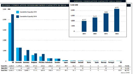
Figure 2.6 shows the biggest producers (countries) of offshore wind energy worldwide and its evolution between the years of 2013 and 2014.
2.3.OFFSHORE WIND TURBINES FOUNDATIONS
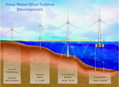
Offshore wind turbines need to be fixed to the seabed with a permanent or semi-permanent support structure. For deep waters a floating structure is used but the most common ones are the fixed foundations used to shallow depths (up to 50 meters). The foundation at the bottom of the turbine transfers loads into the soil so its design is of extreme importance for the good performance of the structure. There are five types of foundations: Jackets; Gravity foundations; Tripods; Tripiles; and Monopiles. Figure 2.7 shows different types of foundations for wind turbines depending on the depth of the water.
Fig. 2.7 – Different types of foundations for offshore wind turbines according to the depth of the water
2.3.1. MONOPILES
Monopiles are large diameter (4 to 6 meters), thick walled, steel tubular structures. They are currently the most common foundation in shallow water (< 30 meter) and will be the scope of this thesis.
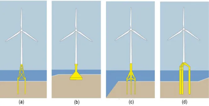
2.3.2. JACKETS
A jacket (Figure 2.8 (a)) is a three or four-legged steel structure with corner piles interconnected with bracing with diameters up to 2 meters to provide the required stiffness. These structures can be used for deep water (100 meters) but, according to the DNV, they should be used between depths of 20 to 50 meters.
2.3.3. GRAVITY FOUNDATIONS
Gravity foundations (Figure 2.8 (b)) are concrete structures that use their weight to resist wind and wave loading. They require a ballast to anchor the foundation and are typically used at sites where installation of piles in the seabed is difficult, such as hard rock or competent soils in shallow depths. Concrete is much cheaper and is more durable in the marine environment than steel so these structures are cost-effective when the environmental loads are low or when additional ballast can be provided at a reasonable cost.
2.3.4. TRIPODS
A tripod (Figure 2.8 (c)) is a relatively lightweight three-legged steel jacket connected to a central pipe foundation that absorbs the wind energy turbine. These structures have good stability and overall stiffness and are suitable for 20 to 80 meters
2.3.5. TRIPILE
The tripile structure (Figure 2.8 (d)) is a three-legged jacked structure in the lower section, connected to a monopile in the upper part of the water column, all made of steel tubes.
Fig. 2.8 – Different types of foundations for offshore wind turbines: jacket (a), gravity base (b), tripod (c) and tripile (d)
2.4.MONOPILES
In up to 30 meters of water with a firm seabed, monopiles are the most commonly form of foundation used nowadays for offshore wind turbines. These giant steel hollow cylindrical tubes range usually from 2,5 to 6 meters in diameter, are 50-60 meters long and weight around 500t (although on deeper sites they can weight more than 800t). It is filled with soil or concrete if a greater resistance is required. Its shape lends itself to simple calculations, straightforward fabrication and tight packing on transport vessels. It is also easier to install at shallow to medium water depths and relatively cheap compared to the other types of foundations.
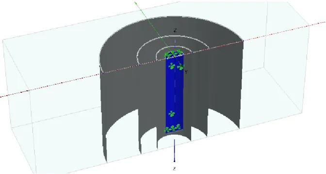
Figure 2.9 (a) shows an installed monopile foundation (dark part under water), with the transition piece already slided in on the top (yellow part), to which the turbine's tower and the rest of the required equipment (access ladders, J-tubes, crane) can be bolted – the description of each of these components will be further given. Figure 2.9 (b) illustrates the transportation of a monopile using trucks and gives an idea of the size of these structures.
Fig. 2.9 – Monopile installed (a) and its transportation (b)
This single pile is driven into the seabed by impact driving (using a hammer blowing system – hydraulic or pneumatic – striking on the protected head of the pile) or by vibratory driving (vibrating pile drivers are fixed at the head of the tube). These equipment operate from a platform that has to be able to keep its correct vertical position. A wind turbine must be designed to resist to its self-weight load – essentially associated to its vertical capacity – and the environmental loads like wind and waves – mostly transversal, therefore conditioning the lateral capacity. The focus of this thesis is directly related to the design of this lateral capacity.
Because of their large diameters, the length/diameter ratio of these monopiles is usually very small. Therefore, these structures tend to behave like short and rigid piles instead of long and flexible ones. There some significant differences of behaviour between these two types of piles: 1) the failure mechanism (Figure 2.10) for the rigid piles is due to the yielding (“fatigue”) of the soil while for the flexible the ultimate load capacity is conditioned by the structural failure of the cross section; 2) while on the toe of the rigid pile there is a “kick” (a small reverse movement), on the flexible pile usually there is no movement on the lower part; 3) the rigid pile has a rotation point, mobilizing active and passive soil pressures over the total length of the pile, whereas the slender pile will deflect around several points (depending mostly on the geomechanical characteristics of the soil layering) leading to soil pressures mostly concentrated in the upper layers, as systematically depicted in Figure 2.11.
The design of rigid piles has been largely discussed over the last years. According to most of the researchers, for the design of flexible piles the best approach is the use of p-y curves. Notwithstanding, for the monopiles of offshore wind turbines – rigid piles systems – although this methodology is not adequate, being less accurate, it has been used frequently with unreliable results. This p-y- method is actually the Winkler model applied on a beam with non-linear springs that represent the soil behaviour for discrete intervals, that is, corresponding to distinct soil layers in depth (which does not mean different types of soils, but different soil behaviour layers, as conditioned by the evolution of the stress state in depth). Finite element method became recently more popular, as it tends to be more representative of the involved factors. Moreover, the codes are becoming more friendly, slowly resolving the trend to use the Winkler method, popular for its simplicity, its ease application and the small required time for the calculation (finite element models are still not very popular for engineering design due to their time-demanding calculations).
2.5.COMPONENTS OF A MONOPILE 2.5.1. TRANSITION PIECE
The transition piece has three different functions: to add a perfect flange on top, to level the transition tower and to provide the whole structure with a boat landing, stairs and a working platform. The process of pile driving (usually hammering) always leads to some tilt of the monopile so the transition piece keeps it perfectly vertical.
It consists of a sleeve, usually with a larger diameter than the monopile (the opposite is possible but impractical for mounting external equipment), placed around it. The overlap length is of 1.5 times the diameter with a gap between the tubes that allows the transition piece to be vertical. The lower and bigger part of it is grouted up to the monopile. This steel cylinder extends between 4 up to 12 meters above sea level.
2.5.2. GROUTED CONNECTION
To fix the transition piece in place, grout (high-strength, fast-curing cement) is injected into the annular gap between the transition piece and the monopile.
The grouted joint (see Figure 2.12) between the transition piece and the monopile must be capable of supporting the weight above it (the transition piece itself, the turbine’s tower and other components) and to resist the compression induced by the bending moments and shear induce by torsion in order for them to be transmitted to the monopile.
The union between the grout and the steel cannot exclusively depend on grout’s adherence to steel. Connectors must be used to assure that the steel and grout work together and they transmit each other the longitudinal shear forces. The quantity and distribution of connectors depend on the resistance capacity of them so a structural analysis must be conducted.
These connectors can be either key connectors or shear connectors, although the first ones lead to stress concentrations around the welded zones and consequently critical areas when considering lifetime estimation of the structure.
2.5.3. EMBEDMENT
The soil in which the monopile is embedded has to be treated as a flexible medium that allows lateral movement and flexure of the pile below seabed. This consideration, which is very realistic, may have big impact on the natural frequency of the structure because its effective fixed level is lower the seabed level.
Monopiles do not need any preparation of the seabed for their installation but are not suited for locations with many boulders in the soil. Still, in the case of encountering a boulder while piling, it is possible to drill it out and blast it with explosives.
The interaction between the pile and the soil is usually modelled using nonlinear lateral springs, known as the p-y curves.
2.5.4. SCOUR
Scour occurs when floodwater passes around an obstruction in the water flow. As the water flows around the object, it must change direction and accelerate. Soil can be loosened and suspended by this process and be carried away.
In the case of monopiles, currents and water motion due to waves will cause significant seabed erosion around it if the seabed is formed of sand or another granular material. This phenomenon would certainly have implications for the stability of the foundations and natural frequency of the support structure. Yet, some projects have been design to accommodate scouring with appropriate allowance in the design for the resulting reductions in the overturning resistance and support structure natural frequency. The occurrence of scour might lead to two problems: damages on the transition piece coating, secondary structures or subsea cables; and the need for occasional replenishment and possible increased environmental impact due to increased volumes of material imported to site.
A design aid for scour whole depth prediction and scour protection design, known as Opti-Pile Design Tool, has been developed and calibrated using model test results and data from existing wind farms. This calculates the size of rock that is stable under maximum current conditions and the required radial extent of the protection.
2.5.5. CORROSION PROTECTION
The approach for corrosion protection is different for the three different zones in which the structure is divided: atmospheric zone, splash zone and submerged zone, which includes the embedded portion. DNV-OS-J101 (design of submarine pipeline systems) requires the steel monopile to be protected by a high quality multi-layered surface coating in the atmospheric zone. In the splash zone, in addition to the surface coating, it requires an extra plate thickness to be provided as a corrosion allowance. Cathodic protection must be provided to the submerged zone together with a 2 mm corrosion allowance in the scour.
2.5.6. CABLE DUCTS
The wind turbine power cables are routed through steel protective tubes known as J tubes, which may be located either inside or outside the transition piece/monopile. The J tubes are so called because they incorporate a 90º bend ate seabed level to enable the cable to exit horizontally.
2.6.MONOPILE DESIGN
The sizing of the monopile is governed by three key factors: resistance to extreme loads, resistance to fatigue loads and tuning of support structure natural frequency to avoid excitation by cyclic loading. Wave and wind fatigue loads depend on the support structure mode shape which in turn depends on the stiffness distribution so the design of monopile against fatigue loads is inevitably an iterative process. It is simpler to develop an initial design based on resistance to extreme wave and wind loads which can then be used to obtain an initial mode shape and set of fatigue loads.
The other key design factor is the restriction on support structure natural frequency and it is often best to take it into account early on in the process of design iteration.
2.7.LATERALLY LOADED PILE TESTING
A horizontal load test on slender piles is carried out to determine the lateral bearing capacity of the soil and the best way to evaluate it is by measuring the bending moment of the pile and then obtain the soil reaction using the second derivative of the bending moment.
For a short and rigid pile the horizontal load test is carried out to determine bearing capacity of the soil, as the failure occurs due to ultimate capacity of the soil. So, if the pile shaft is properly instrumented, it allows the determination of the transfer curves of the side pressure (the so called p-y curves), which best represent the behaviour and failure of the soil.
The most common test procedure is the incremental load test in which the load is applied by steps and in each step the load is kept constant for a certain time, enough to stabilize the associated displacement and measure a reliable value.
The application of the load is made by means of a hydraulic jack and a support to hold the jack horizontally is to be arranged (something heavy enough to stand still). The reaction of the jack is usually provided by another pile or by another set of piles (more commonly two piles connected by a beam). The usual way to measure the displacement along the pile shaft is to install an inclinometer tube along the axis of the pile or to fit strain gauges on various depths of the pile on two opposite peripheral fibres to measure the strains. In both cases the curvature of the pile is obtained, allowing the determination of the bending moments, shear forces and soil pressure by derivation. It is also imperious to measure the absolute value of the displacement of the pile-head, which can be done by topographic means.
The degree of constraint at the pile head must be taken into proper account. During the test, the head of the pile is free to rotate while in real cases the pile cap or a load applied at a higher level (not the ground level) introduces moments at the head.
2.8.FINAL COMMENTS
The relevance of monopiles in nowadays offshore wind structures is, as stated before, very large and it is critical that its design is not oversized as it might lead to extremely high costs. For this reason, many researchers focus on the investigation of the interaction between these pile with large diameters and the surrounding soil in order to better understand this relation and improve its methods of design and achieve better performances.
Big investments are predicted in the industry of offshore wind energy, as this is one of the most clean and cheap renewable energy, so it is essential that this field of engineering is deep explored so that the companies and the governments feel confident to participate in these big projects.
3
THE WINKLER METHOD
AND THE P-Y CURVES
3.1.OVERVIEW
Offshore wind turbines are always subjected to very significant lateral load induced by the waves and by the wind. Therefore, the foundations of these structures are likely to suffer horizontal displacements. A precise prediction of these displacements on these rigid foundations is being investigated by many researchers from all over the world since the second half of the 20th century. For this, two types of
models were developed over the years - discrete models and continuum models – and both have their advantages and disadvantages.
In a discrete model the pile is divided into layers, corresponding to soil layers with prospectively distinct soil-structure interaction response, and in each layer there is a spring (primarily elastic or, more correctly, inelastic) representing the soil interacting with the pile and independent from all the others. This means that the displacement of one point of the pile is not affected by the displacements of the other points. The most famous discrete model is the Winkler model and, nowadays, this methodology has been used by most engineers in design of monopiles foundations, although quite demanding in calculation.
A continuum model takes into account the continuity of the soil so the displacement at any point is influenced by and influences all the other points. The two more common applications of this model is the finite element approach and the elastic continuum approach. Therefore, this type of model is much more realistic, when compared to the Winkler method.
3.2.WINKLER MODEL
Winkler (1867) suggested that the resistance that the ground offers against an external force is proportional to its deflection. He formulated his hypotheses as a beam interacting with a linear elastic support which was later adapted to a pile foundation with a lateral load as these two cases can be perfectly compared (Figure 3.1).
While there are no loads acting on the pile, the surrounding soil remains in at rest stresses state. The idea is that, as the load starts to increase, the structure tends to deviate more and more from its initial position and that introduces additional stresses on the soil. The higher the load, the higher reaction offered by the soil.
This theory was first calibrated for slender (long) piles, although nowadays it has been indiscriminately used for the design of rigid (short) piles with diameters of more than 4 meters, in which their soli-structure interaction differs due to the high rigidity condition.
Fig. 3.1 – a) beam on an elastic support; b) pile foundation with subjected to lateral load
The springs represent the soil, so its deformation and consequently its force should be proportional. This method is also called subgrade reaction method because the constant of the spring can be assumed as the subgrade reaction modulus of the soil [FL-2] (usually denoted by ‘k’). This subgrade reaction
modulus is described as the soil reaction (the force acting in each support point, distanced by one meter), p [FL-1], per unit of displacement, y, (3.1). One other way of representing is by using the coefficient of
subgrade reaction, K [FL-3], which relates the pressure induced by the pile, P[FL-2], with the
displacement (3.2). The diameter of the pile, D, allows an interaction between these two formulations (3.3). The negative sign on the equation indicates that the soil reaction as an opposite direction to the displacement of the pile.
𝑝 = −𝑘. 𝑦 (3.1)
𝑃 = −𝐾. 𝑦 (3.2)
𝑘 = 𝐾. 𝐷 (3.3)
Because of its simplicity the Winkler method does not represent accurately the behaviour of the soil for this kind of problems. The lack of connection and dependency between the springs creates displacement discontinuities between the loaded and the unloaded part of the structure which does not represent the reality (Figure 3.2). This difficulty was later overcome by introducing some interaction between the springs and making the displacements of one spring dependent on the others surrounding it. The problem can be solved analytically or numerically. Yet the analytical solution has much more limitations than the numerical one, although it is easier to apply.
Fig. 3.2 – a) lack of connection between springs; b) interaction between springs – reality
3.2.1. ANALYTICAL SOLUTION
Hetenyi (1946) developed a wave equation (3.4a) – affected by attenuation using the sine and cosine function – that represents the beam-on-foundation concept for the most generic case, which is an infinite beam.
The constants of the equation (C1, C2, C3 and C4) are dependent of the boundary conditions imposed to the problem. Therefore, in order to adapt it to the current problem, it is necessary to consider specific boundary conditions like ‘y=0 for x=∞’ (for this condition C1=C2=0). λ is given by the equation (3.4b) and it is equal to the inverse of the elastic length, Le and k is the subgrade reaction modulus of the soil.
𝑦 = 𝑒𝜆𝑧(𝐶
1cos 𝜆𝑧 + 𝐶2sin 𝜆𝑧) + 𝑒−𝜆𝑧(𝐶3cos 𝜆𝑧 + 𝐶4sin 𝜆𝑧) (3.4a)
𝜆 = √ 𝑘 4𝐸𝐼
4
= 1
𝐿𝑒 (3.4b)
According to Broms (1964), for a pile with a free head, if the length of the pile, L, divided by β (equation (3.5)) is higher than 3.5 the pile is considered long or slender, if it is lower than 2 the pile is short or rigid. 𝛽 = (𝐸𝐼 𝑘) 1 4 ⁄ (3.5)
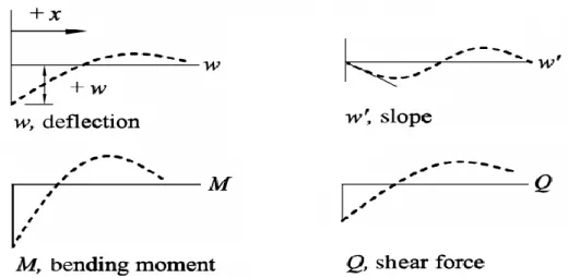
Equation (3.6) is the solution for a semi-infinite beam and Figure 3.3 shows the curves which strictly represent a slender pile. It is possible to obtain the shear force and the bending moment along the beam by triple and double derivation, respectively, of the deflection y (w in the figure). In equation (3.6), P is the applied force, E is the Young’s modulus of the beam and I is the rotational inertia of the beam.
𝑦 = 𝑃
Fig. 3.3 – deflection, slope, bending moment and shear force curves for a semi-infinite beam using equation (3.6)
For slender and long piles, this type of solution is reasonable and very useful, since it gives the exact curves of deflection, bending moment and shear force. For a rigid and short pile this analytical solution is far from being accurate so other options must be found. This method is very limited because it does not allow, for example, the variation of the subgrade reaction modulus with depth, neither the consideration of non-linear behaviour of the soil.
3.2.2. NUMERICAL SOLUTION
The governing equation for the beam-on-foundation Winkler method is a forth order differential equation (3.7) that was developed by Hetenyi (1946). Knowing that the vertical load (N) is very small when compared to its critical buckling load this part of the equation is always despised so it’s possible to get a more simplified equation that is actually used for the calculations. Equation (3.8) is obtained from equation (3.7) and equation (3.1).
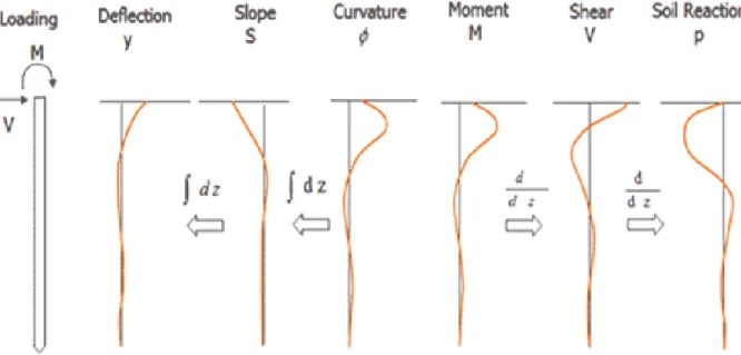
𝐸. 𝐼.𝑑4𝑦 𝑑𝑧4+ 𝑁. 𝑑2𝑦 𝑑𝑧2 = 𝑝(𝑧, 𝑦) (3.7) 𝐸. 𝐼.𝑑4𝑦 𝑑𝑧4+ 𝑘. 𝑦 = 0 (3.8)
By using this forth order differential equation it is possible to obtain significant information about the problem. By solving of this equation, the curve of the soil pressure surrounding the pile can be obtained by integration, being also possible to get the curves of the shear forces, bending moments and the deflection along the pile. The critical design issue for pile foundations is generally the maximum bending moment installed on the pile, rather than its deflection, so this integration is really important. The relation between these curves is explained in Figure 3.4 and the following equations.