Learning the structure of Bayesian networks

(1)

Research Article

Learning the Structure of Bayesian Networks: A Quantitative

Assessment of the Effect of Different Algorithmic Schemes

Stefano Beretta ,

1

Mauro Castelli ,

2

Ivo Gonçalves,

3

Roberto Henriques,

2

and Daniele Ramazzotti

4

1_{DISCo, Universitá degli Studi di Milano-Bicocca, 20126 Milano, Italy}

2_{NOVA Information Management School (NOVA IMS), Universidade Nova de Lisboa, Campus de Campolide,}

1070-312 Lisboa, Portugal

3_{INESC Coimbra, DEEC, University of Coimbra, Coimbra, Portugal} 4_{Department of Pathology, Stanford University, Stanford, California, USA}

Correspondence should be addressed to Daniele Ramazzotti; daniele.ramazzotti@stanford.edu Received 7 June 2018; Revised 1 August 2018; Accepted 7 August 2018; Published 12 September 2018 Academic Editor: Eulalia Martínez

Copyright © 2018 Stefano Beretta et al. This is an open access article distributed under the Creative Commons Attribution License, which permits unrestricted use, distribution, and reproduction in any medium, provided the original work is properly cited. One of the most challenging tasks when adopting Bayesian networks (BNs) is the one of learning their structure from data. This task is complicated by the huge search space of possible solutions and by the fact that the problem is NP-hard. Hence, a full enumeration of all the possible solutions is not always feasible and approximations are often required. However, to the best of our knowledge, a quantitative analysis of the performance and characteristics of the different heuristics to solve this problem has never been done before. For this reason, in this work, we provide a detailed comparison of many different state-of-the-art methods for structural learning on simulated data considering both BNs with discrete and continuous variables and with different rates of noise in the data. In particular, we investigate the performance of different widespread scores and algorithmic approaches proposed for the inference and the statistical pitfalls within them.

1. Introduction

Bayesian networks (BNs) have been applied to several di

ﬀer-entﬁelds, ranging from the water resource management [1]

to the discovery of gene regulatory networks [2, 3]. The task of learning a BN can be divided into two subtasks: (1)

struc-tural learning, i.e., identiﬁcation of the topology of the BN,

and (2) parametric learning, i.e., estimation of the numerical parameters (conditional probabilities) for a given network topology. In particular, the most challenging task of the two is the one of learning the structure of a BN. Diﬀerent methods have been proposed to face this problem, and they

can be classiﬁed into two categories [4–6]: (1) methods based

on detecting conditional independences, also known as constraint-based methods, and (2) score + search methods, also known as score-based approaches. It must be noticed that hybrid methods have also been proposed in [7] but, for

the sake of clarity, here, we limit our discussion to the two mainstream approaches to tackle the task.

As discussed in [8], the input of the former algorithms is a set of conditional independence relations between subsets of variables, which are used to build a BN that represents a large percentage (and, whenever possible, all) of these rela-tions [9]. However, the number of conditional independence tests that such methods should perform is exponential and, thus, approximation techniques are required.

Although constraint-based learning is an interesting approach, as it is close to the semantic of BNs, most of the developed structure learning algorithms fall into the score-based method category, given the possibility of formulating such a task in terms of an optimization problem. As the name implies, these methods have two major components: (1) a scoring metric that measures the quality of every candidate BN with respect to a dataset and (2) a search procedure to Volume 2018, Article ID 1591878, 12 pages

(2)

intelligently move through the space of possible networks, as this space is enormous. More in detail, as shown in [10, 11], searching this space for the optimal structure is an NP-hard problem, even when the maximum number of parents for each node is constrained.

Hence, regardless of the strategy to learn the structure, one wishes to pursue, greedy local search techniques and heuristic search approaches need to be adopted to tackle the problem of inferring the structure of BNs. However, to the best of our knowledge, a quantitative analysis of the per-formance of these diﬀerent techniques has never been done. For this reason, here, we provide a detailed assessment of the performance of diﬀerent state-of-the-art methods for structural learning on simulated data, considering both BNs

with discrete and continuous variables and with diﬀerent

rates of noise in the data. More precisely, we investigate the

characteristics of diﬀerent scores proposed for the inference

and the statistical pitfalls within both the constraint-based and score-based techniques. Furthermore, we study the impact of various heuristic search approaches, namely, hill climbing, tabu search, and genetic algorithms.

We notice that, although we here aim to cover some of the main ideas in the area of structure learning of BNs, sev-eral interesting topics are beyond the scope of this work [12]. In particular, we refer to a more general formulation of the problem [6], and we do not consider, for example, con-texts where it is possible to exploit prior knowledge in order

to make the tasks computationally aﬀordable [13]. At the

same time, in this work, we do not investigate in detail per-formance related to causal interpretations of the BNs [14].

This work extends previous investigation performed in the same area [15, 16] and is structured as follows. In the next two sections, we provide a background on both Bayesian net-works and heuristic search techniques (see Section 2 and Sec-tion 3). In SecSec-tion 4, we describe the results of our study, and in Section 5, we conclude the paper.

2. Bayesian Networks

BNs are graphical models representing the joint distribution over a set of n random variables through a direct acyclic graph (DAG) G = V, E , where the n nodes in V represent the variables, and the arcs E encode any statistical dependence among them. Similarly, the lack of arcs among variables subsumes statistical independence. In this DAG, the set of variables with an arc toward a given node X ∈ V is its set

π X of “parents.” Formally, a Bayesian network [6] is

deﬁned as a pair G, θ over the variable V, with arcs E ⊆ V × V and real-valued parameter θ. When the structure of a BN is known, it is possible to compute the joint distribution of all the variables as the product of the conditional distribu-tions on each variable given its parents.

p X1,… , Xn =

n Xi=1

p Xi∣ π Xi , p Xi∣ π Xi =θXi∣π Xi ,

1

whereθ_X_i_{∣π X}_i is a probability density function.

However, even if we consider the simplest case of binary variables, the number of parameters in each conditional probability table is still exponential in size. For example, in the case of binary variables, the total number of parameters needed to compute the full joint distribution is of size

∑X∈V2π X , where π X is the cardinality of the parent

set of each node. Notice that, if a node does not have parents, the total number of parameters to be computed is 1, which corresponds to its marginal probability.

Moreover, the usage of the symmetrical notion of condi-tional dependence poses further limitations to the task of learning the structure of a BN: two arcs A → B and B → A in a network can in fact equivalently denote dependence between variables A and B; this leads to the fact that two

DAGs having a diﬀerent structure can sometimes model

an identical set of independence and conditional indepen-dence relations (I-equivalence). This yields to the concept of Markov equivalence class as a partially directed acyclic graph where the arcs that can take either orientation are left undirected [6]. In this case, all the structures within

the Markov equivalence class are equivalently “good” in

representing the data, unless a causal interpretation of the BN is given [17].

In the literature, there are two families of methods to learn the structure of a BN from data. The idea behind the ﬁrst group of methods is the one of learning the conditional independence relations of the BN from which, in turn, the network is learned. These methods are often referred to as constraint-based approaches. The second group of methods, the so-called score-based approaches, formulates the task of structure learning as an optimization problem, with scores aimed at maximizing the likelihood of the data given the model. However, both the approaches are known to lead to NP-hard formulations and, because of this, heuristic methods

need to be used to ﬁnd near optimal solutions with high

probability, in a reasonably small number of iterations.

2.1. Constraint-Based Approaches. We now brieﬂy describe

the main idea behind this class of approaches. For a detailed discussion of this topic, we refer to [9, 18].

This class of methods is aimed at building a graph struc-ture to reﬂect the dependence and independence relations in the data that match the empirical distribution. Notwith-standing, the number of conditional independence tests that such algorithms would have to perform among any pair of nodes to test all possible relations is exponential and, because of this, the introduction of some approximations is required. We now provide some details on two constraint-based

algorithms that have been proven to be eﬃcient and of

wide-spread usage: the PC algorithm [9] and the Incremental Asso-ciation Markov Blanket (IAMB) [18].

2.1.1. The PC Algorithm. This algorithm [9] starts with a fully connected graph and, on the basis of pairwise independence tests, it iteratively removes all the extraneous edges. To avoid an exhaustive search of separating sets, the edges are ordered to consider the correct ones early in the search. Once a sepa-rating set is found, the search for that pair ends. The PC algo-rithm orders the separating sets by increasing values of size l,

(3)

starting from 0 (the empty set) until l = n − 2 (where n is the number of variables). The algorithm stops when every vari-able has less than l − 1 neighbors since it can be proven that all valid sets must have already been chosen. During the com-putation, the bigger the value of l is, the larger the number of separating sets must be considered. However, as l gets big, the number of nodes with degree l or higher must have dwindled considerably. Thus, in practice, we only need to consider a small subset of all the possible separating sets.

2.1.2. Incremental Association Markov Blanket Algorithm. Another constraint-based learning algorithm uses the Mar-kov blankets [6] to restrict the subset of variables to test for independence. Thus, when this knowledge is available in advance, we do not need to test a conditioning on all possible

variables. A widely used and eﬃcient algorithm for Markov

blanket discovery is IAMB which, for each variable X, keeps

track of a hypothesis setH X , which is the set of nodes that

may be parents of X. The goal is, for a given H X , to obtain at the end of the algorithm, a Markov blanket of X equals to B X . IAMB consists of a forward and a backward phase. During the forward phase, it adds all the possible variables

into H X that could be in B X , while in the backward

phase, it removes all the false positive variables from the

hypothesis set, leaving the true B X . The forward phase

begins with an emptyH X for each X. Then, iteratively,

variables with a strong association with X (conditioned on

all the variables in H X ) are added to the hypothesis set.

This association can be measured by a variety of nonnegative

functions, such as mutual information. As H X grows

large enough to include B X , the other variables in the

network will have very little association with X, conditioned

onH X . At this point, the forward phase is complete. The

backward phase starts withH X that contains B X and

false positives, which will have small conditional associations, while true positives will associate strongly. Using this test, the backward phase is able to iteratively remove the false positives, until all but the true negatives are eliminated. 2.2. Score-Based Approaches. These approaches is aimed at

maximizing the likelihood L of a set of observed data D,

which can be computed as the product of the probability of each observation. Since we want to infer a model G that best explains the observed data, we deﬁne the likelihood of observing the data given a speciﬁc model G as

LL G ; D =

d∈D

P d ∣ G ₂

Practically, however, for any arbitrary set of data, the most likely graph is always the fully connected one, since adding an edge can only increase the likelihood of the data, i.e., this approach overﬁts the data. To overcome this limita-tion, the likelihood score is almost always combined with a regularization term that penalizes the complexity of the model in favor of sparser solutions [6].

As already mentioned, such an optimization problem leads to intractability, due to the enormous search space of the valid solutions. Because of this, the optimization task is

often solved with heuristic techniques. Before moving on to describe the main heuristic methods employed to face such complexity (see Section 3), we now give a short description of a particularly relevant and known score, called Bayesian Information Criterion (BIC) [19], as an example of scoring function adopted by several the score-based methods. 2.2.1. The Bayesian Information Criterion. BIC uses a score that consists of a log-likelihood term and a regularization term that depend on a model G and data D:

BIC G ; D =LL G ; D − log m

2 dim G , 3

where D denotes the data, m denotes the number of samples, and dim G denotes the number of parameters in the model. We recall that in this formulation, the BIC score should be maximized. Since, in general, dim · depends on the number of parents of each node, it is a good metric for model plexity. Moreover, each edge added to G increases the com-plexity of the model. Thus, the regularization term based on dim · favors graphs with fewer edges and, more speciﬁcally, fewer parents for each node. The term log m/2 essentially weighs the regularization term. The eﬀect is that the higher

the weight, the more sparsity will be favored over

“explain-ing” the data through maximum likelihood.

Notice that the likelihood is implicitly weighted by the number of data points since each point contributes to the score. As the sample size increases, both the weight of

the regularization term and the “weight” of the likelihood

increase. However, the weight of the likelihood increases fas-ter than that of the regularization fas-term. This means that, with more data, the likelihood will contribute more to the score, and we may trust our observations more and have less need for regularization. Statistically speaking, BIC is a consistent score [6]. Consequently, G contains the same independence relations as those implied by the true structure.

3. Heuristic Search Techniques

We now describe some of the main state-of-the-art search strategies that we took into account in this work. In particu-lar, as stated in Section 1, we considered the following search methods: hill climbing, tabu search, and genetic algorithms. 3.1. Hill Climbing. Hill climbing (HC) is one of the simplest iterative techniques that have been proposed for solving opti-mization problems. While HC consists of a simple and intu-itive sequence of steps, it is a good search scheme to be used as a baseline for comparing the performance of more advanced optimization techniques.

Hill climbing shares with other techniques (like simu-lated annealing [20] and tabu search [21]) the concept of neighborhood. Search methods based on this latter concept are iterative procedures in which a neighborhood N i is

deﬁned for each feasible solution i, and the next solution

j is searched among the solutions in N i . Hence, the

neigh-borhood is a function N S → 2S that assigns to each

(4)

The sequence of steps of the hill climbing algorithm, for a maximization problem w.r.t. a given objective function f , are the following:

(1) Choose an initial solution i in S

(2) Find the best solution j in N i (i.e., the solution j such that f j ≥ f k for every k in N i )

(3) If f j < f i , then stop; else, set i = j and go to step 2 As it is clear from the aforementioned algorithm, hill climbing returns a solution that is a local maximum for the problem at hand. This local maximum does not gener-ally correspond to the global minimum for the problem under exam, that is, hill climbing does not guarantee to return the best possible solution for a given problem. To counteract this limitation, more advanced neighborhood

search methods have been deﬁned. One of these methods

is tabu search, an optimization technique that uses the

con-cept of“memory.”

3.2. Tabu Search. Tabu search (TS) is a metaheuristic that guides a local heuristic search procedure to explore the solu-tion space beyond local optimality. One of the main compo-nents of this method is the use of an adaptive memory, which

creates a moreﬂexible search behavior. Memory-based

strat-egies are therefore the main feature of TS approaches,

founded on a quest for “integrating principles,” by which

alternative forms of memory are appropriately combined with eﬀective strategies for exploiting them.

Tabus are one of the distinctive elements of TS when compared to hill climbing or other local search methods. The main idea in considering tabus is to prevent cycling when moving away from local optima through nonimprov-ing moves. When this situation occurs, somethnonimprov-ing needs to be done to prevent the search from tracing back its steps to where it came from. This is achieved by declaring tabu

(disallowing) moves that reverse the eﬀect of recent moves.

For instance, let us consider a problem where solutions are binary strings of a prefixed length, and the neighborhood of a solution i consists of the solutions that can be obtained from i by flipping only one of its bits. In this scenario, if a solution j has been obtained from a solution i by changing one bit b, it is possible to declare a tabu to avoid to flip back the same bit b of j for a certain number of iterations (this number is called the tabu tenure of the move). Tabus are also useful to help in moving the search away from previously vis-ited portions of the search space and, thus, perform more extensive exploration.

As reported in [22], tabus are stored in a short-term memory of the search (the tabu list) and usually, only a ﬁxed limited quantity of information is recorded. It is pos-sible to store complete solutions, but this has a negative impact on the computational time required to check whether a move is a tabu or not and, moreover, it requires a vast amount of space. The second option (which is the one commonly used) involves recording the last few transfor-mations performed to obtain the current solution and prohi-biting reverse transformations.

While tabus represent the main distinguished feature of TS, this feature can introduce other issues in the search pro-cess. In particular, the use of tabus can prohibit attractive moves, or it may lead to an overall stagnation of the search process, with a lot of moves that are not allowed. Hence, sev-eral methods for revoking a tabu have been deﬁned [23], and they are commonly known as aspiration criteria. The sim-plest and most commonly used aspiration criterion consists of allowing a move (even if it is tabu) if it results in a solution with an objective value better than that of the current best-known solution (since the new solution has obviously not been previously visited).

The basic TS algorithm, considering the maximization of the objective function f , works as follows:

(1) Randomly select an initial solution i in the search

space S, and set i∗= i and k = 0, where i∗ is the best

solution so far, and k the iteration counter

(2) Set k = k + 1 and generate the subset V of the admis-sible neighborhood solutions of i (i.e., nontabu or allowed by aspiration)

(3) Choose the best j in V and set i = j

(4) If f i > f i∗ , then set i∗= i

(5) Update the tabu and the aspiration conditions (6) If a stopping condition is met, then stop; else, go to

step 2.

The most commonly adopted conditions to end the algo-rithm are when the number of iterations (K) is larger than a maximum number of allowed iterations or if no changes to the best solution have been performed in the last N iterations (as it is in our tests).

Speciﬁcally, in our experiments, we modeled for both HC and TS the possible valid solutions in the search space as a binary adjacency matrix describing acyclic directed graphs. The starting point of the search is the empty graph (i.e., with-out any edge), and the search is stopped when the current best solution cannot be improved with any move in its neighborhood.

The algorithms then consider a set of possible solutions (i.e., all the directed acyclic graphs) and navigate among them by means of 2 moves: insertion of a new edge or removal of an edge currently in the structure. We also recall that in the literature, many alternatives are proposed to nav-igate the search space when learning the structure of Bayesian network (see [24, 25]). But, for the purpose of this work, we preferred to stick with the classical (and simpler) ones. 3.3. Genetic Algorithms. Genetic algorithms (GAs) [26] are a class of computational models that mimic the process of nat-ural evolution. GAs are often viewed as function optimizers although the range of problems to which GAs have been applied is quite broad. Their peculiarity is that potential

solu-tions that undergo evolution are represented asﬁxed length

strings of characters or numbers. Generation by generation, GAs stochastically transform sets (also called populations)

(5)

of candidate solutions into new, hopefully improved,

popu-lations of solutions, with the goal of ﬁnding one solution

that suitably solves the problem at hand. The quality of each

candidate solution is expressed by using a user-deﬁned

objective function calledﬁtness. The search process of GAs

is shown in Figure 1.

To transform a population of candidate solutions into a new one, GAs make use of particular operators that transform the candidate solutions, called genetic opera-tors: crossover and mutation. Crossover is traditionally used to combine the genetic material of two candidate solutions (parents) by swapping a part of one individual (substring) with a part of the other. On the other hand, mutations introduce random changes in the strings repre-senting candidate solutions. In order to be able to use GAs to solve a given optimization problem, candidate solu-tions must be encoded into strings and, often, also the genetic operators (crossover and mutation) must be specialized for the considered context.

GAs have been widely used to learn the BN structure con-sidering the search space of the DAGs. In the large majority of the works [27–32], the GA encodes the connectivity matrix of the BN structure in its individuals. This is the same approach used in our study. Our GA follows the common structure:

(1) Generate the initial population

(2) Repeat the following operations until the total num-ber of generations is reached:

(a) Select a population of parents by repeatedly applying the parent selection method

(b) Create a population of oﬀspring by applying the

crossover operator to each set of parents (c) For each oﬀspring, apply one of the mutation

operators with a given mutation probability (d) Select the new population by applying the

survi-vor selection method

(3) Return the best performing individual

Unless stated otherwise, the following description is valid for both GA variants (discrete and continuous). The initiali-zation method and the variation operators used in our GA ensure that every individual is valid, i.e., each individual is guaranteed to be an acyclic graph. The initialization method creates individuals with exactly N/2 connections between variables, where N is the total number of variables. A con-nection is only added if the graph remains acyclic. The nodes being connected are selected with uniform probabil-ity from the set of variables. In the continuous variant, since the input data is normalized, the value associated with each connection is randomly generated between 0.0 and 1.0, with uniform probability. The crossover operates over two par-ents and returns one oﬀspring. The oﬀspring is initially a

copy of the ﬁrst parent. Afterward, a node with at least

one connection is selected from the second parent and all the valid connections starting from this node are added to

the oﬀspring.

Three mutation operators are considered in our GA implementation: add connection mutation, remove

con-nection mutation, and perturbation mutation. The ﬁrst

two are applied in both GA variants, while the perturba-tion mutaperturba-tion is only applied in the continuous variant. The oﬀspring resulting from the add connection mutation operator diﬀers from the parent in having an additional connection. The newly connected nodes are selected with uniform probability. In the continuous variant, the value associated with the new connection is randomly generated between 0.0 and 1.0 with uniform probability. Similarly,

the oﬀspring resulting from the remove connection

muta-tion operator diﬀers from the parent in having one less

connection. The nodes to be disconnected are selected with uniform probability. The perturbation mutation oper-ator applies Gaussian perturbations to the values associ-ated with at most N/2 connections. The total number of perturbations may be less than N/2 if the individual being mutated has less than N/2 connections. Each value is per-turbed following a Gaussian distribution having mean 0.0

Calculate ﬁtness of individuals Apply genetic operators to create new individuals Randomly create initial population Select individuals based on ﬁtness Maximum number of generations reached? Return best solution Yes No

(6)

and standard deviation 1.0. Any resulting value below 0.0 or above 1.0 is bounded to 0.0 or 1.0, respectively. Regard-less of the GA variant, mutation is applied with a proba-bility of 0.25. When a mutation is being applied, the

speciﬁc mutation operator is selected with uniform

proba-bility from the available options (two in the discrete vari-ant and three in the continuous varivari-ant). The mutation operator of the GA works by applying the perturbation to the existing values associated to each edge of the solu-tions. Since such modiﬁcation to the value should not be highly disruptive, a common choice is to employ a Gauss-ian probability distribution having mean 0 and standard deviation 1.

In terms of parameters, a population of size 100 is used, with the evolutionary process being able to perform 100 generations. Parents are selected by applying a tour-nament of size 3. The survivor selection is elitist in the sense that it ensures that the best individual survives to the next generation.

4. Results and Discussion

We made use of a large set of simulations on randomly generated datasets with the aim of assessing the charac-teristics of the state-of-the-art techniques for structure learning of BNs.

We generated data for both the case of discrete (2 values, i.e., 0 or 1) and continuous (we used 4 levels, i.e., 1, 2, 3, and 4) random variables. Notice that, for computational reasons, we discretized our continuous variables using only 4 catego-ries. For each of them, we randomly generated both the struc-ture (i.e., 100 weakly connected DAGs having 10 and 15 nodes) and the related parameters (we generated random values in (0, 1) for each entry of the conditional probability tables attached to the network structure) to build the simu-lated BNs. We also considered 3 levels of density of the net-works, namely, 0.4, 0.6, and 0.8, of the complete graph. For each of these scenarios, we randomly sampled from the BNs’ several datasets of diﬀerent size, based on the number of nodes. Speciﬁcally, for networks of 10 variables, we gener-ated datasets of 10, 50, 100, and 500 samples, while for 15 variables, we considered datasets of 15, 75, 150, and 750 sam-ples. Furthermore, we also considered additional noise in the samples as a set of random entries (both false positives and false negatives) in the dataset. We recall that, based on sam-ple size, the probability distribution encoded in the generated

datasets may be diﬀerent from the one subsumed by the

related BN. However, here, we also consider additional noise (besides the one due to sample size) due, for example, to errors in the observations. We call noise-free, the datasets in which such an additional noise is not applied. To this extent, we considered noise-free dataset (noise rate equals 0%) and dataset with an error rate of 10% and 20%. In total, this led us to a total number of 14400 random datasets.

For all of them, we considered both the constraint-based and the score-based approaches to structural learning. From the former category of methods, we considered the PC algo-rithm [9] and the IAMB [18]. We recall that these methods return a partially directed graph, leaving undirected the arcs

that are not unequivocally directable. In order to have a fair comparison with the score-based method which returns DAGs, we randomly resolved the ambiguities, by generating random solutions (i.e., DAGs) consistent with the statistical constraints by PC and IAMB (that is, we select a random direction for the undirected arcs).

Moreover, among the score-based approaches, we con-sider 3 maximum likelihood scores, namely, log-likelihood [6], BIC [19], and AIC [33] (for continuous variables we used the corresponding Gaussian likelihood scores). For all of them, we repeated the inference on each conﬁguration by using HC, TS, and GA as search strategies.

This led us to 11 diﬀerent methods to be compared, for a total of 158400 independent experiments. To evaluate the obtained results, we considered both false positives (FP) (i.e., arcs that are not in the generative BN but that are inferred by the algorithm) and false negatives (FN) (i.e., arcs that are in the generative BN but that are not inferred by the algorithm). Also, with TP (true positives) being the arcs in the generative model and TN (true negatives) the arcs that are not in the generative model, for all the experiments, we considered the following metrics:

Precision = TP TP + FP, Recall = TP TP + FN, Specif icity = TN TN + FP, Accuracy = TP + TN TP + FP + TN + Fn 4

4.1. Results of the Simulations. In this section, we com-ment on the results of our simulations. As anticipated,

we computed precision, recall (sensitivity), and speciﬁcity,

as well as accuracy and Hamming distance, to assess the performance and the underfit/overfit trade-off of the differ-ent approaches. Overall, from the obtained results, it is straightforward to notice that methods including more edges in the inferred networks are also more subject to errors in terms of accuracy, which may also resemble a bias of this metric that tends to penalize solutions with false positive edges rather than false negatives. On the other hand, since a typical goal of the problems involving the

inference of BNs is the identiﬁcation of novel relations (that

is, proposing novel edges in the network), underﬁtting

approaches could be more eﬀective in terms of accuracy,

but less useful in practice.

With a more careful look, theﬁrst evidence we obtained

from the simulations is that the two parameters with the highest impact on the inferred networks are the density and the number of nodes (i.e., network size). For this reason, we ﬁrst focused our attention on these two parameters, and we analyzed how the diﬀerent tested combinations of methods and scores behave.

As shown in Figure 2, all the approaches seem to perform better when dealing with low-density networks, in fact, for almost all the methods, the accuracy is higher for density

(7)

equal to 0.4, while it is lower for density equal to 0.8. Since each edge of the network is a parameter that has to be “learned,” it is reasonable to think that the more edges are present in the BN, the harder becomes the problem to be solved when learning it. Moreover, we can also observe that the results in terms of accuracy obtained for BN of discrete variables are slightly better than those achieved on the con-tinuous ones. To this extent, the only outlier is the loglik score combined with hill climbing and with tabu search on datasets with continuous variables, for which the trend is the opposite, w.r.t. that of all the other approaches. In fact, in both these cases, the accuracy is higher on high-density

datasets, and this is likely due to a very high overﬁt of the

approach. It is interesting to notice that genetic algorithms (combined with the loglik score) is less aﬀected by this prob-lem, and this trend will also be shown in the next analyses.

In addition to the accuracy, we also computed the Ham-ming distance between the reconstructed solutions and the BNs used to generate the data, in order to quantify the errors of the inference process. This analysis showed that, besides the network density, also the number of nodes (parameters

to be learned) inﬂuences the results, as reported in Figure 3.

It is interesting to observe that, in the adopted experimental setup, we set the number of samples to be proportional to the number of nodes of the network, that is, for 10 nodes; in the same conﬁgurations, we have a lower number of sam-ples, compared to the ones for 15 nodes. From a statistical point of view alone, we would expect the problem to be easier when having more samples to build the BN, since this would lead to more statistical power and, intuitively, should com-pensate for the fact that with 15 nodes, we have more param-eters to learn than the ones for the case of 10 nodes. While this may be the case (in fact, we have similar accuracy for both 10 and 15 nodes), we also observe a constantly higher

Hamming distance with more nodes. In fact, when dealing with more variables, we observed a shift in the performance, that is, even when the density is low, we observe more errors manifesting with higher values in terms of Ham-ming distance. This is due to the fact that, when increasing the number of variables, we also increase the complexity of the solutions.

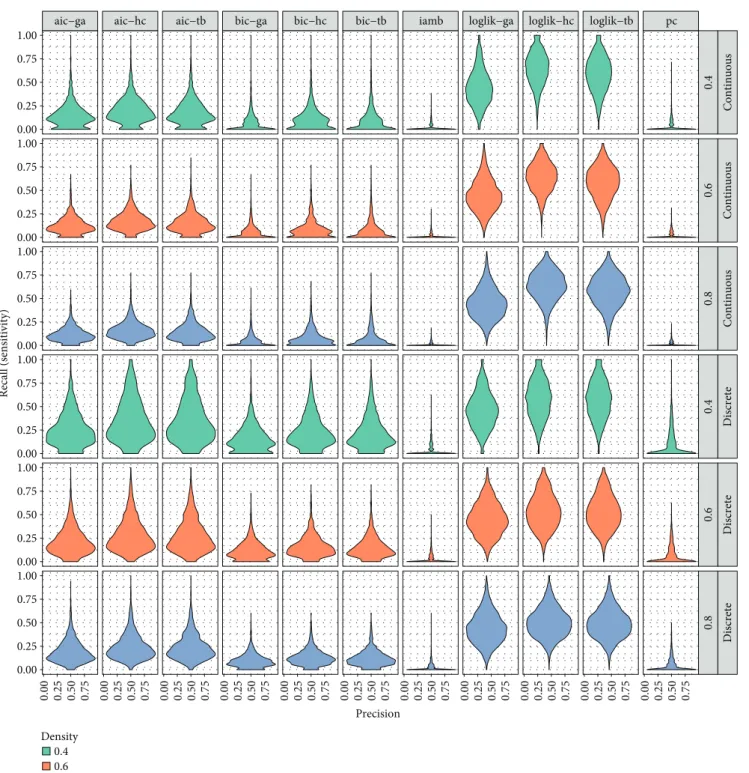
A further analysis we performed was devoted to assessing the impact of both overﬁt and underﬁt. As it is possible to observe from the plots in Figures 4 and 5, we obtain two opposite behaviors, namely, the combinations of scores and

search strategies show evident diﬀerent trends in terms of

sensitivity (recall), speciﬁcity, and precision. In detail, iamb

and pc tend to underﬁt, since they both produce networks

with consistently low density. While they achieve similar (high) results in terms of accuracy (see Figure 2), their trend toward underfit does not make them suited for the identifica-tion of novel edges, rather being more indicated for descrip-tive purposes. On the other hand, the loglik score, (mostly) independently from the adopted search technique, consis-tently overfits. Both these behaviors can be observed in the violin plots of Figures 4 and 5: for each density, we can observe that iamb/pc results have very low recall values, while the distribution of the results of the loglik score is centered on higher values.

The other two scores, i.e., AIC and BIC, present a better

trade-off between overfit and underfit, with BIC being less

affected by the overfit, while AIC reconstructing slightly denser networks. Once again, this trade-off between the two regularizators is well known in the literature and points to AIC being more suited for predictions while BIC for descriptive purposes.

Another relevant result of our analysis is the characteri-zation of the performance of genetic algorithms in terms of

0.25 0.50 0.75 1.00 0.25 0.50 0.75 1.00 Accuracy

aic−ga aic−hc aic−tb bic−ga bic−hc bic−tb iamb loglik−ga loglik−hc loglik−tb pc

Continuous Discrete Density 0.4 0.6 0.8

Figure 2: Boxplots showing the accuracy of the results obtained by the 11 tests approaches on the discrete and continuous datasets. In the ﬁgure, conditional boxplot in each subpanel reports results for structure of density 0.4, 0.6, and 0.8 from left to right.

(8)

sensitivity (recall). Speciﬁcally, it must be noticed that for all the three regularizators, genetic algorithms achieve similar results of both precision and speciﬁcity if compared with both hill climbing and tabu search, but in terms of sensitivity

(recall), it presents reduced overﬁt. In fact, as it is possible

to observe in the plots of Figures 4 and 5 for each score (i.e., loglik, AIC, and BIC), the sensitivity results of genetic algorithms are lower than those of both hill climbing and

tabu search, highlighting the reduced impact of overﬁt.

In summary, we can draw the following conclusions. (i) Dense networks are harder to learn (see Figure 2) (ii) The number of nodes aﬀects the complexity of the

solutions, leading to higher Hamming distance (number of errors) even if with similar accuracy (see Figures 2 and 3)

(iii) Networks with continuous variables are harder to learn compared to the binary ones (see Figure 2)

(iv) iamb and pc algorithms tend to underﬁt, while loglik overﬁts (see Figures 4 and 5)

(v) Genetic algorithms tend to reduce underﬁt (see Figures 4 and 5)

We conclude the section by providing p values by Mann– Whitney U test [34] in support of such claims in Table 1. The claim for greater and less values, i.e., accuracy, is performed with the one-tail test alternatives.

The tests are performed on all the conﬁgurations of our simulations.

5. Conclusions

Bayesian networks are a widespread technique to model dependencies among random variables. A challenging prob-lem when dealing with BNs is the one of learning their struc-tures, i.e., the statistical dependencies in the data, which may sometime pose a serious limit to the reliability of the results.

10 Continuous 15 Continuous 10 Discrete 15 Discrete 0 ₂₅ ₅₀ ₇₅ 0 ₂₅ ₅₀ ₇₅ 0 ₂₅ ₅₀ ₇₅ 0 ₂₅ ₅₀ ₇₅ 0 ₂₅ ₅₀ ₇₅ 0 ₂₅ ₅₀ ₇₅ 0 ₂₅ ₅₀ ₇₅ 0 ₂₅ ₅₀ ₇₅ 0 ₂₅ ₅₀ ₇₅ 0 ₂₅ ₅₀ ₇₅ 0 ₂₅ ₅₀ ₇₅ 0 100 200 300 0 100 200 300 0 100 200 300 0 100 200 300 Hamming distance Count Density 0.4 0.6 0.8

Figure 3: Bar plots showing the Hamming distances of the solutions obtained by the 11 tested approaches, grouped by type of dataset (discrete and continuous) and number of nodes of the network (10 and 15), while colors represent densities (0.4, 0.6, and 0.8).

(9)

Despite their extensive use in a vast set ofﬁelds, to the best of our knowledge, a quantitative assessment of the per-formance of diﬀerent state-of-the-art methods to learn the structure of BNs has never been performed. In this work,

we aim to go in the direction ofﬁlling this gap and we

pre-sented a study of diﬀerent state-of-the-art approaches for

structural learning of Bayesian networks on simulated data, considering both discrete and continuous variables.

To this extent, we investigated the characteristics of 3 dif-ferent likelihood scores, combined with 3 commonly used search strategy schemes (namely, genetic algorithms, hill climbing, and tabu search), as well as 2 constraint-based tech-niques for the BN inference (i.e., iamb and pc algorithms).

Our analysis identiﬁed the factors having the highest

impact on the performance, that is, density, number of vari-ables, and variable type (discrete vs continuous). In fact, as

0.4 Continuous 0.6 Continuous 0.8 Continuous 0.4 Discrete 0.6 Discrete 0.8 Discrete 0.00 0.25 0.50 0.75 0.00 0.25 0.50 0.75 0.00 0.25 0.50 0.75 0.00 0.25 0.50 0.75 0.00 0.25 0.50 0.75 0.00 0.25 0.50 0.75 0.00 0.25 0.50 0.75 0.00 0.25 0.50 0.75 0.00 0.25 0.50 0.75 0.00 0.25 0.50 0.75 0.00 0.25 0.50 0.75 0.00 0.25 0.50 0.75 1.00 0.00 0.25 0.50 0.75 1.00 0.00 0.25 0.50 0.75 1.00 0.00 0.25 0.50 0.75 1.00 0.00 0.25 0.50 0.75 1.00 0.00 0.25 0.50 0.75 1.00 Precision Recall (sensitivity) Density 0.4 0.6 0.8

Figure 4: Violin plots showing precision and recall of the solutions obtained by the 11 tested approaches, grouped by the type of dataset (discrete and continuous) and density values (0.4, 0.6, and 0.8).

(10)

shown here, these settings affect the number of parameters to be learned, hence complicating the optimization task. Fur-thermore, we also discussed the overfit/underfit trade-off of

the diﬀerent tested techniques with the constraint-based

approaches showing trends toward underﬁtting and the

loglik score showing high overﬁt. Interestingly, in all the

con-ﬁgurations, genetic algorithms showed evidence of reducing

the overﬁt, leading to denser structures.

Overall, we place our work as a starting eﬀort to better characterize the task of learning the structure of Bayesian networks from data, which may lead in the future to a more eﬀective application of this approach. In particular, we focused on the more general task of learning the structure of a BN [6], and we did not dwell on several interesting

domain-speciﬁc topics, which we leave for future

investiga-tions [12–14].

Density 0.4 0.6 0.8

0.4 Continuous 0.6 Continuous 0.8 Continuous 0.4 Discrete 0.6 Discrete 0.8 Discrete 0.00 0.25 0.50 0.75 1.00 0.00 0.25 0.50 0.75 1.00 0.00 0.25 0.50 0.75 1.00 0.00 0.25 0.50 0.75 1.00 0.00 0.25 0.50 0.75 1.00 0.00 0.25 0.50 0.75 1.00 0.00 0.25 0.50 0.75 1.00 0.00 0.25 0.50 0.75 1.00 0.00 0.25 0.50 0.75 1.00 0.00 0.25 0.50 0.75 1.00 0.00 0.25 0.50 0.75 1.00 0.00 0.25 0.50 0.75 1.00 0.00 0.25 0.50 0.75 1.00 0.00 0.25 0.50 0.75 1.00 0.00 0.25 0.50 0.75 1.00 0.00 0.25 0.50 0.75 1.00 0.00 0.25 0.50 0.75 1.00 Speciﬁcity Sensitivity (recall)

Figure 5: Violin plots showing speciﬁcity and sensitivity of the solutions obtained by the 11 tested approaches, grouped by the type of dataset (discrete and continuous) and density values (0.4, 0.6, and 0.8).

(11)

Data Availability

The datasets used to support theﬁndings of this study are

available from the corresponding author upon request.

Conflicts of Interest

The authors declare that they have no conﬂicts of interest.

Acknowledgments

This work was also ﬁnanced through the Regional

Opera-tional Programme CENTRO2020 within the scope of the project CENTRO-01-0145-FEDER-000006.

References

[1] S.-S. Leu and Q.-N. Bui, “Leak prediction model for water distribution networks created using a Bayesian network learning approach,” Water Resources Management, vol. 30, no. 8, pp. 2719–2733, 2016.

[2] F. Dondelinger, S. Lèbre, and D. Husmeier, “Non-homoge-neous dynamic Bayesian networks with Bayesian regulariza-tion for inferring gene regulatory networks with gradually time-varying structure,” Machine Learning, vol. 90, no. 2, pp. 191–230, 2013.

[3] W. Young, A. E. Raftery, and K. Yeung, “Fast Bayesian inference for gene regulatory networks using ScanBMA,” BMC Systems Biology, vol. 8, no. 1, p. 47, 2014.

[4] W. Buntine,“A guide to the literature on learning probabilistic networks from data,” IEEE Transactions on Knowledge and Data Engineering, vol. 8, no. 2, pp. 195–210, 1996.

[5] R. Daly, Q. Shen, and S. Aitken,“Learning Bayesian networks: approaches and issues,” The Knowledge Engineering Review, vol. 26, no. 02, pp. 99–157, 2011.

[6] D. Koller and N. Friedman, Probabilistic Graphical Models: Principles and Techniques, MIT Press, 2009.

[7] G. A. P. Saptawati and B. Sitohang, “Hybrid algorithm for learning structure of Bayesian network from incomplete data-bases,” in IEEE International Symposium on Communications and Information Technology, 2005. ISCIT 2005, pp. 741–744, Beijing, China, 2005, IEEE.

[8] P. Larrañaga, H. Karshenas, C. Bielza, and R. Santana, “A review on evolutionary algorithms in Bayesian network learn-ing and inference tasks,” Information Sciences, vol. 233, pp. 109–125, 2013.

[9] P. Spirtes, C. N. Glymour, and R. Scheines, Causation, Predic-tion, and Search, MIT press, 2000.

[10] D. M. Chickering,“Learning Bayesian networks is NP-com-plete,” in Learning from Data, pp. 121–130, Springer, 1996. [11] D. M. Chickering, D. Heckerman, and C. Meek,“Large-sample

learning of Bayesian networks is NP-hard,” Journal of Machine Learning Research, vol. 5, pp. 1287–1330, 2004.

[12] M. Drton and M. H. Maathuis,“Structure learning in graphical modeling,” Annual Review of Statistics and Its Application, vol. 4, no. 1, pp. 365–393, 2017.

[13] F. M. Stefanini,“Chain graph models to elicit the structure of a Bayesian network,” The Scientiﬁc World Journal, vol. 2014, Article ID 749150, 12 pages, 2014.

[14] C. Heinze-Deml, M. H. Maathuis, and N. Meinshausen, “Causal structure learning,” Annual Review of Statistics and Its Application, vol. 5, no. 1, pp. 371–391, 2018.

[15] S. Beretta, M. Castelli, I. Gonçalves, I. Merelli, and D. Ramazzotti, “Combining Bayesian approaches and evolu-tionary techniques for the inference of breast cancer networks,” in Proceedings of the 8th International Joint Conference on Com-putational Intelligence, pp. 217–224, Porto, Portugal, 2016. [16] S. Beretta, M. Castelli, and R. Dondi,“Parameterized

tractabil-ity of the maximum-duo preservation string mapping prob-lem,” Theoretical Computer Science, vol. 646, pp. 16–25, 2016. [17] T. S. Verma and J. Pearl,“Equivalence and synthesis of causal models,” in Proceedings of the Sixth Annual Conference on Uncertainty in Artiﬁcial Intelligence (UAI '90), pp. 220–227, Cambridge, MA, USA, 1991.

[18] I. Tsamardinos, C. F. Aliferis, A. R. Statnikov, and E. Statnikov, “Algorithms for large scale Markov blanket discovery,” in FLAIRS Conference, vol. 2, pp. 376–380, St. Augustine, FL, USA, 2003.

[19] G. Schwarz, “Estimating the dimension of a model,” The Annals of Statistics, vol. 6, no. 2, pp. 461–464, 1978.

[20] C.-R. Hwang,“Simulated annealing: theory and applications,” Acta Applicandae Mathematicae, vol. 12, pp. 108–111, 1988. [21] F. Glover,“Tabu search—part I,” ORSA Journal on Computing,

vol. 1, no. 3, pp. 190–206, 1989.

[22] M. Gendreau and J.-Y. Potvin, Eds., Handbook of Metaheuris-tics, Springer, 2010.

[23] F. Glover,“Tabu search: a tutorial,” Interfaces, vol. 20, no. 4, pp. 74–94, 1990.

[24] D. M. Chickering,“Learning equivalence classes of Bayesian-network structures,” Journal of Machine Learning Research, vol. 2, pp. 445–498, 2002.

[25] M. Teyssier and D. Koller,“Ordering-based search: a simple and eﬀective algorithm for learning Bayesian networks,” 2012, https://arxiv.org/abs/1207.1429.

[26] D. E. Goldberg and J. H. Holland, “Genetic algorithms and machine learning,” Machine Learning, vol. 3, no. 2/3, pp. 95– 99, 1988.

[27] C. Cotta and J. Muruzábal,“Towards a more E.cient evolu-tionary induction of Bayesian networks,” in International Conference on Parallel Problem Solving from Nature, pp. 730–739, Granada, Spain, 2002.

[28] S. van Dijk, D. Thierens, and L. C. van der Gaag,“Building a GA from design principles for learning Bayesian networks,” Table 1: Summary of the major ﬁndings. The results of the Mann–

Whitney U test [34] (one-tail test alternatives) in support of the results of our simulations are shown. The tests are performed on all the settings, with the comparisons as described in the ﬁrst column of the table. We also show the considered metric, the adopted alternative of the one-tail test, the obtained p value, and the mean of the two compared distributions of the results.

Comparison Metric Test p value Mean 1 Mean 2 Density 0.4/0.8 Accuracy Greater <2.2e− 16 0.68 0.55 Nodes 10/15 Accuracy Less <2.2e− 16 0.61 0.62 Nodes 10/15 Hamming Less <2.2e− 16 17.40 39.54 Discr./contin. Accuracy Greater <2.2e− 16 0.62 0.61 iamb/hc loglik Sensitivity Less <2.2e− 16 0.02 0.59 iamb/hc loglik Speciﬁcity Greater <2.2e − 16 0.98 0.38 ga/hc Sensitivity Less <2.2e− 16 0.24 0.32 ga/hc Speciﬁcity Greater <2.2e − 16 0.79 0.71

(12)

in Genetic and Evolutionary Computation Conference, pp. 886–897, Chicago, IL, USA, 2003.

[29] R. Etxeberria, P. Larrañaga, and J. M. Picaza,“Analysis of the behaviour of genetic algorithms when learning Bayesian net-work structure from data,” Pattern Recognition Letters, vol. 18, no. 11-13, pp. 1269–1273, 1997.

[30] K.-J. Kim, J.-O. Yoo, and S.-B. Cho, “Robust inference of Bayesian networks using speciated evolution and ensemble,” in International Symposium on Methodologies for Intelligent Systems, pp. 92–101, Saratoga Springs, NY, USA, 2005. [31] M. Mascherini and F. M. Stefanini, “M-GA: a genetic

algorithm to search for the best conditional Gaussian Bayesian network,” in International Conference on Computational Intelligence for Modelling, Control and Automation and Inter-national Conference on Intelligent Agents, Web Technologies and Internet Commerce (CIMCA-IAWTIC'06), pp. 61–67, Vienna, Austria, 2005.

[32] P. Larrañaga, M. Poza, Y. Yurramendi, R. H. Murga, and C. M. H. Kuijpers, “Structure learning of Bayesian networks by genetic algorithms: a performance analysis of control parame-ters,” IEEE Transactions on Pattern Analysis and Machine Intelligence, vol. 18, no. 9, pp. 912–926, 1996.

[33] H. Akaike,“Information theory and an extension of the max-imum likelihood principle,” in Selected Papers of Hirotugu Akaike, pp. 199–213, Springer, 1998.

[34] H. B. Mann and D. R. Whitney,“On a test of whether one of two random variables is stochastically larger than the other,” The Annals of Mathematical Statistics, vol. 18, no. 1, pp. 50– 60, 1947.

(13)

Hindawi www.hindawi.com Volume 2018

Mathematics

Journal of Hindawi www.hindawi.com Volume 2018 Mathematical Problems in Engineering Applied Mathematics Hindawi www.hindawi.com Volume 2018

Probability and Statistics Hindawi

www.hindawi.com Volume 2018

Hindawi

www.hindawi.com Volume 2018

Mathematical PhysicsAdvances in

Complex Analysis

Journal of

Optimization

Journal of Hindawi www.hindawi.com Volume 2018 Hindawi www.hindawi.com Volume 2018 Engineering Mathematics International Journal of Hindawi www.hindawi.com Volume 2018 Operations Research Journal of Hindawi www.hindawi.com Volume 2018

Function Spaces

Abstract and Applied Analysis

Hindawi www.hindawi.com Volume 2018 International Journal of Mathematics and Mathematical Sciences Hindawi www.hindawi.com Volume 2018

Hindawi Publishing Corporation

http://www.hindawi.com Volume 2013 Hindawi www.hindawi.com

World Journal

Volume 2018 Hindawi

www.hindawi.com Volume 2018Volume 2018

Numerical Analysis

Advances inAdvances in Discrete Dynamics in Nature and Society

Hindawi www.hindawi.com Volume 2018 Hindawi www.hindawi.com Differential Equations International Journal of Volume 2018 Hindawi www.hindawi.com Volume 2018

Learning the structure of Bayesian networks

Research Article