Licenciado em Ciências da Engenharia Electrotécnica e de Computadores
Land Cover Classification Implemented in FPGA
Dissertação para obtenção do Grau de Mestre em
Engenharia Electrotécnica e de Computadores
Orientador: Rui Manuel Leitão Santos-Tavares, Auxiliary Professor, FCT-UNL
Júri
Presidente: Professor Auxiliar Luís Augusto Bica Gomes de Oliveira, FCT-UNL
Arguente: Professora Auxiliar Anikó Katalin da Costa, FCT-UNL
Copyright © Carlos Augusto Costa Garcia, Faculty of Sciences and Technology, NOVA University Lisbon.
The Faculty of Sciences and Technology and the NOVA University Lisbon have the right, perpetual and without geographical boundaries, to file and publish this dissertation through printed copies reproduced on paper or on digital form, or by any other means known or that may be invented, and to disseminate through scientific repositories and admit its copying and distribution for non-commercial, educational or research purposes, as long as credit is given to the author and editor.
Este documento foi gerado utilizando o processador (pdf)LATEX, com base no template “novathesis” [1] desenvolvido no Dep. Informática da FCT-NOVA [2]. [1] https://github.com/joaomlourenco/novathesis [2] http://www.di.fct.unl.pt
can’t walk then crawl, but whatever you do you have to keep moving forward.” Martin Luther King Jr.
I would like to express my thanks to "Faculdade de Ciências e Tecnologia da Universidade Nova de Lisboa (FCT-UNL)"for these past 5 year. 5 years where I’ve learned so much and it has been a second house.
To my advisor, Professor Rui Santos-Tavares, for giving me the opportunity to accom-plish this work, contributing to my academic training, even more in the image processing area which i like so much. Also, I would like to express my gratitude to Professors Luís Bica Oliveira and João Pedro Oliveira for the support with the hardware required for the task and Professors Anikó Costa, Filipe Moutinho and José Fonseca for the guide lines and always being available to clear issues and doubts.
To my family, who had the most patience with my time away and gave me all the support to get up every morning to continue the job. Thank you for all you gave me, not just for this dissertation but for teaching me to become who I am today. Above all, I wouldn’t have ended my course without them. All the love a family like mine can give, words cannot express.
This house gave me a lot of good friends who I’ll make sure to keep close. They where always there for when needed and have traveled this journey too. 5 years don’t sum up what friends like these will experience. For friends who have been in my life longer than these 5 years, Mafalda, Filipe, Márcio and Duarte, who gave a slap on my back every time I needed consolation, please, let’s keep this incredible friendship going.
For the person who shines in my life everyday, who accepts my stubborn, who chew me out and always corrects me, Beatriz, thank you with all my heart, I will always hope to give you back what you already gave me. You were there every single day from begin to end, you made me find my way when I was mostly lost, giving me the strength to keep on, again, thank you.
The main focus of the dissertation is Land Use/Land Cover Classification, implemented in FPGA, taking advantage of its parallelism, improving time between mathematical operations. The classifiers implemented will be Decision Tree and Minimum Distance reviewed in State of the Art Chapter. The results obtained pretend to contribute in fire prevention and fire combat, due to the information they extract about the fields where the implementation is applied to.
The region of interest will Sado estuary, with future application to Mação, Santarém, inserted in FORESTER project, that had a lot of its area burnt in 2017 fires. Also, the data acquired from the implementation can help to update the previous land classification of the region.
Image processing can be performed in a variety of platforms, such as CPU, GPU and FPGAs, with different advantages and disadvantages for each one. Image processing can be referred as massive data processing data in a visual context, due to its large amount of information per photo.
Several studies had been made in accelerate classification techniques in hardware, but not so many have been applied in the same context of this dissertation. The outcome of this work shows the advantages of high data processing in hardware, in time and accuracy aspects.
How the classifiers handle the region of study and can right classify it will be seen in this dissertation and the major advantages of accelerating some parts or the full classifier in hardware. The results of implementing the classifiers in hardware, done in the Zynq UltraScale+ MPSoC board, will be compared against the equivalent CPU implementation.
Keywords: Accuracy, Performance, Land Use/Land Cover Classifier, CPU, GPU, FPGA, Zynq UltraScale+ MPSoC.
O principal foco da dissertação é a Classificação de Terrenos, implementada em FPGA, tirando vantagem do seu paralelismo, melhorando o tempo de execução entre opera-ções matemáticas. Os classificadores implementados são Árvores de Decisão e Distância Mínima, analizados no capítulo do Estado da Arte. Os resultados obtidos pretendem con-tribuir na prevenção e combate de incêndios com base na informação que o classificador retira dos terrenos em que é aplicado.
A região a ser estudada é o estuário do Sado com futura aplicação para a zona de Mação, em Santarém, inserido no projeto FORESTER, que teve uma vasta área queimada devido aos incêndios de 2017. A informação proveniente da implementação deve também atualizar a presente na região de estudo.
Processamento de imagem pode ser desenvolvido sobre diversas plataformas, entre elas, CPU, GPU e FPGAs, com diferentes vantagens e desvantagens aplicadas aos mes-mos. Podemo-nos referir a processamento de imagem como o tratamento de grandes quantidades de informação, aplicado a um contexto visual.
Diversos estudos foram feitos sobre o acelerar classificadores emhardware, mas poucos no mesmo contexto que esta dissertação. Este trabalho pretende demonstrar as vantagens de processar grandes quantidades de informação emhardware, tanto em tempo de pro-cessamento e precisão de resultados.
Como os classificadores conseguem tratar a região de estudo, assim como a preci-são na sua classificação é revista nesta dissertação e as vantagens em acelerar parte ou totalmente um classificador emhardware. Os resultados dos classificadores implementa-dos emhardware, mais concretamente na plataforma Zynq UltraScale+ MPSoC, vão ser comparados com uma implementação equivalente em CPU.
Palavras-chave: Precisão, Desempenho, Classificação de Terrenos, CPU, GPU, FPGA, Zynq UltraScale+ MPSoC.
List of Figures xv
List of Tables xvii
Listings xix
Acronyms xxi
1 Introduction 1
1.1 Context and Motivation . . . 1
1.2 Problem and Proposed Solution . . . 2
1.3 Outline . . . 3
2 State-of-Art 5 2.1 Land Use/Land Cover Classification . . . 5
2.1.1 Classification Algorithms . . . 5
2.1.2 Cloud Free Imagery . . . 22
2.2 FPGA vs CPU vs GPU . . . 24
2.2.1 Analyse of Performance Power in FPGA . . . 25
2.2.2 Performance Analysis of FPGA in Image Processing . . . 26
2.3 Classification and Image Processing in Zynq UltraScale+ . . . 31
3 Platform and Software Framework 33 3.1 Xilinx Zynq UltraScale+ MPSoC ZCU102 . . . 33
3.1.1 AXI Protocol . . . 34
3.1.2 Common Blocks . . . 36
3.2 Development Environments . . . 36
3.3 Preprocessing Data for Implementation in Zynq UltraScale+ board . . . . 37
4 Classification Algorithms for Land Use/Land Cover 39 4.1 Decision Tree . . . 39
4.1.1 Decision Tree Classifier - Software Support . . . 41
4.1.2 Simulink Model . . . 42
4.2.1 Simulink Model . . . 46
4.3 Vivado Design Suite - Xilinx UltraScale+ MPSoC Classifiers Implementation 48 5 Results 51 5.1 Accuracy Assessment - Zynq board vs CPU . . . 51
5.1.1 Decision Tree Classifier - Accuracy . . . 52
5.1.2 Minimum Distance Classifier - Accuracy . . . 56
5.2 Processing Speed - Zynq board vs CPU . . . 57
5.2.1 Decision Tree . . . 57
5.2.2 Minimum Distance . . . 59
6 Conclusions and Future Work 61
Bibliography 63
2.1 Example of a bimodal membership function, for band 1 [21]. . . 10
2.2 Methodology Structure. (Based on: [12]) . . . 12
2.3 Flowchart of the fusion data sets [30]. . . 16
2.4 PSNR for simulated scenarios with GAN [36]. . . 23
2.5 Performance comparison of SystemC, native VHDL and CPU implementa-tions. Based on: [45] . . . 27
2.6 Performance of two-dimensional filters, CPU vs GPU vs FPGA [40]. . . 28
2.7 Performance for GPUs, FPGAs and a CPU for Primary Color Correction [48]. 29 2.8 Maximum throughput of 2D convolution for GPUs, FPGAs and a CPU [48]. . 30
2.9 Comparison of Processing Speed for different image size and coding format [49]. . . 30
3.1 Validation Platform - Block Diagram . . . 33
3.2 Zynq UltraScale+ MPSoC - Block Design . . . 35
3.3 Master/Slave Channel Connections (Based on: [56]) . . . 35
3.4 Simple Block Design with Processor and DDR4 . . . 36
3.5 High Level Block Diagram for the Classifiers . . . 37
4.1 Decision Tree Model - Flowchart . . . 41
4.2 High Level Design System - Classifier, Zynq board and interface with the user 42 4.3 DDR4 RAM Interface Block Design . . . 43
4.4 Design Under Test . . . 43
4.5 Classifier Design Block - Decision Tree . . . 44
4.6 Output of a multiplication implemented in Hardware . . . 45
4.7 Minimum Distance Model - Flowchart . . . 46
4.8 Classifier Design Block - Minimum Distance . . . 47
4.9 Classifier Design Block - Vivado Project . . . 49
5.1 COS Mega Classes used as validation and training samples . . . 53
5.2 Output of Decision Tree Classifier with 2 classes - water and non water . . . 53
5.3 RGB Satellite Image . . . 54
5.4 Output of Decision Tree Classifier with 3 classes - water, forest and everything else . . . 55
5.5 Region of Study with 9 classes . . . 55 5.6 Confusion Matrix - Decision Tree Classifier with 10 classes . . . 56 5.7 Image Classification Execution Time: Decision Tree Classifier - FPGA set to
50 MHZ . . . 58 5.8 Image Classification Execution Time: Decision Tree Classifier - I7 8750HQ
3.9GHz . . . 58 5.9 Decision Tree speed comparison between Zynq board and CPU . . . 58 5.10 Decision Tree speed comparison between Zynq board and CPU . . . 59 5.11 Image Classification Execution Time: Minimum Distance Classifier - FPGA
set to 50 MHZ . . . 59 5.12 Image Classification Execution Time: Minimum Distance Classifier - I7 8750HQ
3.9GHz . . . 60 5.13 Minimum Distance speed comparison between Zynq board and CPU . . . 60
2.1 Land Cover Classification Algorithms studied in the literature reviewed. . . 7 2.2 Classes used for Classification. (Based on: [21]) . . . 9 2.3 Accuracy of Classifying the training set using UNINORM, DT and ANN [21]. 10 2.4 Percentage of class presence for the studied region using UNINORM, DT and
ANN. (Based on: [21]) . . . 10 2.5 Accuracy of classifying the training set with FF-UNINORM, DT, ANN and
K-Means. (Based on: [11]) . . . 11 2.6 Land Use and Land Cover classification efficiency of different methods [12]. 12 2.7 Overall Accuracy for wavelet decomposition levels with Minimum Distance
approach [13]. . . 13 2.8 User’s and Producer’s Accuracy values of Generic KNN and Euclidean
Dis-tance and Average Pixel Density based KNN. (Based on: [4]) . . . 14 2.9 Different Scenarios and Input Variables. (Based on: [28]) . . . 15 2.10 Total Accuracy and Kappa Coefficient for all Scenarios [28]. . . 15 2.11 Number of ROIs and Pixels for different classes in training and validation data
sets [30]. . . 17 2.12 Classification Accuracy Comparison with different training data sets and
meth-ods. (Based on: [30]) . . . 17 2.13 Accuracy measurements of supervised and unsupervised classification
meth-ods. (Based on: [7]) . . . 19 2.14 Land Cover Classification with Pixel and Object-Based strategies and MLC
and SVM classifiers. (Based on: [10]) . . . 20 2.15 Summary of cases of study and their implemented classifiers. . . 21 2.16 Results for Spatial Resolution, Multi Spectral, Multi Temporal and
Spatiotem-poral approaches in cloud removal operation [34]. . . 24 2.17 Comparison of absolute performance and efficiency of random number
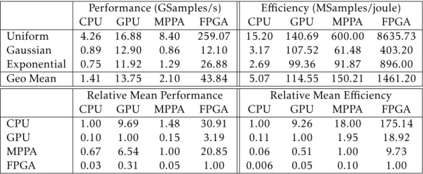
gener-ator across platforms. (Based on [43]) . . . 26 2.18 Processing Speed exact values for different image size and coding format [49]. 31 3.1 Processing Speed exact values for different image size and coding format [54]. 34 4.1 Decision Tree model parameters for Matlab Classification Learner. . . 40
5.1 Confusion Matrix for the Decision Tree Classifier . . . 52
5.2 Confusion Matrix for the Minimum Distance Classifier . . . 56
5.3 Decision Tree: Time to Perform Classification - Zynq board . . . 58
5.4 Decision Tree: Time to Perform Classification - I7 8750HQ 3.9GHz . . . 58
5.5 Minimum Distance: Time to Perform Classification - Zynq board . . . 59
I.1 Load_Init_Data block code . . . 71
I.2 DDR_Read_Controller . . . 75
I.3 DDR_Write_Controller . . . 78
I.4 Decision Tree Classifier Function . . . 81
AMBA Advanced Microcontroller Bus Architecture. ANN Artificial Neural Network.
ARM Advanced RISC Machines. AXI Advanced eXtensible Interface.
CC Correlation Coefficient.
CIE International Commission on Illumination. CNN Convolutional Neural Network.
COS Carta de Uso e Ocupação do Solo de Portugal Continental. CPU Central Processing Unit.
DMA Direct Memory Access. DT Decision Trees.
DUT Design Under Test.
DWT Discrete Wavelet Transform.
ESTARFM Enhanced Spatial and Temporal Adaptive Reflectance Fusion Model.
FF Fuzzy-Fusion.
FIMICA Fixed Identity Monotonic Identity Commutative Aggragation. FLAASH Fast Line-of-Sight Atmospheric Analysis of Spectral Hypercubes. FPGA Field-Programmable Gate Array.
GAN Generative Adversarial Network. GLCM Gray-Level Co-occurrence Matrix.
GPGPU General-Purpose Graphic Processing Unit. GPU Graphic Processing Unit.
IBM International Business Machines. IP Intellectual Property.
KNN K-Nearest Neighbors.
LiDAR Light Detection and Ranging. LUT Lookup Table.
MLC Maximum Likelihood Classifier. MPPA Massively Parallel Processor Arrays.
mtry number of variables in the random sampling.
NDSM Normalized Digital Surface Model. NIR Near Infrared.
NMSE Normalized Mean Square Error. ntree number of decision trees.
NVDI Normalized Difference Vegetation Index. OOB Out-of-Bag.
PL Programmable Logic. PS Processing System.
PSNR Peak Signal-to-Noise Ratio.
QUAC Quick Atmospheric Correction.
RGB Red, Green and Blue. ROI Region of Interest.
SAR Synthetic Aperture Radar. SDK Software Development Kit. SIMD Single Instructions Multiple Data. SoC System on a Chip.
STMRF Spatio-Temporal Markov Random Fields. SVM Support Vector Machine.
tiff Tagged Image File Format. UIQI Universal Image Quality Index.
VI Vegetation Index.
WFU Wildland Fire Use.
C
h
a
p
t
1
I n t r o d u c t i o n
This is an introductory chapter to contextualize the reader of the presented dissertation. In section 1.1 are presented context and motivation of the work being developed. In section 1.2 the problem being addressed with the proposed solution. At least, in section 1.3, a summary of the remaining chapters.
1.1
Context and Motivation
Fires have concerned the general public because of their highly presence in previous years, not just in Portugal, but in the rest of the world too. Their enormous devastation power destroys forests, cultivation lands and even buildings that become on their way. Even though all the effort by wildfire prevention programs, such as Wildland Fire Use (WFU), to control and put a stop into them, all the help from human and technology source is welcomed.
From the technology perspective, this dissertation pretends to implement a way to reduce the devastation power, minimize damages or prevent the start of a fire. The ap-proach will be a Land Use/Land Cover Classification technique to label the region of study into different classes. The results obtained can be further used in a fire sensor/al-gorithm to, for instance, a dry land where fires have higher chance to occur, to be cleared, or in case of an existing fire, to predict the direction where it may go. The Land Use/Land Cover Classification technique will be performed using spatial imagery.
Image processing has been a major interest among developers since its potentials in diverse areas, the most common being automatic reading of printed and handwritten text, high energy physics, cytology, medical diagnosis, analysis of biomedical images and signals, remote sensing, industrial applications, identification of human faces profiles, fingerprints and speech recognition, detection of resources from earth and automatic
classification of terrain [1]. This last topic mentioned, automatic classification of terrain, will be the main focus of the present dissertation.
In image processing there are two main problems that are commonly highlighted, the accuracy in decision making and the fast implementation [2]. It’s important to under-stand the trade-offs of each one and what is most crucial to the problem being approached. The fast response time became a requirement in the real-time system world, as systems became larger and more complex over time, with most usage in human and robot inter-action and imaging hardware [3]. In this case of study, it’s prioritized a higher reliability of the algorithms implemented, compromising the execution speed and response time. This decision is taken because the algorithms are intended to be accelerated in hardware platforms for the reasons that will be explained in chapter 2.
As mentioned before, image processing will be applied to terrain classification. Sev-eral studies have been made on this subject, which will be reviewed latter on. This theme has been intensely explored for its highly versatile applications. Humans use it for social-economic proposes in which the map generated by the system helps in the conservation planning of the location in analysis and in researching the intensity of human activity [4]. Also, the data extracted from the studies give a lot of support in "comprehension and analysis of natural phenomena such as climate change; provide a means to assess carbon stock accountability; and help monitor agriculture development, disaster management, land planning, defense of biodiversity, etc" [5].
To implement the algorithms required for image classification, several platforms can be used. Which one to choose depends on the approach been taken and what are the main system requirements. Also, it’s interesting to see, how a not so conventional plat-form, Field-Programmable Gate Array (FPGA), can present equivalent or better perfor-mance than other platforms such as Central Processing Unit (CPU) and Graphic Process-ing Unit (GPU).
In chapter 2 will be presented what methods are already being applied to Land Cover Classification, pros and cons of them and the comparison of different platforms to run the algorithms, such as CPU, GPU and FPGA.
1.2
Problem and Proposed Solution
This work will study the region of Sado estuary with the validation framework residing in itself. It’s the intention of future application for the classifiers to be applied in Mação, Santarém district. This choice is made due to Sado estuary regions allocate more diversity of Land Cover classes as well as more water information in Ocean, River Banks and Humid Regions. The scope of this work belongs to the project FORESTER, due to the forest fires of August, 2017, the region had a vast of its area burnt and land data for the village is no longer accurate.
The propose of this dissertation is to re-qualify and update the data using the above mentioned methods with further explanation in chapter 2. The goal is to implement
an algorithm able to correct qualify the land with the possibility to be used not just for the region of study but also in other scenarios. As mentioned, the results of this land classification have the intention to be used in future work to prevent a real fire scenario, before, during and after the event. The results should provide information about the area to cooperate in prevention, putting out and recovering.
The implementation will be performed in hardware because of its low power con-sumption and major capabilities in high processing imagery data. The classifiers to be run are Decision Tree and Minimum Distance. Due to their high accuracy and versatility (see 2.1.1), these algorithms should perform well in this context.
1.3
Outline
The following document is structured as follows:
Chapter 2 - Presents the algorithms already being used in Land Cover Classification with comparison between them with the scenarios where they are applied; also a comparison between platforms that are able to run such algorithms, first a more ab-stract point of view where the basic performance power of the platforms is analysed and then, a more contextualized approach for image classification; in the end, was chosen two algorithms, which will be implemented in the hardware, the literature reviewed has the objective to check the reliability of the implementation.
Chapter 3 - Describes the platform that will be used to develop the work; also the soft-wares required to support platform programming with the classifier. In the last section is presented the preprocessing operation done to the data so that it could be used in hardware.
Chapter 4 - In this chapter are described in detail the algorithms implemented for Land Use/Land Cover classification developed in software as well as in hardware. The two implementations are analyzed in detail with its correspondent models.
Chapter 5 - Presents the results obtained for the implementations. It compares the two classifiers performed in software and hardware in terms of performance time and accuracy.
Chapter 6 - This chapter concludes the work with what achievements have been made and future work to improve not just accuracy of the classifier but also the time to perform the classification.
C
h
a
p
t
2
S ta t e - o f -A rt
This chapter main focus is to present what methods and platforms are being used to help in Land Use/Land Cover Classification. Divided in three sections, first, in section 2.1, different methods and mathematical probabilistic systems are shown to accomplish the highest accuracy possible. As will be noticed, no algorithm is perfect and there are dif-ferent scenarios where one or another algorithm should be used, cause it presents better results for the case of study. Secondly, in section 2.2, a comparison of performance be-tween CPU, GPU and FPGA analysing the speed and processing power on them with special attention to image processing. And thirdly, in section 2.3, it’s discussed the possi-bility of implementing Land Use/Land Cover classification algorithms in hardware taking the benefits over software, what classifiers to implement and what platform will be used.
2.1
Land Use/Land Cover Classification
When considering Land Use/Land Cover Classification, it’s important to understand the effects of a good algorithm and the platform where it will be performed. How significant is the platform is described in more detail in section 2.2. This section focuses on what is considered a good algorithm. In subsection 2.1.1 are presented what algorithms are nowa-days being used in Land Use/Land Cover Classification and in subsection 2.1.2, some methodologies that improve land cover classification, such as removing environmental phenomena.
2.1.1 Classification Algorithms
For the problem being addressed, processing speed or accuracy should take more signifi-cance, rather than other factors, to accomplish the requirements of the system. Next will be presented several approaches in Land Use/Land Cover Classification, more specifically,
different algorithms. When considering an implementation of a classifier, it’s important to know if it will be a supervised or unsupervised classification. In supervised classifi-cation, the user has a training data set, in which pixel values/classes are known, then the computer algorithm labels the pixels to the class with highest probability of mem-bership [6, 7]. In unsupervised classification, no training data set is required, the user defines the number of classes that should be presented, and rules based on clustering algorithms group the data into the classes. Although this implementation is faster than the previous one, its normal accuracy is less than the supervised classification [7, 8]. The cross validation between the image classified and ground truth knowledge is usually made to calculate the accuracy. The most worldwide used spatial sensors to provide high resolution satellite imagery data are RapidEye, Worldview-2, GeoEye, GF-2 and Land-sat 8 [9, 10]. In table 2.1 are presented the supervised and unsupervised classification implementations, found in the reviewed literature, with a brief explanation of each one.
T able 2.1: Land C ov er Classifica tion Al g orithms studied in the liter ature review ed. Al g orithms Explana tion Supervised UNINORM The al g orithm im plemen ts a supervised system using an inf erence scheme, based on the rules applied, the output of each one represen ts the most likel y class to be assigned [11 ]. Decision Tree It ’s a tree-like model, buil t upon conditional sta temen t nodes, as deep as it is na vig ated in the tree, smaller subsets are found, the tree ends when the subsets are homog eneous [11 ]. Artificial Neur al Netw or k It learns by anal ysing exam ples in the tr aining da ta, the g oal is to detect pa tterns, based on pre-vious learning it classifies de v alida tion da ta sets [11 ]. Maxim um Likelihood Classifier The g oal is to find the par ameter tha t maximizes the likelihood function, in other w ords, in a sce-nario with more than one signa ture, it tries to assign the classifying object to the highest probabi-lity class [12 ]. Minim um Distance A distance is defined as an index of similarity so tha t the minim um distance is iden tified as the maxim um similarity [13 ]. Mahalanobis Distance The al g orithm assumes tha t the histogr am of the band has a normal distribution. It measures the distance betw een a poin t P and a distribution D, this distance is zero if P is at the mean of D and grows as P mov es aw ay from the mean [14 ]. K -Nearest Neighbor The al g orithm assigns the most common v al ue of the k nearest neighbors to the object being classified [15 ]. P ar allelepiped The al g orithm uses a sim ple decision rule, the decision boundaries form an n dimensional par al-lepiped classifica tion in the imag e da ta space. Based on threshol ds, the object is assigned to a class [16 ].
Support V ector Machine It ’s a non-probabilistic binary classifier , the g oal of this method is to find an hiperplane in an n dimensional space, dividing the ca teg ories with the widest g ap as possible [17 ]. Random Forest Is a meta estima tor tha t fits a n umber of decision tree classifiers on v arious sub sam ples of the 1 da ta set and uses av er aging to im prov e the predica tiv e [18 ]. Pixel-Based It ev al ua tes each individ ual pixel based on its spectr al inf orma tion [19 ]. Object -Based Groups the pixels tha t ha v e similar properties according to their spectr al properties [19 ]. Unsupervised K -Means Cl ustering It ’s objectiv e is to find k groups known a priori , the al g orithm focuses in minimize the cl ustering v ariability [20 ]. ISO Da ta The principle is the same as K -Means Cl ustering, but it all ows di ff eren t n umbers of cl usters to be g ener ated.
Like no photo and/or classification method is perfect, it can be also observed in the next literature reviewed, that to choose a land cover class, it is used the method with the smallest error or highest accuracy. To decrease the error, is also recommended the highest resolution image possible. Obviously it comes with a cost, so a resolution of 10 by 10 meters per pixel or less it’s good for classifying urban land objects, and a moderate reso-lution between 10x10m and 250x250m for pixel is suitable for Land Cover Classification [4].
For a more close look, in [21] it’s proposed the method of"fuzzy-fusion inference ap-proach for satellite image classification based on a fuzzy process". This method will be com-pared with Decision Trees (DT) and Artificial Neural Network (ANN) techniques in land cover classification for the district of Mandimba of the Niassa province, Mozambique. For this case scenario will be considered seven land cover classes summed up in table 2.2, and a classifier which uses five spectral bands, blue - band 1, green - band 2, red - band 3, Near Infrared (NIR) - band 4, Shortwave Infrared (SWIR) 2 - band 7, plus two indices Nor-malized Difference Vegetation Index (NVDI) and Vegetation Index (VI) 7.
Table 2.2: Classes used for Classification. (Based on: [21]) Class Name Class Description
Waterbody Areas covered by water (e.g. rivers, lakes) River Bancks Areas nearby water bodies
Bare Areas Areas without vegetation (e.g. rock outcrops) Croplands Areas covered by crops
Grasslands Areas covered by herbaceous vegetation Thickets & Shrublands Areas covered by shrubs (closed to open)
Forest & Woodlands Areas with a tree canopy cover greater than 10%
The fuzzy membership functions chosen for the test were an inductive method using histograms and fitted Gaussian functions, these allowed for a relative area to be classified based on the frequency of pixel values within a class. To demonstrate the errors that can occur when creating a membership function, in figure 2.1, is an example of a bimodality in an histogram, this is due to multiple classes been represented in a single pixel. Another type of error that can occur is, for instance, considering two classes, and performing the class membership to them, different bands can assign high values to different classes, leading to inconclusive results. To help in decision making, aggregation operators are used to give a positive or negative quotation to the classification: average, minimum, and two reinforcement ones, Fixed Identity Monotonic Identity Commutative Aggragation (FIMICA) and UNINORM. These two last ones (FIMICA and UNINORM) present better results in decision making, being UNINORM the best one with highest accuracy.
Applying the UNINORM to the area in study, and comparing with the two validation models, DT and ANN, it’s expected, with the proposed implementation, to obtain an accuracy close to those two. In table 2.3 can be observed what was hoped, being the overall accuracy not to disparate.
Figure 2.1: Example of a bimodal membership function, for band 1 [21].
Table 2.3: Accuracy of Classifying the training set using UNINORM, DT and ANN [21].
Water Body River Bank Bare Area Crop Land Grass Land Thickets & Shrublands Forests & Woodlands Total Average UNINORM 100.0% 91.1% 94.5% 97.6% 89.6% 90.7% 93.9% 93.9% DT 100.0% 100.0% 99.9% 95.1% 97.0% 91.1% 97.9% 97.2% ANN 98.2% 91.6% 100.0% 99.3% 97.4% 99.1% 97.3% 97.6%
Although ANN got a higher average validation accuracy for the training set, the out-come should be analysed in more detail, since Bare Areas had 100% accuracy not being true, cause as shown in table 2.4, acquired from the paper, it says the area to be validated had no Bare Areas, and in fact, it has. This justifies why the training set for the ANN has to be big enough so it can learn correctly. UNINORN and DT adapt better for small training sets.
Table 2.4: Percentage of class presence for the studied region using UNINORM, DT and ANN. (Based on: [21])
UNINORM DT ANN Water Body 3.1% 3.1% 3.2% River Bank 10.3% 13.9% 11.2% Bare Area 0.4% 0.6% 0.0% Crop Land 7.7% 6.6% 8.1% Grass Land 33.9% 26.4% 30.2%
Thickets & Shrublands 29.4% 35.0% 30.6% Forest & Woodlands 15.4% 14.5% 16.8%
Total 100.0% 100.0% 100.0%
The methodology presented in this paper has better results than DT and ANN when considering classification of Crop Land, also when considering River Banks, DT classi-fied them as Bare Areas in awkward regions, UNINORM did not present that kind of misleading. So, the approach had a good performance for the studied region.
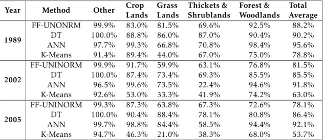
(1989, 2002, 2005) [11]. The aggregation operators, the five spectral bands and the two vegetation indices (rescaled to a normalized 8-bit unsigned [0,255] scale) to perform the analysis were kept from the paper [21]. Again seven classes are taken into consideration, but only five were used, merging Water Body with River Banks, and Bare Area with Croplands, for comparative results with [22]. The fuzzy membership functions were the same, histograms and Gaussian functions. An additional validation test was added for comparison, the K-Means clustering. The comparison of the tests is presented in table 2.5. It’s expected for the ANN approach to have a good accuracy, since the training set was good and wide. As mentioned before, ANN does not adapt as well to small training sets, as the other techniques do.
Table 2.5: Accuracy of classifying the training set with FF-UNINORM, DT, ANN and K-Means. (Based on: [11])
Year Method Other Crop
Lands Grass Lands Thickets & Shrublands Forest & Woodlands Total Average 1989 FF-UNONRM 99.9% 83.0% 81.5% 69.6% 92.5% 88.2% DT 100.0% 88.8% 86.0% 87.0% 90.4% 90.2% ANN 97.7% 99.3% 66.8% 70.8% 98.4% 95.6% K-Means 91.4% 89.4% 44.0% 67.0% 75.0% 78.8% 2002 FF-UNINORM 99.9% 91.7% 59.9% 63.1% 76.8% 81.5% DT 100.0% 87.4% 73.4% 69.3% 85.5% 85.5% ANN 96.5% 99.6% 73.5% 22.4% 94.6% 91.8% K-Means 92.6% 53.0% 33.3% 41.9% 74.2% 63.0% 2005 FF-UNINORM 99.3% 87.3% 63.8% 67.3% 72.6% 78.1% DT 100.0% 90.4% 88.4% 78.1% 80.8% 86.4% ANN 99.7% 98.8% 84.4% 58.5% 94.4% 92.1% K-Means 94.7% 46.3% 21.0% 38.3% 68.0% 53.7%
The ANN method presented the best results as expected, and more consistency ac-curacy throughout the years. In analyse to table 2.5, it’s noticeable that the Thickets & Shrublands class is the one where is harder to get a high correctness, might indicate a misclassified training set. Further tests presented in the paper showed that Fuzzy-Fusion (FF)-UNINORM and DT methods are the ones with most similarities and consistency when class attributing.
In the next case of study are used three other classification methods, Maximum Like-lihood Classifier (MLC), Mahalanobis Distance and Minimum Distance [12], explained before. The coverage area are the districts Klang, Petaling, Gombak and Hulu Langat of Selangor, and the land cover classes taken to test are Water Bodies, Forest, Agriculture, Urban and Open Land. The images used to perform the classification were acquired from Landsat 8 satellite and the ground truth was used to verify the identity of class types attributed to the images and build the overall accuracy of the algorithms. To fully understand the process, in figure 2.2 is shown the steps taken, since image acquisition till land cover classification.
Figure 2.2: Methodology Structure. (Based on: [12])
methods [23], and although Mahalanobis and Minimum Distances have a similar method-ology, differences shown in table 2.1, Minimum Distance algorithm is slower to classify the same data. In table 2.6 the advantage of using the Maximum Likelihood method with an overall accuracy of 88.88% compared to 74.44% and 78.88%, respectively Mahalanobis Distance and Minimum Distance. Producer Accuracy (PA) is related to the theoretical validation of the classifier and User Accuracy is related to the validation obtained from the case studied.
Table 2.6: Land Use and Land Cover classification efficiency of different methods [12].
Class Name
Techniques Maximum Likelihood Mahalanobis Distance Minimum Distance
PA (%) UA (%) PA (%) UA (%) PA (%) UA (%) Water Bodies 50.00 100.00 25.00 100.00 50.00 100.00 Forest 25.00 66.67 25.00 100.00 50.00 80.00 Agriculture 11.11 100.00 25.00 100.00 55.56 62.50 Urban 85.71 85.71 85.71 85.71 85.71 33.33 Open Land 87.50 31.82 87.50 26.92 25.00 100.00 Overall Classification Accuracy 88.88% 74.44% 78.88%
In a closer analyse, can be observed that the three different approaches, with a max accuracy difference of 10%, perform better for certain scenarios. For instance, having the MLC the highest accuracy, it shows clear difficulties when classifying Forest and Open Land. On the other hand, considering Minimum Distance with the interim result, it can classify well these two classes. At least, the Mahalanobis Distance, when classifying a terrain as Open Land, the results should be doubted cause the leak in accuracy showed in table 2.6. These results also agree with thek coefficient calculated in the paper, with Maximum Likelihood achieving 0.8216, Mahalanobis Distance - 0.6982 and Minimum Distance - 0.7893. Thek coefficient is used to measure how certain the algorithm will be able to identify the classes, using a statistical method for qualitative rating, it takes into consideration agreements occurring by chance [24]. Ak coefficient close to 1 means the method has a high reliability, conversely, ak coefficient closer to 0 has poor accuracy and
should not be used as its doubtful classification.
Deeper analysis to the Minimum Distance Classifier, in [13], a different approach with Discrete Wavelet Transform (DWT) is presented, and as it will be seen, an improve-ment in the classification accuracy is made. A DWT decomposes the image in its fre-quency spectrum, in this case, up to eight levels. A wavelet is an oscillation, in which amplitude begins in zero, increases and decreases, returning in the end back to zero. A DWT is a discrete time signal obtained by sampling a continuous translation and scale parameter of a wavelet [25], also it is characterized by its components, the high and low frequency are detail and approximation coefficients, respectively. In this study, the de-composition method is Haar wavelet, which turns the wavelet into a square shape form taking the values 1 for 0 ≤ t <1/2, -1 for1/2≤t < 1 and 0 for other values of t.
The performance tests were run to a five class classification, Urban, Fallow Land, Water, Vegetation and Agriculture and eight levels of image decomposition. The accu-racy table is presented in table 2.7. To overcome the issues derived from atmospheric imperfections, an atmospheric correction method was implemented, Quick Atmospheric Correction (QUAC). It uses the information in the image/scene, visible and near infrared and shortwave infrared spectrum to adjust the compensation parameters to clear up the image [26].
Table 2.7: Overall Accuracy for wavelet decomposition levels with Minimum Distance approach [13]. Wavelet Decomposition Level Overall Accuracy (%) 1 75.2693 2 85.9600 3 88.8737 4 93.4666 5 95.0346 6 93.0087 7 92.3187 8 90.8021
The fifth level of decomposition, with 95.0346% of accuracy, had the highest score. Also to be noticed is that, the first level has approximately the same result as [12], due to equivalent implementations. The first level implements the method for the original image, without any decomposition, this being said, the only difference between the two papers is the region of study. The DWT presents a 20% increase in the overall accuracy, allowing the method some reliability and the possibility to be executed in other scenarios, situation that had no chance before, because there was no trust in the classification.
As mentioned before, moderate and high resolution Earth imagery for Land Cover Classification comes with their inherent costs. In [4], the data is provided by Google Earth, a free program owned by Google Inc. with a sub-meter pixel resolution, other satellite images can be paid. The region of study is the city of Bangalore, India and
the land classes to be defined are Water Body, Building, Vegetation, Road Network and Bare Land. The method to perform this classification and after, comparison of results, is K-Nearest Neighbors (KNN) with Euclidean Distance and Average Pixel Intensity as parameters when choosing labeling. Not just the Red, Green and Blue (RGB) colors were used to identify the classes, but they were converted intoLab. Lab was defined in 1976, by the International Commission on Illumination (CIE) as a color space [27]. Its purpose was to convert from a three channel RGB into lightness-L, green/red-a and blue/yellow-b. This way, in the scenario of [4], the illumination between objects could be identified and a easier and more accurate analysis made.
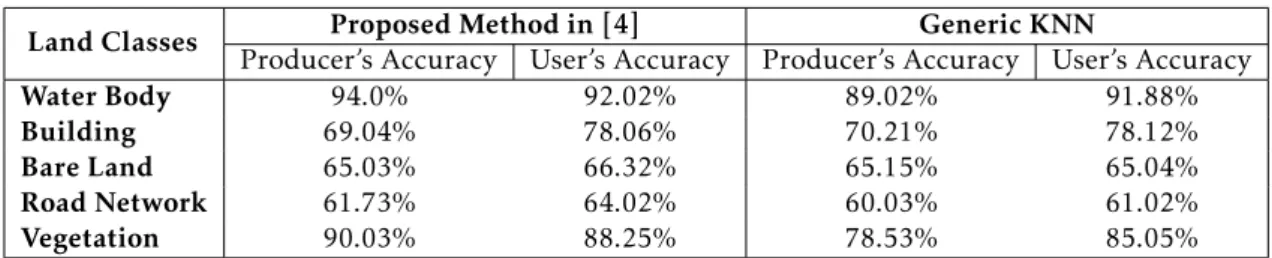
It’s pretended to see what is the improvement of a generic KNN method to a Euclidean Distance and Average Pixel Density based one. The accuracy results for the studied region are presented in table 2.8.
Table 2.8: User’s and Producer’s Accuracy values of Generic KNN and Euclidean Distance and Average Pixel Density based KNN. (Based on: [4])
Land Classes Proposed Method in [4] Generic KNN
Producer’s Accuracy User’s Accuracy Producer’s Accuracy User’s Accuracy
Water Body 94.0% 92.02% 89.02% 91.88%
Building 69.04% 78.06% 70.21% 78.12%
Bare Land 65.03% 66.32% 65.15% 65.04%
Road Network 61.73% 64.02% 60.03% 61.02%
Vegetation 90.03% 88.25% 78.53% 85.05%
As seen in the result table, the overall accuracy went from an average of 75.04% in the Generic KNN to 76.38% in the proposed method. The reason for the improvement is, instead of using only one parameter for class labeling, the presented method uses two, Euclidean Distance and Average Pixel Density. Furthermore, the Generic KNN imple-mentation had misclassifications with waves of water body and some part of vegetation, labeling them, respectively, buildings and road network. The method also helped to solve the problem.
Another classifier is the Random Forest. How it performs can be observed in [28] were it was put the test in a six class Land Cover Classification scenario, in Xuchang city, Henan Province, China. The data provided by the GF-2 satellite and an airborne Light Detection and Ranging (LiDAR) was used together for accuracy improvement. GF-2 providing spectral features and texture information and LiDAR the three-dimensional coordinates. To generate seven scenarios to test the effectiveness of the classifier, NVDI, Normalized Digital Surface Model (NDSM) and Gray-Level Co-occurrence Matrix (GLCM) texture were used with different combinations of the input variables, described in more detail in table 2.9.
To properly function, the Random Forest classifier requires two parameters, the num-ber of variables in the random sampling (mtry) used at each split to grow a decision tree and the number of decision trees (ntree). To optimize the parameters the Out-of-Bag (OOB) error grid search approach was used. The OOB is a method applied not just to
Table 2.9: Different Scenarios and Input Variables. (Based on: [28]) Input Variables
Scenario 1 4 variables generated by the GF-2 (red, green, blue and near-infrared) Scenario 2 5 variables generated by the GF-2 and NDVI
Scenario 3 85 variables generated by the GF-2, the NDVI and their texture features (7x7 and 9x9 pixels)
Scenario 4 1 variable generated by the NDSM
Scenario 5 17 variables generated by the NDSM and its texture features (7x7 and 9x9 pixels)
Scenario 6 6 variables generated by the GF-2, NDVI and NDSM
Scenario 7 102 variables generated by the GF-2, NDVI, NDSM and their texture features (7x7 and 9x9 pixels)
Random Forest but also to boost decision trees and other machine learning approaches, and it measures the estimated test error of the bag, this way it’s possible to estimate the error in a node [breiman1996out, 29].
To fully optimize the accuracy in every scenario, it was used the mtry and ntree parameters. When the value of the OOB error is low, it indicates a good reliability of the model. The accuracy results for the seven scenarios are presented in table 2.10, where can be observed that, seventh scenario had the best accuracy with 93.32% and kappa value of 0.91.
In analysis of the results, can also be seen, that the fourth scenario presents poor results and should not be used. Again, a confrontation between accuracy and kappa values, they vary proportionally to each other. In further detail, the easiest class to be identified was the Cropland, since for all scenarios and producer’s and user’s accuracy it scored 100% accuracy.
Table 2.10: Total Accuracy and Kappa Coefficient for all Scenarios [28]. Scenario Total Accuracy (%) Kappa Coefficient
1 76.86 0.70 2 77.11 0.71 3 83.33 0.79 4 57.59 0.44 5 80.13 0.74 6 89.97 0.87 7 93.32 0.91
As mentioned, satellite imagery might have a lot of noise, including granularity and clouds, blocking the possibility to implement a method that can perform a Land Use/-Land Cover Classification for the studied region. To overcome this problem, in [30], it’s
used a spatial-temporal fusion technique. This is based on acquiring images from dif-ferent sensors and/or at difdif-ferent times and grouping the data. The fusion model used is Enhanced Spatial and Temporal Adaptive Reflectance Fusion Model (ESTARFM) which compounds Landsat 8 and MODIS data. To extract the information from the imagery and identify the classes, an object-based strategy is used. An object-based classification not just considers and analysis the pixel itself but the surrounding ones too, this combines image segmentation with knowledge-based classification. Image segmentation decreases the complexity and divides the image into regions, when these become meaningful, they are considered image objects [31]. According to [32] an object-based approach is able to achieve higher accuracy than a pixel-based approach. In the paper, the technique used was provided by the platform eCognition9.0 and"the algorithm is a region growing tech-nique that starts with a pixel forming an object and merging the neighbouring pixels until the homogeneity criterion is achieved".
The data used in this paper was acquired from the Landsat 8 and MODIS sensors. The Landsat 8 OLI imagery acquired three times in the year 2015, had a cloud coverage less than 1% and a higher resolution than the one from the MODIS sensor. On the other hand, MODIS imagery (including Red and NIR bands) was acquired with a time span of 8 days during the year 2015. The fusion of these two helped to remove the effects of atmospheric interference by correlation of the combined data. The major problem was the poor resolution of 250m per pixel. As for the training and posterior validation sets, the data used was from the GF-1 with a resolution of 2m per pixel (2015-09-15) and Google Earth (2015-09-08). In diagram shown in figure 2.3 is a demonstration how the time series imagery was created with MODIS and Landsat 8 data sets.
Figure 2.3: Flowchart of the fusion data sets [30].
The studied area was Changsha City, China and the main focus classification tech-nique was an object-based method, as above explained, with fused Landsat 8 time series.
Also taken to test and comparison, other three techniques were performed, an object-based method with OLI images, an object-object-based method with single date Landsat 8 image and a pixel-based method with Landsat 8 data set. To verify the accuracy of the tests, a confusion matrix with ground truth reference data of the studied region was made. A summary of the training and validation samples for the Region of Interest (ROI) with the different classes is presented in table 2.11.
Table 2.11: Number of ROIs and Pixels for different classes in training and validation data sets [30].
Number of ROI
and Pixels Water Grassland
Cultivated Land
Dry
Land Forest Building Barren
Training Samples Number of ROIs 196 102 124 95 202 113 92 Number of Pixels 3256 4585 2168 3749 4053 3821 2897 Validation Samples Number of ROIs 48 52 58 69 83 52 71 Number of Pixels 1048 1204 850 1426 1987 967 1436
It’s expected for the classes with highest number of training samples, to achieve better accuracy. This is not always linear, as different classes have lower/higher degrees of com-plexity in classification methods; other factors, for instance over-fitting, can introduce errors in the validation test, for not being a classifier able to general use, cause it adapts and memorizes the training samples and do not learn the method for a correct classifica-tion. A comparison will be made after the analyse of the accuracy result table 2.12. Table 2.12: Classification Accuracy Comparison with different training data sets and methods. (Based on: [30])
(a) Landsat 8 data sets and object-based method Cover Types Producer Accuracy % User Accuracy % Total Classification Accuracy % Water 97.25 97.12 94.38 Grass Land 86.84 85.69 Cultivated Land 88.72 87.26 Dry Land 89.23 88.15 Forest 92.64 93.52 Building 96.38 95.41 Barren 92.69 91.83
(b) Landsat 8 OLI images and object-based method Cover Types Producer Accuracy % User Accuracy % Total Classification Accuracy % Water 95.82 95.02 90.65 Grass Land 83.53 82.32 Cultivated Land 85.68 85.09 Dry Land 84.62 82.73 Forest 90.52 90.18 Building 96.35 95.41 Barren 92.68 91.83
(c) Single Landsat 8 image and object-based method Cover Types Producer Accuracy % User Accuracy % Total Classification Accuracy % Water 96.13 95.24 86.52 Grass Land 78.25 76.28 Cultivated Land 75.59 77.36 Dry Land 79.15 78.47 Forest 88.49 88.46 Building 94.23 93.82 Barren 90.63 89.58
(d) Landsat 8 data sets and pixel-based method Cover Types Producer Accuracy % User Accuracy % Total Classification Accuracy % Water 96.68 96.31 88.62 Grass Land 82.26 81.35 Cultivated Land 83.82 82.69 Dry Land 85.23 84.56 Forest 89.81 90.45 Building 95.64 94.18 Barren 91.59 90.27
The approach presented in the paper, the object-based method with fusion time series imagery, had the highest accuracy of the four tests, proving that the implementation
and the training data sets are two big factors in image classification, moreover in Land Cover Classification. When used the same data set, in sub tables 2.12a and 2.12d, it’s possible to see the main difference between implementations, object-based and pixel-based, respectively. Considering the pixel itself and the surrounding information, more features can be extracted from the image, leading to a more accurate analysis. For sub tables 2.12a, 2.12b and 2.12c, that used the same method, it’s compared the importance of a good training data set. From the data set obtained by the fusion of images explain in figure 2.3, to the three images acquired from the Landsat 8 OLI and finally to a single one also from Landsat 8, it’s clearly seen the difference in accuracy, through the output results.
In consideration to the accuracy results for the individual classes, regardless of the implementation, it’s important to notice the influence of enough training samples. The classes with more training samples are Water, Cultivated Land, Forest and Building, and in general, Water had the best accuracy. In contrast, Cultivated Land didn’t had a good accuracy as foreseen, this is due its misclassification as Grass Land and Dry Land to their similar features.
Some improvements to increase the accuracy are, even better data sets to have a cloud free imagery and reduce the uncertainty of the ESTARFM fusion model images. A high resolution imagery would also help to solve the problem of misclassification. When small regions are attributed with the wrong class by the object-based method, a combination with spectral mixture analyses would improve the results.
The previous cases of study showed Land Cover Classification based on supervised methods, except for [11] which briefly presents K-Means clustering. The next paper explores in more detail unsupervised classification, with ISO-Data and K-Means imple-mentations, also with other two new supervised methods, Parallelepiped and Support Vector Machine (SVM). In [7] are presented four supervised classification methods, Max-imum Likelihood, MinMax-imum Distance, Parallelepiped and SVM and two unsupervised, ISO Data and K-Means. From the above mentioned studies, the classification method expected to obtain the highest accuracy was the Maximum Likelihood. The scenario to perform these tests is Paonta Sahib, Himachal Pradesh, India. Since unsupervised algo-rithms depend on their rule set for the classification, the accuracy they’re able to achieve is less than supervised ones which use training data sets in their approach, being much more flexible for different scenarios. For the Paonta Sahib region were defined seven land classes, River, Forest, Urban, Mountain, Scrub Land, Crop Land and River Associated Sand and for the supervised classifiers, the training data sets were restricted to thirty samples per class. The training data set imagery was acquired from Sentinel 2A and its resolution depends on the bands, varying between 10x10m and 60x60m per pixel. After a process of stacking, the final resolution was 10x10m per pixel. The final classification of the different implementations were compared to a ground truth data, and by a confusion matrix, the accuracy results obtained are presented in table 2.13.
Table 2.13: Accuracy measurements of supervised and unsupervised classification meth-ods. (Based on: [7])
Method Accuracy (%) Kappa Coefficient Supervised Maximum Likelihood 89.30 0.8481 Minimum Distance 61.90 0.5031 Parallelepiped 80.07 0.7054 SVM 75.58 0.6546 Unsupervised ISO Data 30.03 0.0917 K-Means 22.09 0.0917
by Parallelepiped, SVM and Minimum Distance. The worst two were the unsupervised methods, as it was anticipated. Between them, the best one with 30.03% is the ISO Data. In relation with [12], where also the Maximum Likelihood Classifier was putted to the test, the outcome is really close to which other, proving the consistence of the algorithm. For a context where no previous imagery of the region is available, and an unsupervised method is the only way to proceed, the results are doubtful as poor accuracy was obtained.
From paper [7], SVM had a poor accuracy and an aforementioned methodology pixel-based to object-pixel-based approach seemed to increased the accuracy from the pixel-pixel-based im-plementation. It’s in the interest of [10], to combine MLC and SVM classifiers with pixel and object-based strategy to perceive how they work together and the benefits they bring to the context. Therefore, for the region of Shandong Province, China were applied four classifications approaches, pixel-based with MLC, pixel-based with SVM, object-based with MLC and object-based with SVM. The imagery data was acquired (two adjacent scenes) from the spatial sensor GF-2 in 2016 with a resolution of 4m per pixel and a cloud free coverage, even though, an atmospheric correction was applied, the Fast Line-of-Sight Atmospheric Analysis of Spectral Hypercubes (FLAASH), to fully optimize the process. For the area addressed were defined five classes, winter wheat, woodland, water, vegeta-bles and artificial surfaces that covers construction, roads and residential areas. These classes were chosen because agriculture is very important for the region and knowing the conditions of the terrain helps farming.
From the imagery data, were selected random pixels, with the help of ENVI version 5.0 software, to constitute the training data set. The total number of pixels used for training are 2,741 pixels for winter wheat, 4,780 pixels for woodland, 27,162 pixels for water, 11,816 pixels for artificial surfaces and 3,472 pixels for vegetation.
When performing the object-based, it’s used segmentation to clear separate the objects identified. Different scales of segmentation can be applied, in the paper was studied a
variation between 10 and 100 levels with the optimum found to be 25. Table 2.14 presents the results for the four tests.
Table 2.14: Land Cover Classification with Pixel and Object-Based strategies and MLC and SVM classifiers. (Based on: [10])
Pixel-Based MLC Pixel-Based SVM Object-Based MLC Object-Based SVM PA (%) UA (%) PA (%) UA (%) PA (%) UA (%) PA (%) UA (%) Winter Wheat 86.54 83.00 89.16 82.23 85.99 82.85 93.43 85.48 Woodland 83.74 92.86 97.20 84.37 91.05 95.96 99.33 94.77 Water 87.18 97.70 88.32 98.75 91.75 99.32 94.58 98.73 Artificial Surface 87.34 74.61 89.76 79.50 94.47 83.79 94.13 89.74 Vegetables 84.45 61.95 84.71 76.21 85.37 70.99 86.90 84.91 Overall Accuracy 86.67 89.30 91.57 94.33
Kappa Coefficient 0.796 0.836 0.870 0.911
Although MLC was expected to present the highest classification accuracy [33], SVM had 94.33% for the object-based strategy. In analyse to table data, Water class is correctly identified in all four approaches. Also an improvement is noticeable between a pixel-based strategy and a object-pixel-based one, being the major difference in the Artificial Surface, with an almost 10% accuracy increase for both scenarios. SVM also had fewer misclas-sifications between Woodland and Vegetables. More detailed review, reviled that SVM performed better than MLC in regions with small area, and with the high resolution sen-sor used, this difference is nearly 3%. From [7], where the resolution was 10x10m per pixel, a better resolution demonstrates that other classifier should be used due to highest accuracy achievements.
In table 2.15 is summed up the cases of study with the classifiers they use in their approaches, with easy access to what classifiers are research in each study and for a specif classification technique, what studies approach it.
T able 2.15: Summary of cases of study and their im plemen ted classifiers. Al g orithms Applied/ C ases of S tudy UNINORM DT ANN ML C Min Dist Mah Dist KNN P ar al SVM RF PB OB K -Means ISO-Da ta [21 ] [11 ] [12 ] [13 ] [4 ] [28 ] [30 ] [7 ] [10 ]
2.1.2 Cloud Free Imagery
When considering satellite imagery, one of the biggest concerns is to remove the imperfec-tions, mainly caused by atmospheric phenomena, namely clouds and fog. According to [34] there are three major implementations for cloud removal, spatial interpolation based, multi spectral based and multi temporal based. Spatial interpolation based approach uses the non cloud parts of the image to reconstruct the affected areas but with low accuracy results, the multi spectral based approach restore the image using different bands of the spectrum but it is restricted by thick clouds, the multi temporal based approach fuses images from different dates to use the good parts of each one, the only trouble being the time consumption. Previously was mentioned the QUAC approach which uses the band spectrum to correct the parameters and tries to clean the image. Also a time se-ries implementation can be used, having different time imagery for the same region and the correlation of data is made and eliminate the affected areas. The following litera-ture introduces several implementation where the goal is to achieve a cloud free satellite image.
In cloud removing procedure, it can be challenging to distinguish what is actually clouds or cloud-shadow from just bright areas. Even though thresholds can solve the problem when the difference is noticeable, rarely this happens. To overcome this issue, in [35] is implemented a mosaicking approach, with cloudy images acquired from IKONOS and SPOT satellites. The images from the satellite sensors had the influence of different atmospheric conditions and to correctly perform the mosaicking process it required that they become the most similarly possible, this means, if the brightness levels are disparate throughout the images, a gray balance is made to standardize it.
During the process, the classes taken to consideration were Clouds, Vegetation, Build-ings and Bare Soil and some of the Bare Soil areas were wrongly labeled as Clouds. To solve this, a different criteria was applied, a three threshold determined from the his-togram is made, Shadow Intensity, Cloud and Vegetation Intensity. Then, for the non affected pixels, they were again classified as Vegetation, Open Land and other. Briefly, the pixels are classified as problematic and non problematic, the non problematic ones are then classified as Vegetation, Open Land or other, and the problematic ones are clas-sified as Clouds or Shadows. At this point, the images will be merged. If a pixel was labeled with the Vegetation class for one image, can be assumed for the other images where doubtful classification was made that the pixel belongs to the Vegetation class avoiding discontinuity.
An other implementation of cloud removal depicted in [36], shows an algorithm that only uses visible bands of the frequency spectrum. The proposed method is Generative Adversarial Network (GAN). GAN is an artificial intelligence algorithm that uses two networks, one to generate fake images, which are almost look a like the originals and the second one, evaluate the previous one [37]. The original application of GAN, used visible and invisible bands, yet, the paper’s method restricts itself to the visible ones. This
2 . 1 . L A N D U S E / L A N D C O V E R C L A S S I F I C AT I O N
implementation was taken as the region of study (Paris) is very cloudy and clouds have high reflectance on NIR band.
The data set training from GAN was derived from Sentinel 2 satellite sensor, compris-ing twenty cloudy (10 to 100% cloud coverage) images and thirteen cloudless (0 to 5% cloud coverage). For the initial weights of the learning process of the neural network, a Gaussian distribution was done. As for the region of study, no complete cloud free im-agery is available, no real scenario test could be analysed. To check de reliability of GAN approach a simulated context was made. Taken the imagery available, a Perlin noise was added to the cloud free images, which has the visual appearance of clouds. A sum-mary of the five tested images is in graphic of figure 2.4 with Peak Signal-to-Noise Ratio (PSNR) results, where high result is better, meaning greater relation between cloudless and cloudy area.
3.1. Dataset
Our dataset is composed of high resolution Level-1C Sentinel-2 imagery ranging between the year Sentinel-2015 till Sentinel-2017. Sentinel-Sentinel-2 is a multi-spectral dataset, with each spectral band is stored as a separate image [12]. For our experiments, we choose images only from visible bands i.e. Blue (B2), Green (B3), Red (B4) all of which have 10 meters of spatial resolution.
Most of our cloud-free images are selected with 0-5% cover while for cloudy images we chose range anywhere be-tween 10 to 100. All the images are downloaded over the Paris region as it is easy to get quite a range of cloudy images. We choose 20 cloudy and 13 cloudless images for training. We then extract 512 × 512 patches from these images. After filtering of unwanted ones, a total of 1677 patches for each cloud and cloud-free dataset were extracted while for testing we had 837 patches. For computational efficiency in training, we resize them to 256 × 256.
3.2. Network Architectures
We imbibe the architecture and the naming convention sim-ilar to what have been used by [10]. Generator architecture, uses 6 blocks for 128 × 128 training images and 9 blocks for 256 × 256 or higher resolution images. Additionally, a re-flection pad is imbibed to avoid artifacts. The Discriminator architecture consists of a 70 × 70 PatchGAN [8], classifying 70 × 70 patches as real or fake data. Thus, it can effectively be applied to any input size image and has lesser number of parameters.
3.3. Training
Initialization of weights was done through a Gaussian distri-bution with mean 0 and standard deviation 0.02. Optimiza-tion was carried out using ADAM [13], with a batch size of 1 and λ = 10 for all experiments. We perform training from scratch using a learning rate of 0.0002 up-to 200 epochs. The learning rate was kept constant for the first 100 epochs after which it linearly decays to zero until the last epoch. Also, as illustrated in [10] model oscillations are avoided by using a history of generated images (50) rather than only one.
4. RESULTS AND DISCUSSIONS
We present the results obtained using Cloud-GAN in Figure 3 (for real clouds) and 4 (for synthetic clouds). Without using any corresponding Cloud-Free pair for a cloudy image, our Cloud-GAN efficiently removes thin clouds spread through-out a scene, as shown in row III, IV, V in Figure 3. More interestingly, it effectively detects small cloudy patches and replaces them with the underlying ground details, as depicted in row I and II in Figure 3. Cloud-GAN interestingly is able
Fig. 4:Sample images from Synthetic dataset where (a) Scene-5 (b) Scene-4
to retain finer details like patches of urban settlements, river, fields (row IV) while getting rid of the cloudy film. In some cases e.g., row II, the generated image from our method is more natural and visually more pleasing than the original im-age which is a byproduct of our method.
We cannot report any quantitative results on the real dataset since we lack paired cloudy-cloud-free images. How-ever, to compensate for that, we report results on 5 synthetic scenes, composed by addition of Perlin noise to cloud free images. We provide the corresponding PSNR results in Fig-ure 5. We observe that even though we trained our model on real dataset, our model substantially outperforms on all synthetic scenes by a significant margin. Figure 4 shows two of these test scenes. Note that we do not provide comparison with [9], due to the unavailability of their code and dataset.
We additionally show some special instances of thick cloud (Figure 6) where our model fails to yield credible re-sults. In Figure 6 row I, we see that the model contends by generating an over-smoothed image when the clouds are too opaque. In Figure 6 row II, the model fails completely to produce an image as the clouds have occupied most of the visible area. One of the reasons can be that the network finds no closest sample in the target dataset and hence predicts a spatially smooth region under the cloud or some random noise. The only way to solve this is by the addition of an ex-tra source such as SAR images which can peneex-trate through these clouds and give us details of the underlying ground details.
Scene-1 Scene-2 Scene-3 Scene-4 Scene-5 22 24 26 28 PSNR (dB)
Cloudy Cloud Free
Fig. 5: Quantitative results on Synthetic Scenes
5. CONCLUSIONS
We have proposed a novel technique to remove thin clouds
from Sentinel-2 imagery. Our cloud removal technique
Figure 2.4: PSNR for simulated scenarios with GAN [36].
The cloud free imagery, after GAN been run, has more than 4dB in the relation treated and original images, proving the efficiency of the method. The application of GAN with only visible band usage has its limitations, for an image with significant cloud coverage, the result can be an over smoothed image or a complete fail performance.
A more detailed analyse to the three aforementioned approaches is presented in [34]. It studied the difference between results of the implementations and proposes a comple-mentary multi source methodology to be added into multi temporal. When considering multi temporal image fusion, it’s convenient that the imagery data acquired is done in the shortest time possible, so the land coverage do not suffers changes. As high resolution satellite images acquisition has limited periodicity, multi source will be performed and final results discussed. The multi source data derive from a low resolution spatial sensor but with much higher frequency of image acquirement.
The concept behind this is, in a high resolution image, if there is an affected area by means of a cloud, the images acquired from the lower resolution sensor with closest date and that do not present irregularities in that area, are used to cover the specified region. The high resolution images were acquired from Landsat satellite sensor and the low resolution ones from MODIS. To represent the three implementations, Poisson, Weighted Linear Regression (WLR) and Spatio-Temporal Markov Random Fields (STMRF) methods were used and compared with the purposed one. Two tests were performed, both cloud simulated, the second one presenting a more fragmented scenario. The parameters to
observe the quality of the methods when reconstructing a scene are Normalized Mean Square Error (NMSE) where low results are better, as for Correlation Coefficient (CC) and Universal Image Quality Index (UIQI) higher is better. The final results are shown in table 2.16.
Table 2.16: Results for Spatial Resolution, Multi Spectral, Multi Temporal and Spatiotem-poral approaches in cloud removal operation [34].
Poisson WLR STMRF Proposed in [34] Test 1 CC 0.6662 0.7177 0.6946 0.8411 NMSE 0.0505 0.0434 0.0616 0.0260 UIQI 0.6268 0.7107 0.6909 0.8135 Test 2 CC 0.3894 0.6689 0.5861 0.5780 NMSE 0.6852 0.0670 0.0900 0.0938 UIQI 0.3404 0.6610 0.5682 0.4939
For the first test, the proposed method had the best results in every parameter taken to consideration, although, for the second test, neither STMRF or the proposed method score higher than WLR. This is majorly due to spectral mixed pixels from the MODIS sensor and radiometric inconsistency between Landsat and MODIS sensors.
2.2
FPGA vs CPU vs GPU
As mentioned, when discussing image processing, it’s important to understand two main standards, the speed of data processing and accuracy in decision making. There are also other effects that should be taking in consideration such as energy consumption, cost, size, reconfigurability, application-design complexity and fault tolerance. All these have implementation trade-offs and what it’s most required for the system being implemented must take higher priority.
Since the demand of greater and more complex problems have reached society, the need of powerful machines and high performance processing units is a must. To achieve a high performance either the operational frequency is very high or the architecture is implemented with parallelism. Systems have changed from a sequential processing approach to a parallel programming one [38], this can be observed in the past years, where the trend of parallelism architectures has increased over time [39].
Different platforms can be used to run the algorithms implemented, here it will be considered CPU, GPU and FPGA. Several studies have been made to compare the perfor-mance of these three. As shown in [40], the right balance between operational frequency and parallelism may lead to an optimal performance.
Till a few years ago, programmers have rely in fast and powerful processors, with high clock frequency, which enables a software application to run smoothly and with no ap-parently latency. This wasn’t an issue when these applications didn’t take full advantage
![Table 2.3: Accuracy of Classifying the training set using UNINORM, DT and ANN [21].](https://thumb-eu.123doks.com/thumbv2/123dok_br/15224254.1020913/34.892.159.786.481.575/table-accuracy-classifying-training-set-using-uninorm-ann.webp)
![Table 2.6: Land Use and Land Cover classification e ffi ciency of di ff erent methods [12].](https://thumb-eu.123doks.com/thumbv2/123dok_br/15224254.1020913/36.892.150.789.660.840/table-land-land-cover-classification-ciency-erent-methods.webp)
![Table 2.9: Di ff erent Scenarios and Input Variables. (Based on: [28]) Input Variables](https://thumb-eu.123doks.com/thumbv2/123dok_br/15224254.1020913/39.892.226.625.886.1065/table-erent-scenarios-input-variables-based-input-variables.webp)
![Figure 2.3: Flowchart of the fusion data sets [30].](https://thumb-eu.123doks.com/thumbv2/123dok_br/15224254.1020913/40.892.248.680.745.1042/figure-flowchart-fusion-data-sets.webp)
![Table 2.16: Results for Spatial Resolution, Multi Spectral, Multi Temporal and Spatiotem- Spatiotem-poral approaches in cloud removal operation [34].](https://thumb-eu.123doks.com/thumbv2/123dok_br/15224254.1020913/48.892.219.711.319.468/results-resolution-spectral-temporal-spatiotem-spatiotem-approaches-operation.webp)