potential evapotranspiration ratio as determined by
the global eddy flux measurements
Chunwei Liu1, Ge Sun2, Steven G. McNulty2, Asko Noormets3, and Yuan Fang3
1Jiangsu Provincial Key Laboratory of Agricultural Meteorology, College of Applied Meteorology,
Nanjing University of Information Science and Technology, Nanjing 210044, China
2Eastern Forest Environmental Threat Assessment Center, Southern Research Station, USDA Forest Service,
Raleigh, NC 27606, USA
3Department of Forestry and Environmental Resources, North Carolina State University, Raleigh, NC 27695, USA
Correspondence to:Ge Sun ([email protected])
Received: 15 May 2016 – Published in Hydrol. Earth Syst. Sci. Discuss.: 24 May 2016 Revised: 27 December 2016 – Accepted: 28 December 2016 – Published: 18 January 2017
Abstract.The evapotranspiration/potential evapotranspira-tion (AET/PET) ratio is traditionally termed as the crop coefficient (Kc) and has been generally used as ecosystem evaporative stress index. In the current hydrology literature,
Kchas been widely used as a parameter to estimate crop wa-ter demand by wawa-ter managers but has not been well ex-amined for other types of ecosystems such as forests and other perennial vegetation. Understanding the seasonal dy-namics of this variable for all ecosystems is important for projecting the ecohydrological responses to climate change and accurately quantifying water use at watershed to global scales. This study aimed at deriving monthlyKc for
multi-ple vegetation cover types and understanding its environmen-tal controls by analyzing the accumulated global eddy flux (FLUXNET) data. We examined monthlyKcdata for seven
vegetation covers, including open shrubland (OS), cropland (CRO), grassland (GRA), deciduous broad leaf forest (DBF), evergreen needle leaf forest (ENF), evergreen broad leaf for-est (EBF), and mixed forfor-est (MF), across 81 sites. We found that, except for evergreen forests (EBF and ENF), Kc val-ues had large seasonal variation across all land covers. The spatial variability ofKcwas well explained by latitude,
sug-gesting site factors are a major control on Kc. Seasonally, Kc increased significantly with precipitation in the summer
months, except in EBF. Moreover, leaf area index (LAI) sig-nificantly influenced monthlyKcin all land covers, except in
EBF. During the peak growing season, forests had the
high-estKc values, while croplands (CRO) had the lowest. We developed a series of multivariate linear monthly regression models forKcby land cover type and season using LAI, site latitude, and monthly precipitation as independent variables. TheKc models are useful for understanding water stress in different ecosystems under climate change and variability as well as for estimating seasonal ET for large areas with mixed land covers.
1 Introduction
The ratio of AET to PET is traditionally termed as crop coefficient (Kc), and has been widely used to as a
parame-ter to estimate crop waparame-ter demand by waparame-ter managers (Allen and Pereira, 2009; Irmak et al., 2013a). However, this pa-rameter has not been well examined for other ecosystems (Zhou et al., 2010; Zhang et al., 2012). The ratio of AET to PET has also been used as an indicator of regional terres-trial water availability, wetness or drought index, and plant water stress (Anderson et al., 2012; Mu et al., 2012). When the annual AET/PET ratio is close to 1.0, the soil water meets ecosystem water use demand. The ratio of AET/PET or water stress level can be drastically different among dif-ferent ecosystems in difdif-ferent environmental conditions, be-cause AET is mainly controlled by climate (precipitation and PET) (Zhang et al., 2001; Jaramillo et al., 2013) and ecosys-tem species composition and structure (i.e., leaf area index, rooting depth) (Sun et al., 2011a; Hasper et al., 2016). The same seasonal PET values for a particular region are gener-ally stable among different years (Lu et al., 2005; Rao et al., 2011), and deviation of AET/PET from the norm indicates variability in AET, which responds to precipitation and wa-ter availability when PET is stable (Rao et al., 2011). How-ever, under a changing climate, the monthly AET/PET pat-terns can be rather complex since both AET and PET are af-fected by air temperature and precipitation (Sun et al., 2015a, b) and corresponding changes in ecosystem characteristics (e.g., plant species shift) (Donohue et al., 2007; Vose et al., 2011; Sun et al., 2014).
In the agricultural water management community, the crop coefficient method remains a popular one for approximating crop water use, despite recent advances in direct ET mea-surement methods (Allen et al., 1998; Baldocchi et al., 2001; Allen and Pereira, 2009; Fang et al., 2015). TheKcis termed
a single-crop coefficient (Allen et al., 2006; Tabari et al., 2013) which is affected by growing periods, crop species, canopy conductance, and soil evaporation in the field scale (Shukla et al., 2014b; Ding et al., 2015). Moreover,Kccan
be influenced by soil characteristics, vegetative soil cover, height, plant species distribution, and leaf area index in a larger spatial scale (Descheemaeker et al., 2011; Anda et al., 2014; Consoli and Vanella, 2014). Although the Food and Agriculture Organization of the United Nations (FAO) pro-vides various guidelines for several crops (Allen et al., 1998), local measurements are still required to estimate Kc to ac-count for local crop varieties and for year-to-year variation in weather conditions (Pereira et al., 2015).
Although theKcmethod has been widely used for
estimat-ing AET for crops, it has not been widely used for natural ecosystems for the purpose of estimating AET due to lim-ited continuous measurements in these systems (Zhang et al., 2001). However, as discussed earlier, ecologists and hydrolo-gists have started to useKcto quantify ecosystem stress and
have consideredKcas a variable rather than a constant. Past
studies found thatKcwas influenced by the growing stages
and leaf area index for maize (Kang et al., 2003; Ding et al.,
2015), winter wheat (Allen et al., 1998; Kang et al., 2003), watermelon (Shukla et al., 2014b), and fruit trees (Marsal et al., 2014b; Taylor et al., 2015). TheKcvalues are tabulated
for each and every growth stage for many more crops all over the world (Allen et al., 1998). Variations of mid-season crop coefficients for a mixed riparian vegetation dominated by common reed (Phragmites australis) could be predicted by growing degree days in central Nebraska, USA (Irmak et al., 2013a).Kcranged from 0.50 to 0.85 for small, open-grown
shrubs, and from 0.85 to 0.95 for well-developed shrubland. TheKcvalues had a close logarithmic relationship with the canopy cover fraction in the highlands of northern Ethiopia (Descheemaeker et al., 2011). Overall, the nonagricultural ecosystems, such as forests, grasslands and shrublands, are heterogeneous in nature and have high soil water variability. Thus,Kcvalues for natural ecosystems have high variability
(Allen and Pereira, 2009; Allen et al., 2011).
Therefore, the goal of this study was to explore howKc
varies among multiple ecosystems with various vegetation types over multiple seasons. Another goal was to determine the key biophysical and environmental factors such as lat-itude, precipitation, and leaf area index that could be used to estimateKc, and if Kc can be modeled with a
reason-able accuracy at a larger spatial scale. We examined the
Kc variations for seven land cover types by analyzing the
FLUXNET eddy flux data (Baldocchi et al., 2001; Fang et al., 2015). Specifically, our objectives were to (1) understand the variation of monthly Kc for seven distinct land covers by analyzing the influences of environmental factors (e.g., precipitation, site latitude) onKcand (2) to develop simple land-cover-specific regression models for estimatingKcwith
key environmental factors as independent variables. Specifi-cally, we developed quantitative relationships between envi-ronmental factors andKcby land cover types using data from
FLUXNET sites for 8 croplands (CRO), 13 deciduous broad leaf forests (DBF), 5 evergreen broad leaf forests (EBF), 34 evergreen needle leaf forests (ENF), 9 grasslands (GRA), 10 mixed forests (MF), and 2 open shrublands (OS). In-depth understanding of the biophysical controls onKc for
differ-ent ecosystems is important for accurately estimating AET and anticipating the impacts of climate change on ecosystem water stress and water balances.
2 Methods
Figure 1.Location of eddy flux sites from which climate and evapotranspiration data are collected.
Figure 2.The variation of Kc for the different IGBP codes. The error bars are standard errors among different sites. The seven veg-etation covers are open shrubland (OS), cropland (CRO), grassland (GRA), deciduous broad leaf forest (DBF), evergreen needle leaf forest (ENF), evergreen broad leaf forest (EBF), and mixed forest (MF). For sites in the Southern Hemisphere, July data were plotted as in January.
et al., 2016), and map continental-scale ecosystem produc-tivity (Xiao et al., 2014; Zhang et al., 2016).
We used an existing database that was developed from the eddy flux measurements from 111 sites (Fang et al., 2015). A total of 81 sites were selected to calculate monthlyKcfor
multiple years and developKcmodels for different
ecosys-tems, and 30 sites with 1 or 2 years of data were used for
vali-dating the models. According to the International Geosphere-Biosphere Program (IGBP) land cover classification system, these eddy flux sites represent seven land cover types: open shrubland (OS), cropland (CRO), grassland (GRA), decid-uous broad leaf forest (DBF), evergreen needle leaf forest (ENF), evergreen broad leaf forest (EBF), and mixed forest (MF). For each eddy flux tower site (Fig. 1), we acquired AET and associated micrometeorological data, such as vapor pressure deficit, precipitation (P), winds speed, and net radi-ation at a daily timescale during 2000–2006. Based on the hypothesis that the soil surface closely maintains a uniform height, as it is actively growing grass and completely shad-ing the ground, PET was calculated by the FAO Penman– Monteith equation as follows (Allen et al., 1998):
PET=0.4081 (Rn
−G)+γT+900273u2(es−ea) 1+γ (1+0.34u2)
, (1)
whereRnis net radiation at the cover surface (MJ m−2d−1),
Gis soil heat flux (MJ m−2d−1),T is mean air temperature (◦C),u2is wind speed (m s−1),es is saturation vapor
pres-sure (kPa),ea is actual vapor pressure (kPa),es−ea is the
saturation vapor pressure deficit (kPa),1is slope of
satura-tion vapor pressure curve (kPa◦C−1), andγ is the
psychro-metric constant (kPa◦C−1). Most sites are in the Northern
Hemisphere, except three EBF sites.
The monthlyKc, which is defined as the ratio of the
mea-sured total monthly AET and the total monthly PET cal-culated by Eq. (1), varies by month and vegetation types (Eq. 2). The average annual Kc values were calculated by
Figure 3.Average Kc in spring, summer, fall, and winter in dif-ferent vegetation types. The error bars are standard errors among different sites. Spring is the months of February, March, and April; summer is May, June, and July; fall is August, September, and Oc-tober; winter is November, December, and January. In the South-ern Hemisphere, spring is August, September, and October; sum-mer is November, December, and January; fall is February, March, and April; and winter is May, June, and July.
site.
Kc=AET
PET (2)
The leaf area index (LAI) time series data for each tower site were downloaded from the Oak Ridge National Labora-tory Distributed Active Archive Center (http://daac.ornl.gov/ cgi-bin/MODIS/GR_col5_1/mod_viz.html). Moderate Res-olution Imaging Spectroradiometer (MODIS) LAI data were derived from the fraction of absorbed photosynthetically ac-tive radiation (FPAR) that a plant canopy absorbs for photo-synthesis and growth in the 0.4–0.7 nm spectral range. The MODIS LAI/FPAR algorithm exploits the spectral informa-tion of MODIS surface reflectance at up to seven spectral bands. We extracted monthly LAI data for the periods from 2000 to 2006 across 111 sites using 8-day GeoTIFF data from the MODIS land subsets’ 1 km LAI global fields. We estimated monthly LAI for each flux tower by computing the mean of the 8-day daily values for each month (Fang et al., 2015).
3 Results
3.1 Seasonal variations and long-term means ofKcby
land cover
The average monthlyKcbased on eddy flux data from 2000
to 2007 increased gradually from January to July and then decreased (Fig. 2). Evergreen broad leaf forest (EBF) had the highest mean monthly Kc (0.97±0.19) (mean±standard
error) in December (June for sites in the Southern Hemi-sphere). Kc for both EBF and ENF varied less seasonally
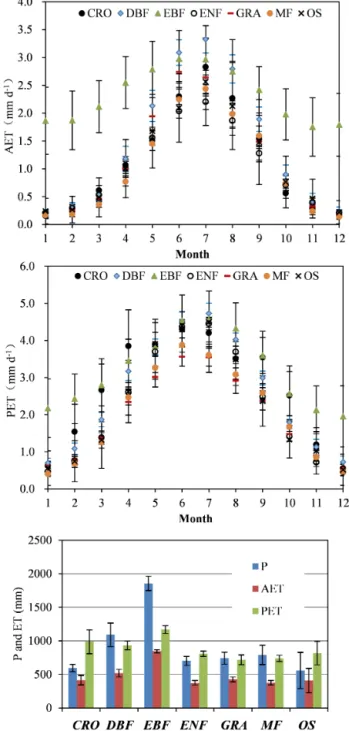
Figure 4.Monthly AET and PET, and annual total precipitation (P), AET, and PET for different vegetation types. The error bars are standard errors among different sites.
than other forest types (Fig. 2). Standard errors for grassland (GRA), evergreen needle leaf forest (ENF), and open shrub-land (OS) (0.10–0.17) were larger than for other shrub-land cover types (0.03–0.10) for April to August. EBF had higherKc
for all seasons than other land covers with a peak value of 0.91 (±0.08) in the winter season (Fig. 3). In winter seasons, cropland (CRO) and OS had the lowestKc: 0.25 (±0.006)
Figure 5.Variation of annualKcat different latitudes (lat):(a)cropland (CRO), deciduous broad leaf forest (DBF), and evergreen broad leaf forest (EBF);(b)evergreen needle leaf forest (ENF), grassland (GRA), mixed forest (MF), and open shrubland (OS). The absolute values of the latitude were used in EBF for sites in the Southern Hemisphere, and all the determination coefficients (R2)listed in the figure were significant (p< 0.05).
The mean annual Kc was 0.39 (±0.04), 0.47 (±0.05),
0.75 (±0.03), 0.45 (±0.02), 0.57 (±0.06), 0.45 (±0.05), and 0.40 (±0.04) for CRO, DBF, EBF, ENF, GRA, MF, and OS, respectively. Yearly average precipitation was higher in EBF and DBF than other land covers (Fig. 4). The precipitation ranking by land cover type was EBF > DBF > MF > GRA> ENF > CRO > OS. Consequently, OS, MF, GRA, CRO, and ENF had relatively lower yearly AET (376–425 mm) than EBF and DBF. Moreover, DBF, EBF, and CRO had higher PET than other vegetation sur-faces. The variations for monthly AET and PET were pre-sented in Fig. 4 to the contrasting patterns of these two vari-ables. The AET and PET reached maximum values 2.2–3.3 and 3.6–4.7 mm d−1in June or July (December or January
for the Southern Hemisphere), respectively.
3.2 Environmental controls onKc
As indicated in Eq. (1), factors such as temperature and so-lar radiation were used for PET calculations, and were not independent ofKc. Therefore, we chose other independent
factors to simulateKc. Site latitude is a readily available
vari-able for a particular location, but is crucial to the day length and incoming radiation over the year.
The results showed that annual Kc was negatively (p< 0.05) correlated with latitude (Fig. 5) for CRO, DBF, ENF, GRA, and MF with a determination coefficient (R2)
of 0.83, 0.59, 0.21, 0.72, and 0.52, respectively. For OS, an-nual mean Kc also decreased with the increase in site
lat-itude. Most of the study site fell between 30 and 60◦N in latitude.
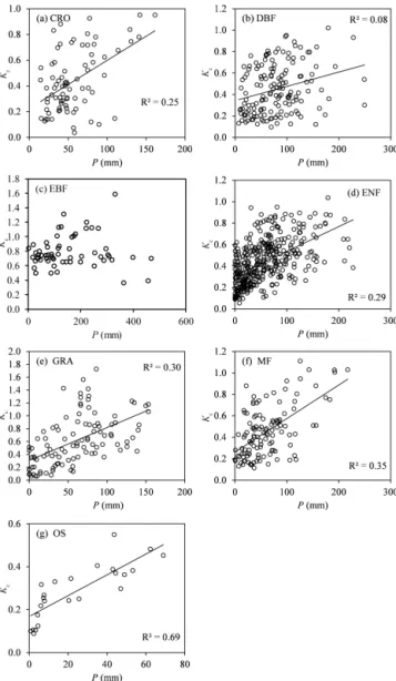
At the seasonal scale, the linear relationships be-tween monthly Kc and total monthly precipitation
dif-fered among different land cover types (Fig. 6). Monthly
Kc increased with monthly precipitation in the same
ecosystem type with the R2 ranking from high to low: OS > MF > GRA > ENF > CRO > DBF. The monthly Kc for
OS was especially sensitive to precipitation (R2=0.69,
p< 0.001). The monthlyKcfor EBF was not as sensitive to
precipitation as other ecosystems because EBF was generally found in a wet environment with a peak monthly precipita-tion of 468 mm. Moreover,Kcfor OS, GRA, and MF in
rel-atively drier environments had lower values (Fig. 2). There-fore,Kcwas closely related to the monthly precipitation.
In addition to growing season, site latitude, and monthly precipitation, leaf area index also affected the monthly Kc
(Fig. 7).Kc was obviously influenced by LAI for all land covers except EBF. The determination coefficients for differ-ent land covers were OS > MF=GRA > ENF > DBF > CRO. The LAI range was up to 6 m2m−2 in most land covers,
while it only reached 3–4 m2m−2in OS and CRO.
3.3 Kcmodels
A series of empiricalKc models have been developed
us-ing a multiple linear regression approach with precipitation, LAI, and site latitude as independent variables (Table 1). The monthly precipitation, LAI, and site latitude influence
Kc (p< 0.1) for most ecosystems studied in different
sea-sons except at EBF in summer and fall, and for OS in the spring. As annual precipitation increases, total leaf area in-creases; therefore,Kc increases for ENF in all seasons and most of the time for DBF and MF. As site latitude increases,
Kc values are found to decrease in some periods at CRO, DBF, and MF sites. In addition,Kcis closely correlated to
LAI, site latitude, and monthly precipitation at ENF in fall and OS in winter with anR2of 0.55 and 0.99, respectively. All land covers have peak values (0.53±0.04–1.01±0.17) in the summer months. Except for EBF and GRA,Kc
val-ues have a close relationship with the monthly precipitation in the summer withR2ranging from 0.21 to 0.90. The linear relationships are significant for most vegetation types, sug-gesting that the regression models (Table 1) can be used to estimate monthlyKcif LAI and precipitation for a specific
Table 1.Multiple linear regression relationships among crop coefficient and LAI, precipitation, and site latitude in different seasons.
IGBP Season N R2 Kc b a1 a2 a3
CRO Spring 24 0.16 0.31 0.242∗∗∗ 0.141∗
Summer 24 0.21 0.57 0.331∗∗ 0.0033∗
Fall 23 0.78 0.48 0.036 0.472∗∗∗
Winter 21 0.36 0.26 0.920∗∗∗ −0.0141∗∗
DBF Spring 39 0.49 0.30 0.479∗∗ −0.0076∗ 0.0022∗∗∗
Summer 39 0.42 0.65 0.536∗∗∗ 0.0011∗∗∗
Fall 39 0.13 0.60 0.462∗∗∗ 0.0014∗
Winter 39 0.15 0.30 0.713∗∗∗ −0.0094∗
EBF Spring 15 0.25 0.74 0.875∗∗∗ −0.0050∗
Summer 15 – 0.91 0.911∗∗∗
Fall 15 – 0.80 0.798∗∗∗
Winter 15 0.42 0.72 0.676∗∗∗ 0.050∗ −0.0050∗∗
ENF Spring 96 0.39 0.37 0.225∗∗∗ 0.060∗∗∗ 0.0017∗∗∗
Summer 99 0.59 0.49 0.211∗∗∗ 0.053∗∗∗ 0.0020∗∗∗
Fall 98 0.55 0.52 −0.040 0.066∗∗∗ 0.0049∗ 0.0025∗∗∗
Winter 92 0.21 0.44 0.293∗∗∗ 0.084∗ 0.0010∗
GRA Spring 27 0.48 0.45 0.237∗∗∗ 0.0052∗∗∗
Summer 27 0.23 0.86 0.572∗∗∗ 0.110∗ Fall 27 0.30 0.76 0.499∗∗∗ 0.123∗∗
Winter 27 0.26 0.41 0.256∗∗ 0.0038∗∗
MF Spring 30 0.67 0.31 0.099∗∗ 0.188∗∗∗ 0.0012∗∗∗
Summer 30 0.40 0.61 0.372∗∗∗ 0.0029∗∗∗
Fall 30 0.54 0.58 0.250∗∗∗ 0.071∗∗∗ 0.0018∗∗∗
Winter 30 0.13 0.33 0.961∗∗ −0.0136∗
OS Spring 6 – 0.23 0.230∗∗∗
Summer 6 0.90 0.35 −5.419∗ 0.1005∗ 0.0026∗
Fall 6 0.88 0.42 −9.921∗ 0.051∗ 0.1828∗
Winter 6 0.99 0.14 −4.919∗ 0.629∗ 0.0882∗ 0.0032∗
Note:Nis the number of observations used,R2the determination coefficient,K
cis the averageKcfor seasons.bis the
intercept of the multiple linear equation,a1the coefficient of LAI,a2the coefficient of site latitude (absolute values),a3
the coefficient of precipitation. IGBP is the International Geosphere-Biosphere Program land cover classification system: cropland (CRO), deciduous broad leaf forest (DBF), evergreen broad leaf forest (EBF), evergreen needle leaf forest (ENF), grassland (GRA), mixed forest (MF), and open shrubland (OS).∗∗∗,∗∗,∗stand forp< 0.001,p< 0.01,p< 0.1, and the blank spaces indicate nonsignificant values. In the Northern Hemisphere, spring is the months of February, March, and April; summer is May, June, and July; fall is August, September, and October; winter is November, December, and January. In the Southern Hemisphere, spring is August, September, and October; summer is November, December, and January; fall is February, March, and April; and winter is May, June, and July.
3.4 The validation of the regression models ofKc
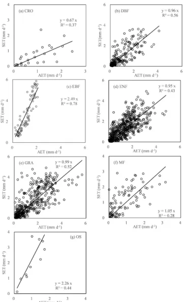
AllKcmultiple regression models for different seasons were validated by ecosystem type (Fig. 8). The model validation was carried out for 30 sites at a monthly scale. The results showed that the modeled AET calculated from the multiple
Kc models compared well to measurements withR2 rang-ing 0.28–0.56. Among the ecosystems, the model for DBF appeared to be the most accurate one, with anR2 of 0.56. However, model validation results for CRO, EBF, and OS were not as satisfactory as indicated by the slopes (< 1.0 or > 1.0) of the regression equations.
4 Discussion
Our study estimated annual and seasonal crop coefficient (Kc) for seven land cover types using measured global eddy
flux data. We comprehensively evaluated environmental con-trols (i.e., precipitation, LAI, and site latitude) on annual and growing seasonKcand developed a series of multiple linear regression models that can be used for estimating monthly AET over time and space for some vegetation types.
4.1 Crop coefficient variation in different seasons
Several recent studies had shown thatKc reached the
Figure 6. Relationships between the average monthly Kc and monthly precipitation (P, mm) for different vegetation surfaces. Panels(a–g)represent cropland (CRO), deciduous broad leaf for-est (DBF), evergreen broad leaf forfor-est (EBF), evergreen needle leaf forest (ENF), grassland (GRA), mixed forest (MF), and open shrub-land (OS), respectively. All the determination coefficients (R2) listed in the figure were significant (p< 0.001).
ecosystems, such as aP. euphraticaforest in the riparian area (Hou et al., 2010) in a desert environment, a watermelon crop covered with plastic mulch in Florida (Shukla et al., 2014a, b), soybean in Nebraska (Irmak et al., 2013b), and a temper-ate desert steppe in Inner Mongolia (Zhang et al., 2012). As Fig. 2 shows, most of the land covers have peak Kc during
June to August (in the Northern Hemisphere), while the sea-sonal patterns of ENF and EBF vary less than other surfaces. Vegetation growth for both the ENF and EBF sites is active throughout the year. The mean crop coefficient for medium-density fruit trees in the early growing season is about 0.5 (Allen et al., 1998; Allen and Pereira, 2009), which is
simi-Figure 7.Relationships between the average monthlyKcand leaf area index for different vegetation surfaces. Panels (a–g) stand for cropland (CRO), deciduous broad leaf forest (DBF), evergreen broad leaf forest (EBF), evergreen needle leaf forest (ENF), grass-land (GRA), mixed forest (MF), and open shrubgrass-land (OS). All the determination coefficients (R2)listed in the figure were significant (p< 0.05).
lar to those found for DBF or MF during April and May. In addition, the middle seasonKc values for apple and peach trees with active ground cover were higher thanKcfor DBF
sites during the summer. It is likely that the orchards had higher evapotranspiration rates than natural forests due to ir-rigation. We also find that the CRO has relatively low precip-itation with a high PET because of irrigation. The irrigation has been proven to be a determining factor for AET at the local and even at the global scale (Jaramillo and Destouni, 2015). Thus, the Kc for CRO mainly depends on the
Figure 8.Relationships between the simulated ET usingKcfrom Table 1 (SET) and the measured ET (AET) for different vegetation surfaces. Panels(a–f)stand for cropland (CRO), deciduous broad leaf forest (DBF), evergreen broad leaf forest (EBF), evergreen nee-dle leaf forest (ENF), grassland (GRA), mixed forest (MF), and open shrubland (OS). All the determination coefficients (R2)listed in the figure were significant (p< 0.001).
Kcin fall (Fig. 3). The soil water evaporation represents the
main water loss, which is thus a key component ofKcwhen the ecosystems lack leaves or plants in winter (Allen et al., 1998). Moreover, theKcis biologically meaningful in vege-tation type distribution (Stephenson, 1998); thus, when LAI becomes small for DBF during winter, the Kc reflects the characteristics of evaporation capacity for the ground sur-face.
4.2 Environmental control factors forKc
The ecosystem covers and the distributions of the vegetation classes are determined by the latitude (Potter et al., 1993). Crop coefficient varies predominately by ecosystems, and
Kc increases as the site latitude decreases for the same land
cover type (Fig. 5). As the latitude decreases, the increas-ing temperature and the solar radiation results of PET are increasing; thus, the acceleration for AET should be faster than PET. The reason may be that the vegetation character-istics are different for the same land cover type in different latitudes. Models developed from the FLUXNET data may be best used on flat areas for a specific latitude given that eddy covariance towers were generally installed on flat lands (Baldocchi et al., 2001). For areas with complex topography, the relationship betweenKc and site latitude may be more
complicated.
Spatial variations ofKcare characteristic of ecosystems,
butKc is also affected by climate factors such as rainfall.
For example,Kcwas highly correlated with precipitation for
most land covers (Fig. 6). The rainfall is the major source of soil water and AET in natural ecosystems (Parent and Anc-til, 2012). During dry years or periods, a lack of precipitation may cause a reduction of the leaf area index, andKcwill
de-crease. During rainy seasons, as leaf area index and stomatal conductance of trees and rain-fed crops increases, so does
Kc(Kar et al., 2006; Zeppel et al., 2008). Irrigation of crop-land is a primary mechanism for increasing yield (Fereres and Soriano, 2007; Du et al., 2015), so the CRO may have a high monthlyKceven at sites with a low precipitation. In contrast,Kc does not have a close relationship with
precip-itation under a wet environment. For example, the EBF site had a monthly precipitation as high as 468 mm month−1and
generally exceeded monthly AET. In an opposite case for the OS sites, monthly precipitation values were between 0.7 and 69 mm, andKcwas highly correlated with monthly
precipi-tation. Moreover, the time lag between precipitation and soil moisture might cause errors in calculating AET and model-ingKcin the long dry or wet season. However, at the monthly
scale, previous modeling work (Fang et al., 2015) suggests that considering a time lag does not increase the prediction power dramatically (G. Sun, personal communication, 2015). Besides precipitation, LAI also affectsKcin dry and semi-humid areas (Kang et al., 2003; Zhang et al., 2012). Unlike precipitation, LAI directly affectsKc in AET calculations (Tolk and Howell, 2001; Novák, 2012). InterannualKc
val-ues are stable at the GRA and OS sites due to the steady sea-sonal LAI between years while the plantation forest sites had a more dynamic LAI pattern (Marsal et al., 2014a). As the growth rate of the perennial plants could have large effects on the relationship betweenKcand LAI, long-term data are
needed to estimateKcas a function of all environmental
covers in different seasons (Table 1). Studies also show that monthly leaf stomatal resistance that varies over time is im-portant in estimating the seasonal crop coefficient for a cit-rus orchard (Taylor et al., 2015). The LAI and total monthly precipitation were considered as independent factors (Bond-Lamberty and Thomson, 2010) and both of them varied in both time and space while the site latitude only represented spatial influences onKc. The modeled AET was acceptable for DBF, ENF, GRA, and MF (Fig. 8), and could be used for monthly AET calculation for large-spatial-scale and homo-geneous ecosystems. The slope of CRO modeling ET to AET was 50 % below the 1 : 1 line which may be because the crops were irrigated when the soil lacked water content. Mean-while, the OS having a large proportion of bare soil with low soil water content may be the result of an overestimate in modeling ET. The lack of site samples may cause a low accuracy of validation in OS and EBF modeling ET. Thus, the multiple linear regression equations developed from this study take into account both spatial and temporal changes in land surface characteristics and offer a powerful tool for es-timating seasonal dynamics ofKcfor most ecosystems (Ta-ble 1).
5 Conclusions
In seeking a convenient method to calculate monthly AET at large spatial scales, we comprehensively examined the rela-tions betweenKcand environmental factors using eddy flux data from 81 sites (mainly in the Northern Hemisphere) with different land covers. We found thatKcvalues varied largely among CRO, DBF, EBF, GRA, and MF, and across seasons. Besides EBF, precipitation determined Kc in the growing seasons (such as summer) and was chosen as a key variable to calculateKc. We established multiple linear equations for
different land covers and seasons to model the dynamics of
Kc as function of LAI, site latitude, and monthly
precipita-tion. These empirical models could be helpful in calculating monthly AET at the regional scale with readily available cli-matic data and vegetation structure information. Our study extended the applications of the traditional Kc method for
estimating crop water use to estimating AET rates and evap-orative stress for natural ecosystems. Future studies should further test the applicability of the empiricalKcmodels
un-Acknowledgement. We are grateful for grants from the National Natural Science Foundation of China (no. 51309132), for sup-porting this collaborative work between Nanjing University of Information Science and Technology and the Eastern Forest Envi-ronmental Threat Assessment Center at the USDA Forest Service Southern Research Station. This work used eddy covariance data acquired by the FLUXNET community and in particular by the following networks: AmeriFlux (US Department of Energy, Bio-logical and Environmental Research, Terrestrial Carbon Program (DEFG02-04ER63917 and DE-FG02-04ER63911)), AfriFlux, AsiaFlux, CarboAfrica, CarboEuropeIP, CarboItaly, CarboMont, ChinaFlux, Fluxnet-Canada (supported by CFCAS, NSERC, BIOCAP, Environment Canada, and NRCan), GreenGrass, KoFlux, LBA, NECC, OzFlux, TCOS-Siberia, and the United States China Carbon Consortium (USCCC). We acknowledge the financial support to the eddy covariance data harmonization provided by CarboEuropeIP, FAO-GTOS-TCO, iLEAPS, Max Planck Institute for Biogeochemistry, National Science Foundation, University of Tuscia, Université Laval and Environment Canada, and the US Department of Energy, and the database development and technical support from Berkeley Water Center, Lawrence Berkeley National Laboratory, Microsoft Research eScience, Oak Ridge National Laboratory, University of California, Berkeley, and University of Virginia. This work also used MODIS land subset (Oak Ridge National Laboratory Distributed Active Archive Center (ORNL DAAC) 2011 MODIS subsetted land products, collection 5). We also thank the reviewers and associate editor for their constructive comments on the manuscript.
Edited by: K. Bishop
Reviewed by: three anonymous referees
References
Abrisqueta, I., Abrisqueta, J. M., Tapia, L. M., Munguía, J. P., Cone-jero, W., Vera, J., and Ruiz-Sánchez, M. C.: Basal crop coef-ficients for early-season peach trees, Agr. Water Manage., 121, 158–163, doi:10.1016/j.agwat.2013.02.001, 2013.
Alberto, M. C. R., Quilty, J. R., Buresh, R. J., Wassmann, R., Haidar, S., Correa, T. Q., and Sandro, J. M.: Actual evapotran-spiration and dual crop coefficients for dry-seeded rice and hy-brid maize grown with overhead sprinkler irrigation, Agr. Water Manage., 136, 1–12, doi:10.1016/j.agwat.2014.01.005, 2014. Allen, R. G. and Pereira, L. S.: Estimating crop coefficients from
Allen, R. G., Pereira, L. S., Raes, D., and Smith, M.: Crop evapo-transpiration, FAO irrigation and drainage paper, No. 56, 1998. Allen, R. G., Pruitt, W. O., Wright, J. L., Howell, T. A., Ventura,
F., Snyder, R., Itenfisu, D., Steduto, P., Berengena, J., Yrisarry, J. B., Smith, M., Pereira, L. S., Raes, D., Perrier, A., Alves, I., Walter, I., and Elliott, R.: A recommendation on standardized surface resistance for hourly calculation of reference ETo by the FAO56 Penman-Monteith method, Agr. Water Manage., 81, 1– 22, doi:10.1016/j.agwat.2005.03.007, 2006.
Allen, R. G., Pereira, L. S., Howell, T. A., and Jensen, M. E.: Evapotranspiration information reporting: I. Factors govern-ing measurement accuracy, Agr. Water Manage., 98, 899–920, doi:10.1016/j.agwat.2010.12.015, 2011.
Anda, A., Silva, J. A. T. D., and Soos, G.: Evapotranspira-tion and crop coefficient of common reed at the surround-ings of Lake Balaton, Hungary, Aquat. Botany, 116, 53–59, doi:10.1016/j.aquabot.2014.01.008, 2014.
Anderson, M. C., Allen, R. G., Morse, A., and Kustas, W. P.: Use of Landsat thermal imagery in monitoring evapotranspiration and managing water resources, Remote Sens. Environ., 122, 50–65, 2012.
Baldocchi, D., Falge, E., Gu, L., Olson, R., Hollinger, D., Run-ning, S., Anthoni, P., Bernhofer, C., Davis, K., and Evans, R.: FLUXNET: A new tool to study the temporal and spatial variabil-ity of ecosystem-scale carbon dioxide, water vapor, and energy flux densities, B. Am. Meteorol. Soc., 82, 2415–2434, 2001. Baldocchi, D. D. and Ryu, Y.: A synthesis of forest evaporation
fluxes – from days to years – as measured with eddy covariance, in: Forest Hydrology and Biogeochemistry, Springer, 101–116, 2011.
Bawazir, A. S., Luthy, R., King, J. P., Tanzy, B. F., and Solis, J.: Assessment of the crop coefficient for saltgrass under native ri-parian field conditions in the desert southwest, Hydrol. Process., 28, 6163–6171, doi:10.1002/Hyp.10100, 2014.
Bond-Lamberty, B. and Thomson, A.: Temperature-associated in-creases in the global soil respiration record, Nature, 464, 579– 582, 2010.
Budyko, M.: Climate and Life, Academic Press, New York, 1974. Consoli, S. and Vanella, D.: Mapping crop evapotranspiration by
in-tegrating vegetation indices into a soil water balance model, Agr. Water Manage., 143, 71–81, doi:10.1016/j.agwat.2014.06.012, 2014.
Descheemaeker, K., Raes, D., Allen, R., Nyssen, J., Poesen, J., Muys, B., Haile, M., and Deckers, J.: Two rapid appraisals of FAO-56 crop coefficients for semiarid natural vegetation of the northern Ethiopian highlands, J. Arid Environ., 75, 353–359, doi:10.1016/j.jaridenv.2010.12.002, 2011.
Ding, R. S., Tong, L., Li, F. S., Zhang, Y. Q., Hao, X. M., and Kang, S. Z.: Variations of crop coefficient and its influencing factors in an arid advective cropland of northwest China, Hydrol. Process., 29, 239–249, doi:10.1002/Hyp.10146, 2015.
Donohue, R. J., Roderick, M. L., and McVicar, T. R.: On the impor-tance of including vegetation dynamics in Budyko’s hydrological model, Hydrol. Earth Syst. Sci., 11, 983–995, doi:10.5194/hess-11-983-2007, 2007.
Du, T., Kang, S., Zhang, J., and Davies, W. J.: Deficit ir-rigation and sustainable water-resource strategies in agricul-ture for China’s food security, J. Exp. Bot., 66, 2253–2269, doi:10.1093/jxb/erv034, 2015.
Fang, Y., Sun, G., Caldwell, P., McNulty, S. G., Noormets, A., Domec, J. C., King, J., Zhang, Z., Zhang, X., and Lin, G.: Monthly land cover – evapotranspiration models derived from global eddy flux measurements and remote sensing data, Ecohy-drology, 9, 248–266, doi:10.1002/eco.1629, 2015.
Fereres, E. and Soriano, M. A.: Deficit irrigation for reducing agri-cultural water use, J. Exp. Bot., 58, 147–159, 2007.
Hao, L., Sun, G., Liu, Y., Gao, Z., He, J., Shi, T., and Wu, B.: Effects of precipitation on grassland ecosystem restoration under grazing exclusion in Inner Mongolia, China, Landscape Ecol., 29, 1657– 1673, doi:10.1007/s10980-014-0092-1, 2014.
Hao, L., Sun, G., Liu, Y., and Qian, H.: Integrated Modeling of Wa-ter Supply and Demand under Management Options and Climate Change Scenarios in Chifeng City, China, J. Am. Water Resour. As., 51, 655–671, 2015a.
Hao, L., Sun, G., Liu, Y., Wan, J., Qin, M., Qian, H., Liu, C., Zheng, J., John, R., Fan, P., and Chen, J.: Urbanization dra-matically altered the water balances of a paddy field-dominated basin in southern China, Hydrol. Earth Syst. Sci., 19, 3319–3331, doi:10.5194/hess-19-3319-2015, 2015b.
Hasper, T. B., Wallin, G., Lamba, S., Hall, M., Jaramillo, F., Laudon, H., Linder, S., Medhurst, J. L., Rantfors, M., Sig-urdsson, B. D., and Uddling, J.: Water use by Swedish bo-real forests in a changing climate, Funct. Ecol., 30, 690–699, doi:10.1111/1365-2435.12546, 2016.
Hou, L. G., Xiao, H. L., Si, J. H., Xiao, S. C., Zhou, M. X., and Yang, Y. G.: Evapotranspiration and crop coefficient of Populus euphratica Oliv forest during the growing season in the extreme arid region northwest China, Agr. Water Manage., 97, 351–356, 2010.
Irmak, S., Kabenge, I., Rudnick, D., Knezevic, S., Woodward, D., and Moravek, M.: Evapotranspiration crop coefficients for mixed riparian plant community and transpiration crop coeffi-cients for Common reed, Cottonwood and Peach-leaf willow in the Platte River Basin, Nebraska-USA, J. Hydrol., 481, 177–190, doi:10.1016/j.jhydrol.2012.12.032, 2013a.
Irmak, S., Odhiambo, L. O., Specht, J. E., and Djaman, K.: Hourly And Daily Single And Basal Evapotranspiration Crop Coeffi-cients as a Function Of Growing Degree Days, Days after Emer-gence, Leaf Area Index, Fractional Green Canopy Cover, And Plant Phenology for Soybean, T. ASABE, 56, 1785–1803, 2013b. Jaramillo, F., Prieto, C., Lyon, S. W., and Destouni, G.: Mul-timethod assessment of evapotranspiration shifts due to non-irrigated agricultural development in Sweden, J. Hydrol., 484, 55–62, doi:10.1016/j.jhydrol.2013.01.010, 2013.
Jaramillo, F. and Destouni, G.: Local flow regulation and irrigation raise global human water consumption and footprint, Science, 350, 1248–1251, doi:10.1126/science.aad1010, 2015.
Jung, M., Reichstein, M., Ciais, P., Seneviratne, S. I., Sheffield, J., Goulden, M. L., Bonan, G., Cescatti, A., Chen, J., and De Jeu, R.: Recent decline in the global land evapotranspiration trend due to limited moisture supply, Nature, 467, 951–954, 2010.
Kang, S., Gu, B., Du, T., and Zhang, J.: Crop coefficient and ratio of transpiration to evapotranspiration of winter wheat and maize in a semi-humid region, Agr. Water Manage., 59, 239–254, 2003. Kar, G., Verma, H. N., and Singh, R.: Effects of winter crop
sys-Marsal, J., Johnson, S., Casadesus, J., Lopez, G., Girona, J., and Stöckle, C.: Fraction of canopy intercepted radiation re-lates differently with crop coefficient depending on the season and the fruit tree species, Agr. Forest Meteorol., 184, 1–11, doi:10.1016/j.agrformet.2013.08.008, 2014b.
Mu, Q., Zhao, M., Kimball, J., McDowell, N., and Running, S.: A remotely sensed global terrestrial drought severity index, in: Evapotranspiration in the Soil-plant-atmosphere System, AGU Fall Meeting Abstracts, L02, 2012.
Novák, V.: Evapotranspiration in the Soil-plant-atmosphere System, Springer Science & Business Media, 2012.
Parent, A. C. and Anctil, F.: Quantifying evapotranspiration of a rainfed potato crop in South-eastern Canada using eddy covariance techniques, Agr. Water Manage., 113, 45–56, doi:10.1016/j.agwat.2012.06.014, 2012.
Pereira, L. S., Allen, R. G., Smith, M., and Raes, D.: Crop evapo-transpiration estimation with FAO56: Past and future, Agr. Water Manage., 147, 4–20, 2015.
Potter, C. S., Randerson, J. T., Field, C. B., Matson, P. A., Vitousek, P. M., Mooney, H. A., and Klooster, S. A.: Terrestrial ecosystem production: a process model based on global satellite and surface data, Global Biogeochem. Cy., 7, 811–841, 1993.
Rao, L., Sun, G., Ford, C., and Vose, J.: Modeling potential evap-otranspiration of two forested watersheds in the southern Ap-palachians, T. ASABE, 54, 2067–2078, 2011.
Shukla, S., Shrestha, N. K., and Goswami, D.: Evapotranspiration And Crop Coefficients for Seepage-Irrigated Watermelon with Plastic Mulch In a Sub-Tropical Region, T. ASABE, 57, 1017– 1028, 2014a.
Shukla, S., Shrestha, N. K., Jaber, F. H., Srivastava, S., Obreza, T. A., and Boman, B. J.: Evapotranspiration and crop coef-ficient for watermelon grown under plastic mulched condi-tions in sub-tropical Florida, Agr. Water Manage., 132, 1–9, doi:10.1016/j.agwat.2013.09.019, 2014b.
Stephenson, N.: Actual evapotranspiration and deficit: biologically meaningful correlates of vegetation distribution across spatial scales, J. Biogeogr., 25, 855–870, 1998.
Sun, G., Noormets, A., Gavazzi, M. J., McNulty, S. G., Chen, J., Domec, J. C., King, J. S., Amatya, D. M., and Sk-aggs, R. W.: Energy and water balance of two contrast-ing loblolly pine plantations on the lower coastal plain of North Carolina, USA, Forest Ecol. Manag., 259, 1299–1310, doi:10.1016/j.foreco.2009.09.016, 2010.
Sun, G., Alstad, K., Chen, J. Q., Chen, S. P., Ford, C. R., Lin, G. H., Liu, C. F., Lu, N., McNulty, S. G., Miao, H. X., Noormets, A., Vose, J. M., Wilske, B., Zeppel, M., Zhang, Y., and Zhang, Z. Q.: A general predictive model for estimating
Zhang, Y.: Drought impacts on ecosystem functions of the US National Forests and Grasslands: Part II assessment results and management implications, Forest Ecol. Manag., 353, 269–279, 2015a.
Sun, S., Sun, G., Caldwell, P., McNulty, S. G., Cohen, E., Xiao, J., and Zhang, Y.: Drought impacts on ecosystem functions of the US National Forests and Grasslands: Part I evaluation of a water and carbon balance model, Forest Ecol. Manag., 353, 260–268, 2015b.
Tabari, H., Grismer, M. E., and Trajkovic, S.: Comparative analysis of 31 reference evapotranspiration methods under humid condi-tions, Irrigation Sci., 31, 107–117, 2013.
Taylor, N., Mahohoma, W., Vahrmeijer, J., Gush, M., Allen, R. G., and Annandale, J. G.: Crop coefficient approaches based on fixed estimates of leaf resistance are not appropriate for estimating wa-ter use of citrus, Irrigation Sci., 33, 153–166, 2015.
Tolk, J. A. and Howell, T. A.: Measured and simulated evapotran-spiration of grain sorghum grown with full and limited irrigation in three high plains soils, T. ASAE, 44, 1553–1558, 2001. Vose, J. M., Sun, G., Ford, C. R., Bredemeier, M., Otsuki, K., Wei,
X., Zhang, Z., and Zhang, L.: Forest ecohydrological research in the 21st century: what are the critical needs?, Ecohydrology, 4, 146–158, 2011.
Wei, Z., Paredes, P., Liu, Y., Chi, W. W., and Pereira, L. S.: Mod-elling transpiration, soil evaporation and yield prediction of soy-bean in North China Plain, Agr. Water Manage., 147, 43–53, doi:10.1016/j.agwat.2014.05.004, 2015.
Xiao, J., Ollinger, S. V., Frolking, S., Hurtt, G. C., Hollinger, D. Y., Davis, K. J., Pan, Y., Zhang, X., Deng, F., and Chen, J.: Data-driven diagnostics of terrestrial carbon dynamics over North America, Agr. Forest Meteorol., 197, 142–157, 2014.
Zeppel, M. J. B., Macinnis-Ng, C. M. O., Yunusa, I. A. M., Whitley, R. J., and Earnus, D.: Long term trends of stand transpiration in a remnant forest during wet and dry years, J. Hydrol., 349, 200– 213, doi:10.1016/j.jhydrol.2007.11.001, 2008.
Zhang, B., Liu, Y., Xu, D., Zhao, N., Lei, B., Rosa, R. D., Paredes, P., Paço, T. A., and Pereira, L. S.: The dual crop coefficient ap-proach to estimate and partitioning evapotranspiration of the win-ter wheat–summer maize crop sequence in North China Plain, Irrigation Sci., 31, 1303–1316, 2013.
Zhang, F., Zhou, G. S., Wang, Y., Yang, F. L., and Nilsson, C.: Evap-otranspiration and crop coefficient for a temperate desert steppe ecosystem using eddy covariance in Inner Mongolia, China, Hy-drol. Process., 26, 379–386, 2012.
Zhang, Y., Song, C., Sun, G., Band, L. E., McNulty, S., Noormets, A., Zhang, Q., and Zhang, Z.: Development of a coupled carbon and water model for estimating global gross primary productivity and evapotranspiration based on eddy flux and remote sensing data, Agr. Forest Meteorol., 223, 116–131, 2016.