Two-Way Regionalized Classification of Multivariate Datasets and its Application to the Assessment of Hydrodynamic Dispersion

TWO-WAY REGIONALIZED CLASSIFICATION OF MULTIVARIATE DATA SETS AND ITS APPLICATION TO THE ASSESSMENT OF HYDRODYNAMIC DISPERSION1

by

Fernando António Leal Pacheco2,3 and Paulo Milton Barbosa Landim4

Corresponding Author: F.A.L. Pacheco

Geology Department, Trás-os-Montes and Alto Douro University, 5000 Vila Real, Portugal

Phone 351 259350280 fax 351 259350480 e-mail fpacheco@utad.pt 1 Received_______________; accepted_______________ 2

Geology Department, Trás-os-Montes and Alto Douro University, 5000 Vila Real, Portugal

3

Geophysical Center, Coimbra University, 3000 Coimbra, Portugal

4

Applied Geology Department, São Paulo State University, Rio Claro campus, 13506-900 Rio Claro(SP), Brazil.

Suggested Running Head: Application of two-way RC in the assessment of hydrodynamic dispersion

ABSTRACT

Zones of mixing between shallow groundwaters of different composition were unravelled by “two-way regionalized classification”, a technique based on Correspondence Analysis, Cluster Analysis and Discriminant Analysis, aided by gridding, map-overlay and contouring tools. The shallow groundwaters are from a granitoid plutonite in the Fundão region (central Portugal). Correspondence Analysis detected three natural clusters in the working data set: 1 – weathering; 2 - domestic effluents; 3 - fertilizers. Cluster Analysis set an alternative

distribution of the samples by the three clusters. Group memberships obtained by

Correspondence Analysis and by Cluster Analysis were optimized by Discriminant Analysis, gridded over the entire Fundão region, and converted into “two-way regionalized

classification” memberships as follows: codes 1, 2 or 3 were used when classification by Correspondence Analysis and Cluster Analysis produced the same results; code 0 when the grid node was first assigned to cluster 1 and then to cluster 2 or vice-versa (mixing between weathering and effluents); code 4 in the other cases (mixing between agriculture and the other influences). Code-3 areas were systematically surrounded by code-4 areas, an observation attributed to hydrodynamic dispersion. Accordingly, the extent of code-4 areas in two orthogonal directions was assumed proportional to the longitudinal and transverse dispersivities of local soils. The results (0.7-16.8 m and 0.4-4.3 m, respectively) are acceptable at the macroscopic scale. The ratios between longitudinal and transverse dispersivities (1.2-11.1) are also in agreement with results obtained by other studies.

KEY WORDS: Correspondence Analysis, Cluster Analysis, Discriminant Analysis, Surface Mapping Tools, Regionalized Classification, Hydrodynamic Dispersion

NOTATION

Below is the alphabetical list of mathematical symbols used throughout this paper.

Latin Symbols

d - geometric mean diameter of a granular material (e.g. soil sample)

D (DL, DT) - Coefficient of hydrodynamic dispersion (longitudinal and transverse)

Ei - classification score of group i

fi(x) - score of vector x in the frequency curve (f) of group i

F - factor

grad(h) - hydraulic gradient

h - number of rows along the height of a grid

k - number of groups present in a multivariate site-related data set K - hydraulic conductivity

l - number of columns along the width of a grid mt - total porosity

me - effective porosity

n - number of samples (or sites) in the working database

p - number of variables describing the samples (or sites) in the working database probi - prior probability of group’s i membership

Probi - posterior probability of group’s i membership S - matrix of within-group variances and covariances

t - time

v - velocity of a solute dissolved in water along the mean direction of flow

xp - vector containing the values of the p original (or X) variables x' - transpose of x

x

x

x

X - set of original variables in the working data set wij - loading of variable j in factor i

w%-Pollution - hydrochemical parameter discriminating between waters with

weathering-dominated chemistries and waters with chemistries controlled by anthropogenic inputs

w%-Agriculture - hydrochemical parameter discriminating between waters with

Greek Symbols

 (L, T) - mechanical dispersivity (longitudinal and transverse)

 - log standard deviation of a grain size distribution

 - identification code of a hybrid region

standard deviation of a membership probability distribution

INTRODUCTION

Regionalized Classification (RC) is defined as the probabilistic assignment of sites to groups by using Discriminant Analysis (DA). Following Olea (1999) and his predecessors Harff and Davis (1990), we see nothing conceptually new in RC but agree that some novelty is

introduced by this joint application of a number of well known mathematical, statistical and geostatistical techniques.

The start of RC requires a training set that usually is provided by Cluster Analysis (ClA). However, with conventional clustering algorithms the number of groups (k) is defined subjectively, either on the basis of external information or iteratively until a certain function is optimized. A second difficulty in applying RC is the assignment of sites to groups when probabilities are similar among clusters. Again, the problem is solved by assigning to group zero (i.e. by setting to hybrid) all sites for which the difference between the two highest probabilities are less than a pre-established (subjective) threshold.

The primary objective of this study is to clean RC from the reported drawbacks. To define k objectively we propose that it is selected by natural clustering. To identify the hybrid sites precisely, we propose that a RC based on the natural groupings (first-way RC) is

combined with another RC based on the ClA groupings (second-way RC). By looking simultaneously at two different perspectives of a same reality, we expect that the typical sites maintain their group memberships no matter which clustering method is used, whereas the atypical ones alternate among groups when the clustering technique is changed.

Consequently, the atypical sites are recast as hybrid sites and demarcated on a map as hybrid regions.

The spatial relation between true and hybrid regions of groundwater data sets may, in some cases, unravel the mixing between waters of different compositions. The distribution of membership probabilities within regions of fertilizer-dominated water chemistries resembles the distribution of solutes inside pulse-like contaminant plumes. Using the appropriate contaminant transport models, it is possible to quantify processes such as hydrodynamic

dispersion from solute distributions inside plumes. As a secondary objective we wished to assess hydrodynamic dispersion across the soils of our study area (Fundão region, central Portugal) using the membership distributions as analogs for solute distributions.

THE TWO-WAY RC APPROACH

The flowchart in Figure 1 summarizes the method of two-way RC. The sites of a multivariate database are initially assigned to k groups by natural clustering, and then the groups are interpreted in terms of controlling sources and/or processes. When working with groundwater databases, the selected method of natural clustering can be the RST algorithm used by Pacheco and Van der Weijden (1996), Pacheco (1998a) or Pacheco and others (1999), or can be the technique based on Correspondence Analysis (CA) that Pacheco (1998b)

developed. The first-way RC can pass through an optimization process using Discriminant Analysis (DA) or terminates. To start the second-way RC we run a conventional clustering algorithm like Ward’s method (1963) to obtain a sub-optimal non-natural distribution of the sites by the k groups that subsequently is optimized using DA. Node Analysis (NA) is a last step in two-way RC whereby the natural and non-natural group memberships are interpolated over grids of regularly spaced nodes. Nodes are then compared among grids, maintaining their original assignments or being reclassified as hybrid in a combined grid. Finally, constant membership contours are drawn across the study area that work as boundaries between different groups as well as between groups and hybrid regions.

The next sections outline the mathematical, statistical and geostatistical procedures involved in two-way RC. Detailed and more mechanically oriented descriptions of these methods are beyond the scope of this paper and can be found elsewhere (Kaufman and Rousseeuw, 1990; Jackson, 1991; Jobson, 1992; among many other neat textbooks). It also should be mentioned that we used Pacheco’s (1998b) approach to CA to define the natural clusters and Ward’s method to represent the technique of non-natural clustering.

Correspondence Analysis

In this study, CA is used as a natural clustering technique. As usual, the set of p original or X variables are first transformed onto a set of p factors or F variables in a manner that a major portion of the data variation is concentrated on just a few of the latter, the so-called k common factors. The relation between the F and X variables is set on the basis of a linear equation:

Fi = wi1X1 + wi2X2 + ... + wipXp. (1)

If the signs of factor loadings (wi coefficients) are equal, the corresponding X variables are

correlated positively in Fi, otherwise they are correlated negatively. From the observation of

these “sympathies” and “antipathies” among signs of factor loadings, Equation (1) may be rewritten in forms that encompass some physical or chemical meaning. That was the approach used by Pacheco (1998b). Working with a shallow groundwater database from a granitoid plutonite (Fundão, central Portugal), he separated waters with weathering-dominated chemistries from waters with compositions controlled by anthropogenic inputs, using the following hydrochemical parameter:

100

x

Pollution

Weathering

Pollution

Pollution

w%







 





 









Square brackets denote molar concentrations of chloride, sulphate, nitrate, bicarbonate and silica in a spring. Springs with w%-Pollution less than 50% have weathering-dominated water chemistries and springs with w%-Pollution greater than 50% have pollution-dominated water chemistries. The extent to which each component contributes to w%-Pollution is determined by the w1 values. Contaminated spring waters were further linked to sources such as farmland

100

x

e

Agricultur

Input

ents/Atm.

Dom. Efflu

e

Agricultur

e

Agricultur

w%











 

 

.







Cl

w

Input

ents/Atm.

Dom. Efflu

NO

w

SO

w

e

Agricultur

Springs with w%-Agriculture greater than 50% were assigned to agricultural activities and springs with w%-Agriculture less than 50% were attributed to urban pollution plus

atmospheric inputs.

In total, the hydrochemical parameters defined above accounted for about 80% of the system variance. The bi-univocal association (extent and significance) between

hydrochemical parameters and factors was checked by Multiple Linear Regression (MLR) with satisfactory results. Because the Fundão’s spring water chemistries have been explained by three different sources (weathering, agriculture and domestic effluents), Pacheco (1998b) classified his data set as a system of triple influence. In this study, these sources or influences provide a value for k, the number of natural clusters feeding Ward’s method of ClA.

Cluster Analysis (Ward’s Method)

ClA in this study is used as an alternative clustering technique. The adopted Ward’s method (1963) belongs to the category of agglomerative hierarchical methods. The aggregate is gradually built on a similarity coefficient between samples or sites. First the algorithm gathers all most-similar pairs and then aggregates the other samples/sites or already-formed groups according to their similarities until k groups are formed. Distinct from other

hierarchical methods, Ward’s method is a minimum variance agglomerative technique because the two clusters to be joined in each round of clustering are those generating the smallest increase in the within-cluster variation.

Discriminant Analysis

For the present case study, DA is used as a classification tool, namely for optimizing the location of sites pre-assigned by CA or ClA. A general approach to the problem of (re)classifying an observation x may be stated as follows:

)

ln(

prob

E









x

'



S



x



2

1

x

S

x'

where Ei is the classification score of group i; x' is the transpose of x;

x

x

of group i observations and the transpose of that vector, respectively; S-1 is the inverse of the within-group variance-covariance matrix; probi is the prior probability of group membership

manifest in the observed ni/n proportion, where ni is the number of observations in group i and

n the number of observations in the dataset. According to this criterion, an observation x will

be (re)classified into the group for which the E value is highest. The new (posterior) probability of group membership (Probi) is given by:

) ( ) ( 1 x x



where fi(x) is the score of x in the frequency curve of group i. The relation between prior and

post assignments is frequently reported in a confusion matrix that shows the number of correctly classified cases in the main diagonal and the number of misclassified cases in the off-diagonals. Confusion matrices are also useful to compare classification results obtained by different approaches [Eq. (2), Eq. (3), and Ward’s method].

Node Analysis

The scope of NA, as employed in this study, is threefold. First we looked at this procedure as a gridding tool. Using methods such as kriging, gridding produces a regularly

spaced array of z values from randomly spaced (x,y,z) observation points. When the (x,y,z) observations are spaced randomly over the study area, there are usually many holes in their distribution. Gridding fills in the holes by extrapolating or interpolating z values in those locations where no data exists. We interpolated the CA/DA group memberships to be used in NA over a grid with lh nodes, where l is the number of columns along the width and h the

number of rows along the height of the study area, and did the same with the ClA/DA results. After gridding we compared nodes between the CA/ClA or one-way RC grids and constructed a combined or two-way RC grid. If the membership of a node was equal in the first grids, then the node stayed in its group in the combined grid. Otherwise the node was reclassified as group- node (hybrid), where  is an arbitrary identification code. In the last stage of NA we drew constant membership contours across the grids that became boundaries between different groups and between groups and hybrid regions.

THE TWO-WAY RC MODEL FOR THE FUNDÃO AREA

In this study we used the set of 160 spring water samples that were collected in the Fundão area (central Portugal) by Van der Weijden and others (1983). The sampling was carried out in June-July. The samples’ locations are plotted in Figure 2 and the chemical analyses are given in the Appendix.

Results of CA/DA

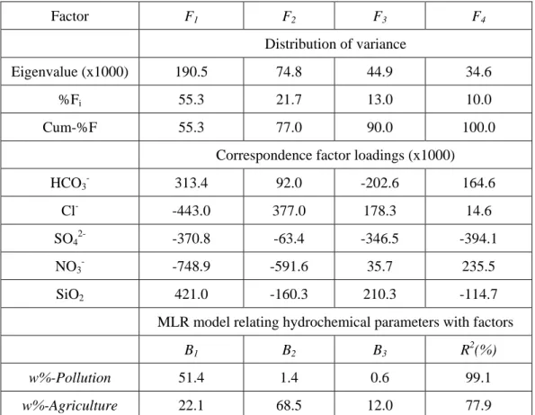
CA was applied by Pacheco (1998b) to the Fundão data set using the major anions and dissolved silica as variables (concentrations in mol/l). The results are shown in Table 1.

From the observation of sympathies and antipathies between factor loadings, the first two factors were represented by:

Pollution=443.0Cl-+370.8SO4 2-_ +748.9NO3 -_ Weathering=313.4HCO3 -_ +421.0SiO2 - the w%-Agriculture (factor two), with

Agriculture=63.4SO42-+591.6NO3-

Dom. Effluents/Atm. Input=377.0Cl-.

The water samples were assembled into three groups: 1 – weathering (w%-Pollution

< 50%); 2 - domestic effluents (w%-Pollution > 50% and w%-Agriculture < 50%); 3 -

farmland fertilizers (w%-Pollution > 50 % and w%-Agriculture > 50%). The results of this classification are listed in the Appendix under the heading CA/DA-Prior.

The relation between hydrochemical parameters and factors was set on the basis of MLR and the results are summarized in the last two rows of Table 1. The MLR model for

w%-Pollution holds a R2 = 99.1% indicating a tight regression between this parameter and F1,

but no similar link exists between the w%-Agriculture parameter and F2 (in the latter case R 2

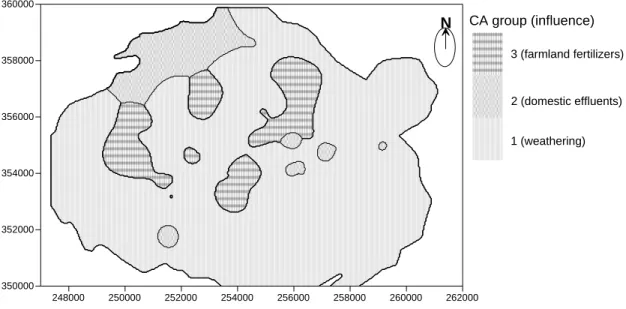
= 77.9%). In view of such uncertainty, we used DA to optimize the location of the samples with respect to the three pre-defined groups. The results are in column CA/DA-Post of the Appendix and reveal that 15 samples (9.4%) were reclassified into a different group. Using the optimized memberships of the samples and gridding as explained above, we drew Figure 3 that illustrates the areas of influence of each CA group.

Results of ClA/DA

The results from Ward’s method are described in detail in the Appendix (column ClA/DA-Prior). These groupings were used as a training set for DA which provided the post assignments listed in column ClA/DA-Post.

The confusion matrix comparing the CA/DA and ClA/DA results is shown in Table 2. There is little doubt that group A is equivalent to group 1 (the weathering group), but the associations between groups 2/3 and B/C are less evident. The medians of w%-Pollution and

w%-Agriculture suggest that group B and group 3 are influenced by farmland fertilizers,

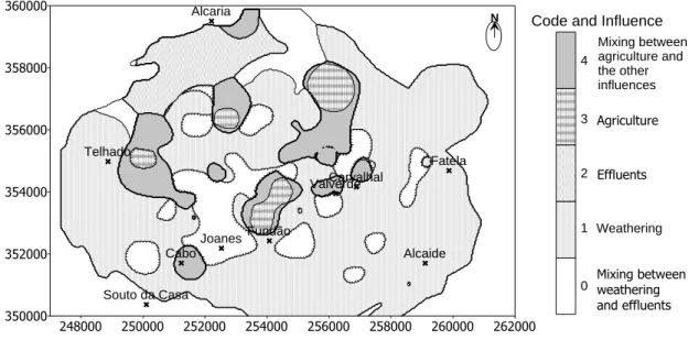
whereas group C, although falling in the field of weathering, has a median w%-Agriculture compatible with group 2 (influence by domestic effluents). Based on these associations we drew Figure 4 to show the areas of influence of each ClA/DA group.

Results of Node Analysis

Employing NA we combined Figures 3 and 4 obtaining Figure 5. The grids used were rectangles with l = 400 columns and h = 300 rows. The recasting of grid nodes was performed as follows: (1) when nodes in the one-way RC grids (Fig. 3 and 4) had the same value (1, 2 or 3 depending on whether their group memberships were 1/A, 2/C or 3/B) they preserved this value in the two-way RC (Fig. 5); (2) when group memberships in the original grids differ but one had the a value of 3 (fertilizer’s influence) they were recast as 4 (mixing between

fertilizer and other influences) in the combined grid; (3) in all other cases the two-way RC nodes were recast as 0 (mixing between weathering and domestic effluents).

The areas with weathering-dominated water chemistries occupy most of the studied region, working out as areas of background hydrochemistry. The dominance of effluents is restricted to the region of Alcaria, where the Meimoa river intersects the Zêzere river and some streamlets intersect the Meimoa river (Fig. 2). However, a substantial surface area upstream from the Meimoa river is occupied by regions where effluents blur the background compositions generated by weathering (white areas). Apparently the direct discharge of domestic effluents into streams and streamlets produces regions of mixing that are converted by some concentration process into a region of effluent-dominated water chemistries south of Alcaria. In all cases the areas with fertilizer-dominated water chemistries are spots surrounded by a zone of fluid mixing.

TWO-WAY RC AND THE ASSESSMENT OF HYDRODYNAMIC DISPERSION

Hydrodynamic dispersion of a solute in groundwater occurs as a consequence of two different processes: mechanical dispersion and molecular diffusion. Mechanical dispersion is a process of fluid mixing that causes a zone of mixing to develop between a fluid of one composition that is adjacent to or is being displaced by a fluid of another composition. It occurs as a result of variations around some mean velocity of flow. These variations are caused by the porous medium heterogeneities at the microscopic, macroscopic and megascopic scales (e.g. variations in the hydraulic conductivity, grain’s sorting, etc).

Molecular diffusion originates because of mixing caused by random molecular motions due to the thermal kinetic energy of the solute, i.e. it is a chemical rather than a physical (advective) process.

The results of two-way RC regarding the areas with fertilizer-dominated water chemistries (cross-hatched areas in Figure 5) suggest that some dispersion of the fertilizers took place after their application on farmland, because these areas are completely surrounded by a region of mixing (dark grey areas). It seems like the fertilizers applied in Spring (starting in early March) to feed the Summer crops have moved downstream and formed pulse-like contaminant plumes, which in turn have grown large and get diluted in their outer rims due to hydrodynamic dispersion. The sampling made in June-July worked out as a snapshot of the plumes when they were four months old. The purpose now is to quantify the hydrodynamic dispersion, but first some mathematical background must be introduced.

Mathematical Background on Hydrodynamic Dispersion

When a solute is subject to effective leaching, as usually happens in soils and saprolites derived from granites, mechanical dispersion grows several orders of magnitude higher than molecular diffusion, swamping the effects of this latter phenomenon (Pfannkuch, 1962). In such cases hydrodynamic dispersion is represented mathematically by:



m

h

grad

K

v





(

)

where D is the coefficient of hydrodynamic dispersion, v is the solute’s velocity in the mean direction of flow and  is a characteristic property of mechanical dispersivity; K, grad(h) and

me are the hydraulic conductivity, hydraulic gradient and effective porosity. Hydrodynamic

dispersion may be expressed by longitudinal (in the direction of flow) and transverse (at right angles) spreadings where the D and  coefficients are represented with L or T subscripts (e.g.

DL or T).

Assessment of the dispersion coefficients is essential for models of contaminant transport to work. Among the models in use, we focus on those dealing with localized and non-continuous sources of contamination, like the periodic application of fertilizers to farmland. According to these pulse-type models, the movement of a contaminant (e.g. sulphate) across the porous medium generates a growing plume due to hydrodynamic dispersion. One important feature of the concentration distribution inside the plume is that after a short period of time it becomes normal. The mean of the distribution describes the position of the plume and the variance (



2 T



t

D

t

D

2

2









The Analog Pulse-Type Model Based on Group Memberships

Application of pulse-type models [estimation of  in Equation (7)] requires that concentration distributions within contaminant plumes are well defined. This occurs when plumes are composed of a solute introduced artificially in the system (a tracer). In these cases solute concentrations inside and outside the plumes usually contrast. Contrarily, when plumes result from dissolution of fertilizers in ground waters also affected by weathering and

domestic effluents (present case), the overlapping of several and sometimes similar sources of solutes masks the boundaries between plumes and the natural environment, making it difficult to quantify the mass transport parameters. In these cases we would need first to define a sharp boundary around the plumes and then use a proxy to describe the concentration distributions inside them. We believe that this is performed adequately by the two-way RC approach: the boundary of a plume is defined by the outer limit of a dark grey area enclosing a cross-hatched area (Fig. 5). The concentrations are represented by the membership probabilities of groups linked to the agriculture influence (1/2(group 3+group B)), listed in the Appendix under the heading Prob-3/B.

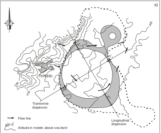
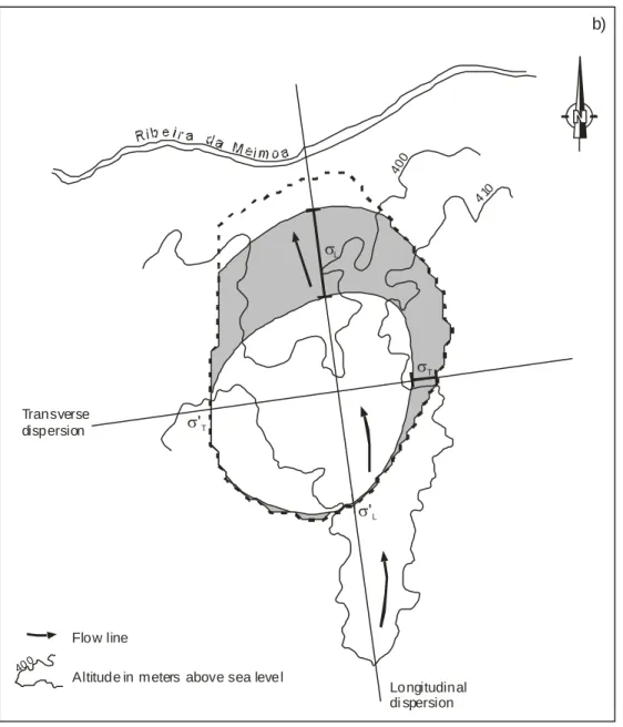
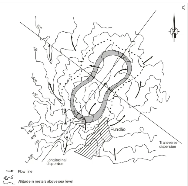
In total there are four contaminant plumes in Figure 5, which were termed Telhado, South of Alcaria, Fundão and North of Valverde in reference to the closest town. From data in column Prob-3/B of the Appendix, we drew contours of membership probability inside the plumes and shaded the space between those corresponding to the means and means minus standard deviations (Fig. 6a-d). The thicknesses of the shaded areas in the directions of elongation and at right angles are measures of L and , respectively.

Hydrology of the Fundão Soils

Apart from the estimation of , quantification of dispersivities [Eq. 6a] requires that some hydrologic information is available on the studied porous media, namely mean

velocities of flow, which in turn are dependent on hydraulic gradients, hydraulic

conductivities and effective porosities [Eq. 6b]. Hydraulic gradients may be approached by topographic gradients. The other necessary hydrologic information is compiled in the next paragraph.

Costa and others (1971) collected a set of 37 soil samples from the region of Fundão and analysed them for grain size (Table 3). Hydraulic conductivities were estimated from the grain size distributions using the formula of Krumbein and Monk (1943):

 31 . 1 2

760



d

e

K

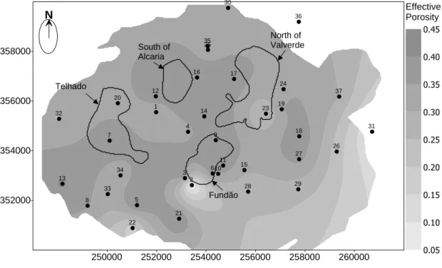
where K is the hydraulic conductivity given in darcys (conversion to m/s implies a division by 104000), d is the geometric mean diameter (in millimeters) and  the log standard deviation of the grain size distribution. The log(K) values are listed in the last column of Table 3 and their spatial distribution is shown in Figure 7. Effective porosities have been estimated by an analytical method cited in Custodio and Llamas (1983):

clay

loam

sand

-

m

m



















65

.

1

35

.

0

03

.

0

where mt and me are the total and effective porosities of the soil and  is its specific retention;

sand, loam and clay are the proportions of the sand, loam and clay fractions in the sample

(Table 3). For mt we assumed a value of 50%, which is common for soils derived from

granites. The me values obtained by Equation (9) were interpolated across the Fundão area

and some contours were drawn (Fig. 8).

Dispersivities of the Fundão Soils

From Figures 6a-d we estimated the plumes’





from Figures 6a-d, we determined flow velocities [Eq. 6b] that when combined with the previously calculated hydrodynamic dispersions gave estimates for the longitudinal and transverse dispersivities [Eq. 6a]. All results are shown in Table 4.

The values of L range from 0.7 to 16.8 m. They are acceptable because in this study

we are dealing with the assessment of dispersivities at the macroscopic scale. As expected, the

T values are always smaller than the L values. The ratios L/T are within the interval [1.2,

12.6] m, a range that has already been found by other authors. The use of a single t is

obviously a source of uncertainty because application of fertilizers is not restricted to a single day. The value of 4 months is the largest gap between the actions of fertilizing and water sampling. A value for the smallest gap would be 2 months or so, for crops seeded in late April. Adoption of t = 2 months would raise the L and T dispersivities by a factor of 2, but their ranges would be kept under acceptable values.

CONCLUSIONS

Hydrodynamic dispersion at the macroscopic and larger scales is an interesting and still unsolved research topic. In the previous sections of this paper we showed how the shapes and concentration distributions of contaminant plumes can be assessed by the application of our two-way RC and, notwithstanding limitations in accounting for the age of the plumes, demonstrated that quantification of mechanical dispersivities by this method leads to reliable results not only at the level of absolute values of the longitudinal and transverse components but also at the level of the ratios between them.

REFERENCES

Costa, C.V., Pereira, L.G., Portugal Ferreira, M. and Santos Oliveira, J.M., 1971, Distribuição de oligoelementes nas rochas e solos da região do Fundão: Memórias e Notícias (Publicações do Museu e Laboratório Mineralógico e Geológico da Universidade de Coimbra), v. 71, p. 1-37.

Custodio, E. and Llamas, M.R., 1983, Hidrología subterránea: Ediciones Omega, Barcelona, Spain, v. 1, 1157 p.

Domenico, P.A. and Schwartz, F.W., 1990, Physical and chemical hydrogeology: John Wiley & Sons, Inc., New York etc., 824 p.

Harff, J. and Davis, J.C., 1990, Regionalization in geology by multivariate classification: Mathematical Geology, v. 22, no. 5, p. 577-588.

Jackson, J. E., 1991, A user's guide to principal components: John Wiley & Sons Inc., New York etc., 569 p.

Jobson, J.D., 1992, Applied multivariate data analysis, v. 1 - Regression and experimental design: Springer-Verlag, New York, 621 p.

Kaufman, L. and Rousseeuw, P.J., 1990, Finding groups in data: John Wiley & Sons Inc., New York etc., 342 p.

Krumbein, W.C. and Monk, G.D., 1943, Permeability as a function of the size parameters of unconsolidated sand: Trans. Amer. Inst. Min. Met. Engrs., v. 151, p. 153-163.

Olea, R.A., 1999, Geostatistics for engineers and earth scientists: Kluwer Academic Publishers, chapter 14.

Pacheco, F.A.L., 1998a, Finding the number of natural clusters in groundwater data sets using the concept of equivalence class: Computers & Geosciences, v. 24, no. 1, p. 7-15.

Pacheco, F.A.L., 1998b, Application of correspondence analysis in the assessment of groundwater chemistry: Mathematical Geology, v. 30, no. 2, p. 129-161.

Pacheco, F.A.L and Van der Weijden, C. H., 1996, Contributions of water-rock interactions to the composition of groundwater in areas with sizeable anthropogenic input: a case study of the waters of the Fundão area, central Portugal: Water Resources Research, v. 32, no. 12, p. 3553-3570.

Pacheco, F.A.L., Sousa Oliveira, A., Van der Weijden, A.J. and Van der Weijden, C.H., 1999, Weathering, biomass production and groundwater chemistry in an area of dominant

anthropogenic influence, the Chaves-Vila pouca de Aguiar region, north of Portugal: Water, Air and Soil Pollution, v. 115, no. 1/4, p. 481-512.

Pfannkuch, H.O., 1962, Contribution à l'étude des deplacement des fluides miscible das un milieu poreux : Rev. Inst. Fr. Petrol., v. 18, no. 2, p. 215-270.

Van der Weijden, C.H., Oosterom, M.G., Bril, J., Walen, C.G., Vriend, S.P. and Zuurdeeg, B.W., 1983, Geochemical controls of transport and deposition of uranium from solution. Case study: Fundão, Portugal: Technical Report, Utrecht University, Institute of Earth Sciences, Department of Geochemistry, EC contract 007.79.3 EXU NL, 67p.

Ward, J.H., 1963, Hierarchical grouping to optimize an objective function: Journal of the American Statistical Association, v. 58, p. 238-244.

APPENDIX: Location of the sampling sites (Hayford-Gauss M and P coordinates). Concentrations of major anions and silica in the 160 spring water samples collected by Van der Weijden and others (1983); the values were scaled to mol/l. For some reason, some of the values in this appendix were transferred incorrectly from the original data set to Pacheco and Van der Weijden (1996) and Pacheco (1998b). Some values regarding the cations (not shown in this appendix) are also incorrect in those papers, and the correct values are (mol/l): K(215)=34, Mg(226)=65, Mg(269)=861, Ca(42)=107, Ca(85)=171, Ca(226)=131, Ca(267)=327, Ca(271)=128, and Ca(439)=157, where values within brackets represent sample numbers. The chart shows prior and post assignments of samples to the CA and ClA groups. Prob-3/B is the sample’s average posterior probability of group 3 (CA) and group B (ClA) memberships (agriculture influence).

Identification Raw data CA/DA ClA/DA Prob-3/B

nr M (m) P (m) [HCO3-] [Cl-] [SO42-] [NO3-] [SiO2] Prior Post Prior Post

28 253614 353895 780 440 356 371 656 3 1 C C 0.21 30 253789 353965 844 485 458 460 639 3 3 C C 0.33 31 253263 353298 490 423 185 387 506 3 3 A A 0.27 32 253228 353579 390 282 129 371 558 3 1 A A 0.24 35 252491 352105 729 347 341 221 614 1 1 C C 0.13 39 252631 354666 619 231 129 216 260 3 3 A A 0.23 41 251789 355052 261 189 198 55 463 1 1 A A 0.12 42 252526 355754 370 130 127 139 421 1 1 A A 0.16 45 254526 358596 1280 668 464 121 571 1 2 C C 0.03 51 253474 358982 780 499 458 189 100 2 2 C C 0.06 59 252281 358526 2260 2115 635 150 674 2 2 B C 0.02 60 253614 357403 560 248 158 63 524 1 1 A A 0.05 61 254105 357684 580 231 83 18 560 1 1 A A 0.02 63 253754 353298 229 790 735 998 399 3 3 B B 1.00 66 251579 353719 480 296 325 366 474 3 3 A A 0.37 67 251754 353509 1052 243 4 0 684 1 1 C C 0.00 71 250526 353263 639 183 433 0 626 1 1 C C 0.07 72 250421 352947 239 164 56 1 478 1 1 A A 0.05 74 249930 353123 660 149 44 32 609 1 1 A A 0.02 75 249719 352772 480 138 62 0 399 1 1 A A 0.05 76 249754 352421 810 155 92 0 503 1 1 C C 0.02 77 252035 352140 851 550 237 258 499 2 1 C C 0.11 78 251474 351930 918 1664 473 874 438 2 2 B B 0.61 79 250737 352035 410 181 125 121 634 1 1 A A 0.05 84 251649 353158 451 307 323 211 426 3 3 A A 0.27 85 251579 352982 590 169 94 82 606 1 1 A A 0.03 86 255017 353403 870 279 35 60 663 1 1 C C 0.01 87 256316 353158 451 243 177 1 613 1 1 A A 0.03 90 257438 355474 760 248 125 47 506 1 1 C A 0.03 92 258000 356737 580 186 117 0 552 1 1 A A 0.03 96 258386 355228 480 336 58 32 652 1 1 A A 0.01 99 259123 354982 600 567 366 37 353 2 2 C C 0.06 202 250175 355017 239 1297 1307 839 573 3 3 B B 0.91 203 250210 355579 610 372 417 185 440 2 3 C C 0.23

Identification Raw data CA/DA ClA/DA Prob-3/B nr M (m) P (m) [HCO3-] [Cl-] [SO42-] [NO3-] [SiO2] Prior Post Prior Post

204 251895 356807 352 254 172 158 657 1 1 A A 0.07 205 252561 357052 716 536 404 379 485 3 3 C C 0.30 206 251052 356281 472 677 289 37 441 2 1 C A 0.05 207 250421 354737 244 621 580 500 489 3 3 B C 0.50 208 250666 355298 328 181 171 92 474 1 1 A A 0.12 209 250456 353895 367 231 323 240 532 3 3 A A 0.28 210 250386 353368 388 183 76 82 626 1 1 A A 0.03 211 251789 356035 1080 395 383 71 587 1 1 C C 0.04 212 251930 355544 357 85 173 144 603 1 1 A A 0.10 213 252702 356351 429 691 431 855 405 3 3 B B 0.92 214 252351 354702 215 220 437 203 437 3 3 A A 0.38 215 252702 354877 690 121 173 18 564 1 1 C C 0.03 216 250245 352035 1113 189 227 53 660 1 1 C C 0.02 217 251298 352456 787 243 90 3 654 1 1 C C 0.01 218 252000 353754 2994 485 228 181 635 1 1 C C 0.00 219 250140 354561 167 762 139 871 465 3 3 B A 0.55 220 253403 359158 3655 2482 1047 1081 264 2 2 B B 0.50 221 254456 357438 477 209 137 3 522 1 1 A A 0.04 222 253544 357544 642 259 194 216 634 1 1 A A 0.08 223 253158 356947 326 254 371 435 485 3 3 A A 0.44 224 253509 356035 1155 130 138 77 411 1 1 C C 0.04 225 253263 355474 372 133 227 58 472 1 1 A A 0.13 226 253684 355579 436 113 158 85 545 1 1 A A 0.08 227 253965 355895 367 124 154 226 581 1 1 A A 0.15 228 252526 352245 836 268 342 177 750 1 1 C C 0.05 229 255684 351684 557 536 162 205 666 1 1 A A 0.04 230 257544 352456 664 203 318 21 546 1 1 C C 0.07 231 255193 352351 626 178 448 124 508 1 1 C C 0.22 232 254561 353333 334 175 81 435 745 3 1 A A 0.17 233 254456 353965 690 790 514 2903 687 3 3 B B 1.00 234 253579 354807 433 158 278 132 670 1 1 A A 0.09 235 255403 356947 523 155 70 65 668 1 1 A A 0.02 236 255649 357088 601 1354 1144 1387 586 3 3 B B 0.99 237 254877 356175 400 118 96 248 207 3 3 A A 0.35 238 255158 356386 438 141 135 68 535 1 1 A A 0.06 239 254772 355193 600 324 274 500 558 3 3 A A 0.38 241 260210 357193 231 79 24 61 514 1 1 A A 0.06 242 259754 357509 136 65 10 71 445 1 1 A A 0.09 243 254105 359333 1529 874 515 435 776 2 1 C C 0.07 244 255859 355824 323 265 336 250 476 3 3 A A 0.33 245 254912 354702 692 310 173 131 608 1 1 A C 0.04 246 254631 356351 564 127 151 131 519 1 1 A A 0.09

Identification Raw data CA/DA ClA/DA Prob-3/B nr M (m) P (m) [HCO3-] [Cl-] [SO42-] [NO3-] [SiO2] Prior Post Prior Post

247 254947 357193 454 282 372 166 532 3 1 A C 0.21 248 250596 355789 526 195 384 500 415 3 3 A C 0.47 249 248877 352947 408 107 170 52 560 1 1 A A 0.06 250 258561 357614 187 268 279 324 579 3 3 A A 0.32 251 258842 357368 203 93 15 35 467 1 1 A A 0.06 252 259088 356842 128 104 7 66 414 1 1 A A 0.10 253 259438 356175 249 90 66 61 619 1 1 A A 0.04 254 260000 355509 295 116 75 29 600 1 1 A A 0.03 255 260105 355509 293 124 72 66 672 1 1 A A 0.03 256 259614 356140 236 130 75 35 520 1 1 A A 0.06 257 259438 355930 243 144 99 140 613 1 1 A A 0.07 258 259193 356000 59 96 9 66 237 1 1 A A 0.21 259 258456 353824 723 262 173 190 740 1 1 A C 0.03 260 255403 353438 647 141 62 44 760 1 1 A A 0.01 261 256140 353965 675 931 365 452 620 2 1 C C 0.21 262 256035 354070 1047 3328 749 1516 617 2 2 B B 0.51 263 256105 354281 1721 3159 1450 1242 740 2 2 B B 0.50 264 255930 354737 451 333 204 250 550 3 1 A A 0.16 265 256000 354526 567 152 43 9 697 1 1 A A 0.01 266 256000 355052 533 1297 1784 532 486 2 2 B B 0.54 267 256456 354877 1278 564 113 182 739 1 1 C C 0.01 268 256526 355263 526 527 439 282 581 2 3 C C 0.25 269 256316 354105 877 6770 1117 1048 567 2 2 B B 0.50 270 257088 354702 1169 1326 675 726 452 2 2 B B 0.58 271 257754 354386 449 214 50 139 842 1 1 A A 0.01 272 257158 353789 367 259 12 187 573 1 1 A A 0.06 273 252877 351684 652 164 24 4 723 1 1 A A 0.01 274 255930 352631 470 305 105 150 530 1 1 A A 0.07 275 256316 352316 516 282 25 105 662 1 1 A A 0.02 276 256737 351895 531 480 71 176 615 1 1 A A 0.03 277 256877 352596 606 361 119 113 736 1 1 A A 0.02 278 257965 352210 375 203 37 113 760 1 1 A A 0.02 279 258526 352631 688 592 134 118 692 1 1 C A 0.01 280 259614 350912 434 152 23 13 583 1 1 A A 0.02 402 256631 350421 150 115 14 22 211 1 1 A A 0.16 404 256982 350526 308 188 19 32 399 1 1 A A 0.06 406 254281 359684 853 623 151 60 692 1 1 C C 0.01 407 254807 359474 2081 745 399 106 757 1 1 C C 0.00 408 257088 359052 551 268 140 113 711 1 1 A A 0.02 410 260666 354386 272 107 25 74 530 1 1 A A 0.05 411 261333 353579 214 199 93 30 209 1 1 A A 0.18 415 248631 355824 470 244 34 8 612 1 1 A A 0.01

Identification Raw data CA/DA ClA/DA Prob-3/B nr M (m) P (m) [HCO3-] [Cl-] [SO42-] [NO3-] [SiO2] Prior Post Prior Post

420 254702 350947 390 209 46 14 340 1 1 A A 0.07 421 255859 350842 353 188 45 23 339 1 1 A A 0.08 423 260421 354245 262 88 32 29 352 1 1 A A 0.10 424 258596 351298 365 232 79 81 445 1 1 A A 0.08 425 258596 351088 819 91 21 11 812 1 1 C C 0.00 427 259649 351333 433 162 10 30 534 1 1 A A 0.03 430 248702 357017 725 241 324 34 464 1 1 C C 0.09 432 260596 352807 338 161 19 25 689 1 1 A A 0.01 433 260386 352351 280 107 82 24 524 1 1 A A 0.05 434 260772 352456 292 79 16 13 524 1 1 A A 0.03 435 260456 351859 421 64 10 5 581 1 1 A A 0.02 438 256035 359298 430 152 60 30 487 1 1 A A 0.04 439 253719 351474 714 128 25 0 709 1 1 A A 0.01 440 254140 351228 636 127 58 7 729 1 1 A A 0.01 441 256702 351298 956 166 67 8 875 1 1 C C 0.00 442 258561 352175 607 832 50 75 838 1 1 C A 0.00 443 259649 354386 549 378 65 33 569 1 1 A A 0.02 444 259649 353333 351 157 27 36 442 1 1 A A 0.05 446 256526 354175 651 255 28 33 887 1 1 A A 0.00 447 256105 353438 974 533 189 107 548 1 1 C C 0.02 452 252631 352281 838 338 351 105 774 1 1 C C 0.03 453 251579 354386 1123 276 92 17 752 1 1 C C 0.00 457 250666 350631 566 93 3 1 568 1 1 A A 0.02 458 255509 351438 526 195 18 22 670 1 1 A A 0.01 463 248947 350386 231 241 67 31 366 1 1 A A 0.09 514 254737 356035 558 161 133 27 497 1 1 A A 0.05 522 253824 356281 1149 181 95 32 600 1 1 C C 0.01 523 252702 353579 650 302 299 34 860 1 1 C C 0.01 524 252842 354982 918 248 228 21 679 1 1 C C 0.01 525 251754 355649 503 126 138 48 554 1 1 A A 0.05 530 256140 353614 643 454 356 62 742 1 1 C C 0.03 534 257509 353123 310 277 162 100 604 1 1 A A 0.06 535 257754 352281 625 725 286 105 568 2 1 C C 0.04 536 255824 351719 529 236 111 42 431 1 1 A A 0.06 539 257509 354912 600 685 226 150 375 2 1 C A 0.08 540 256491 354105 520 224 46 63 806 1 1 A A 0.01 573 259298 355789 96 195 20 19 280 1 1 A A 0.13 574 258561 356105 652 914 189 29 515 2 1 C A 0.01 575 258842 355193 875 426 261 30 514 1 1 C C 0.03 583 248947 357895 305 2350 269 284 415 2 2 B A 0.19 589 256316 352316 501 205 39 24 679 1 1 A A 0.01 591 250421 357403 572 412 418 20 228 2 2 C C 0.08

TABLE LEGENDS

Table 1. Results of the CA procedure. Adapted from Pacheco (1998b). Symbols: %Fi - percentage of data variation explained by Fi; Cum-%F - cumulative %Fi; Bi - standardized

regression coefficient of factor Fi; R 2

- adjusted coefficient of multiple determination;

w%-Pollution and w%-Agriculture – hydrochemical parameters calculated by Equations (2) and

(3).

Table 2. Confusion matrix comparing the results obtained by CA/DA (1, 2 and 3) and ClA/DA (A, B and C) groupings. Associated medians of the Pollution and

w%-Agriculture parameters as determined by Equations (2) and (3).

Table 3. Grain size distributions, hydraulic conductivities and effective porosities of 37 soil samples from the Fundão region. Original data (grain sizes) compiled from Costa and others (1971). Hydraulic conductivities estimated by the method of Krumbein and Monk (1943), and effective porosities by a method cited in Custodio and Llamas (1983) assuming an average total porosity of 50%. Symbols: nr - number of the soil sample; M, P - Hayford-Gauss coordinates of the soil samples (locations in Figures 7 and 8); K - hydraulic conductivity; me - effective porosity.

Table 4. Results of the procedures used to estimate the longitudinal and transverse dispersivities of the Fundão soils. Symbols: me - effective porosity; K - hydraulic

conductivity; grad(h) - hydraulic gradient; v - mean velocity of flow; L, 'L, T, 'T -

standard deviations of group-3/B membership probabilities (spatial representation); DL, DT -

FIGURE CAPTIONS

Figure 1. Flowchart illustrating two-way regionalized classification of multivariate data sets.

Figure 2. Location of the Fundão area and water sampling sites. Adapted from Pacheco (1998b). Original drawings in Van der Weijden and others (1983).

Figure 3. Spatial distribution of group memberships determined by the results of CA optimized by DA.

Figure 4. Spatial distribution of group memberships determined by the results of ClA optimized by DA.

Figure 5. Results of node analysis.

Figure 6. Topography around the contaminant plumes: (a) Telhado, (b) South of Alcaria, (c) Fundão, and (d) North of Valverde. The plumes are represented by dashed thick polygons. The shaded areas describe the regions inside the plumes where group-3/B membership probabilities range from the mean to the mean minus standard deviation. The thickness of the shaded areas is a measure of Eq. (7)]. The samples’ group-3/B memberships are listed in the Appendix.

Figure 7. Spatial distribution of the Fundão soils' hydraulic conductivities. The numbers near the dots are sample numbers as listed in Table 3. The labelled polygons are the four

contaminant plumes.

Figure 8. Spatial distribution of the Fundão soils' effective porosities. The numbers near the dots are sample numbers as listed in Table 3. The labelled polygons are the four contaminant plumes.

TABLE 1 Factor F1 F2 F3 F4 Distribution of variance Eigenvalue (x1000) 190.5 74.8 44.9 34.6 %Fi 55.3 21.7 13.0 10.0 Cum-%F 55.3 77.0 90.0 100.0

Correspondence factor loadings (x1000)

HCO3- 313.4 92.0 -202.6 164.6 Cl- -443.0 377.0 178.3 14.6 SO4 2--370.8 -63.4 -346.5 -394.1 NO3 --748.9 -591.6 35.7 235.5 SiO2 421.0 -160.3 210.3 -114.7

MLR model relating hydrochemical parameters with factors

B1 B2 B3 R

2

(%)

w%-Pollution 51.4 1.4 0.6 99.1

TABLE 2

A B C Total w%-Pollution w%-Agriculture

1 88 0 36 124 29.0 35.6 2 1 7 5 13 74.2 36.1 3 12 5 6 23 63.3 64.4 Total 101 12 47 160 w%-Pollution 30.5 78.4 40.8 w%-Agriculture 37.5 56.7 38.7

TABLE 3

Identification Grain Size Distribution (ranges in mm, values in wt%) Physical Parameters

nr M (m) P (m) Sand Loam Clay LOG (K) me

>2 2-0.05 0.05-0.02 0.02-0.002 <0.002 1 251980 355554 24.6 51.0 6.2 10.4 5.7 -2.08 0.32 2 253424 352614 5.9 36.9 14.5 24.1 18.4 -2.52 0.05 3 253144 352897 11.4 63.9 6.3 9.6 3.4 -2.17 0.36 4 253271 354764 25.1 52.9 4.7 12.1 5.0 -2.06 0.33 5 251206 351810 18.5 67.1 5.7 6.4 1.5 -2.06 0.41 6 254266 353084 28.4 51.4 6.2 10.0 2.2 -2.03 0.38 7 250099 354408 18.2 65.3 3.8 8.0 3.2 -2.07 0.38 8 249208 351786 10.0 71.7 5.3 7.8 4.3 -2.14 0.36 9 254393 354426 9.2 72.1 4.9 11.4 1.5 -2.15 0.39 10 254490 353072 29.1 49.5 5.0 10.3 4.2 -2.04 0.35 11 254691 353406 8.9 71.7 5.0 11.2 1.3 -2.15 0.40 12 251966 356192 18.1 65.7 4.3 7.6 3.4 -2.07 0.38 13 248191 352669 12.5 77.8 1.8 5.2 2.5 -2.07 0.41 14 253926 355384 2.2 80.6 6.0 8.3 1.7 -2.19 0.40 15 255549 353221 3.0 65.2 10.0 15.0 4.8 -2.30 0.31 16 253636 356950 18.8 69.6 3.8 4.2 2.8 -2.04 0.40 17 255132 356889 18.5 66.8 3.5 7.4 3.2 -2.06 0.38 18 257768 354582 1.6 80.3 5.0 10.5 2.2 -2.20 0.38 19 257059 355671 2.3 81.0 1.3 9.8 5.3 -2.19 0.35 20 250432 355914 7.2 67.8 11.5 4.8 4.6 -2.21 0.34 21 252911 351265 3.2 82.2 4.7 7.8 1.1 -2.16 0.41 22 251028 350888 5.2 50.9 10.4 20.3 11.7 -2.39 0.18 23 256420 355492 3.0 65.9 7.1 12.1 10.2 -2.29 0.24 24 257132 356479 1.3 76.8 5.9 10.9 4.5 -2.23 0.34 25 254075 358061 5.2 74.8 2.4 10.3 6.8 -2.19 0.32 26 259283 353968 2.1 68.7 4.3 12.7 11.5 -2.28 0.23 27 257763 353661 21.4 63.4 3.0 6.8 4.4 -2.05 0.37 28 255701 352352 1.6 66.3 7.0 16.4 8.0 -2.31 0.26 29 257728 352449 3.5 65.1 7.4 13.2 7.6 -2.29 0.27 30 254891 359752 17.0 53.1 9.8 14.3 4.8 -2.17 0.31 31 260713 354768 10.8 30.2 9.8 29.9 14.9 -2.48 0.08 32 248056 355286 13.2 61.0 5.8 12.0 7.0 -2.17 0.30 33 250026 352255 3.9 73.7 3.8 11.5 6.1 -2.21 0.32 34 250539 353009 7.8 69.7 5.4 10.9 5.6 -2.18 0.33 35 254066 358209 6.0 71.7 6.6 10.6 4.4 -2.20 0.34 36 257749 359193 24.6 51.0 6.2 10.4 5.7 -2.08 0.32 37 259381 356181 4.9 68.0 7.1 12.6 6.4 -2.24 0.30

TABLE 4

Direction Parameter

Contaminant Plume

A B C D

Telhado South of Alcaria Fundão North of Valverde

Mean group-3/B probability 0.4 0.4 0.6 0.5

Associated standard deviation 0.1 0.2 0.1 0.1

me 0.35 0.38 0.35 0.33 LOG (K) -2.13 -2.08 -2.15 -2.18 grad(h) 0.041 0.0068 0.0382 0.0094 v x10-4 (m/s) 8.5 1.5 7.7 1.9 Longitudinal L (m) 328.75 445.47 117.85 276.54 'L (m) 200.18 13.21 92.8 202.47 DL (cm2/s) 33.7 25.4 5.3 27.7 L (m) 3.9 16.8 0.7 14.8 Transverse T (m) 129.16 124.3 98.76 237.58 'T (m) 29.46 5 94.84 20.74 DT (cm 2 /s) 3.0 2.0 4.5 8.0 T (m) 0.4 1.3 0.6 4.3 Cross DL/DT 11.1 12.6 1.2 3.4

FIGURE 1

Regionalized multivariate dataset

Sub-optimal non-natural clustering based on k Sub-optimal Natural clustering Confusion matrix Discriminant analysis Optimal clustering

Second-way regionalized classification First-way regionalized classification

Node analysis

Combined regionalized classification Number of groups

(k)

FIGURE 3 N 248000 250000 252000 254000 256000 258000 260000 262000 350000 352000 354000 356000 358000 360000 0 0.9 1.8 2.7 CA group (influence) 3 (farmland fertilizers) 2 (domestic effluents) 1 (weathering)

FIGURE 4 248000 250000 252000 254000 256000 258000 260000 262000 350000 352000 354000 356000 358000 360000 0 0.9 1.8 2.7 B (farmland fertilizers) C (domestic effluents) A (weathering) N

FIGURE 5 248000 250000 252000 254000 256000 258000 260000 262000 350000 352000 354000 356000 358000 360000 Fundão Souto da Casa Telhado Alcaria Alcaide Fatela ValverdeCarvalhal Joanes Cabo

Code and Influence

Agriculture Effluents Weathering Mixing between agriculture and the other influences Mixing between weathering and effluents N 4 3 2 1 0

FIGURE 6A Longitudinal dispersion Transverse dispersion 400 450 500 400

Al titude in meters above s ea level Flow line 'T L T 'L a)

FIGURE 6B Longitudinal di spersion Transverse dispersion 400 410 400 Flow line L 'L T 'T b)

FIGURE 6C Longitudinal dispersion Transverse dispersion 500 4 50 440 4 30 420 460 470 480 490 400 Flow line 'L L '_T T Fundão

Altitude in meters above sea level

FIGURE 6D Longitudi nal dispersion Transverse disper sion 400 45₀ 4 10 4 20 4 30 440 400 Flow line

Altitude in meters above sea level

'L L 'T T d) Ribe_{ira d} a M_eim oa Valverde Carvalhal

FIGURE 7 248000 250000 252000 254000 256000 258000 260000 262000 350000 352000 354000 356000 358000 360000 1 2 3 4 5 6 7 8 9 10 11 12 13 14 15 16 17 18 19 20 21 22 23 24 25 26 27 28 29 30 31 32 33 34 35 36 37 -3.00 -2.80 -2.60 -2.40 -2.20 -2.00 LOG (k) Telhado South of Alcaria Fundão North of Valverde

N

FIGURE 8 250000 252000 254000 256000 258000 260000 352000 354000 356000 358000 1 2 3 4 5 6 7 8 9 10 11 12 13 14 15 16 17 18 19 20 21 22 23 24 25 26 27 28 29 30 31 32 33 34 35 36 37 0.05 0.10 0.15 0.20 0.25 0.30 0.35 0.40 0.45 Effective Porosity N Telhado South of Alcaria Fundão North of Valverde