Spatial modelling of the temperature at the top of Permafrost in Cierva Point (Antarctic Peninsula)

(1)

Universidade de Lisboa

Instituto de Geografia e Ordenamento do Território

Spatial modelling of the Temperature at the Top of Permafrost in Cierva Point

(Antarctic Peninsula)

Sara Ramos Marín

Dissertação orientada pelo Prof. Dr. Gonçalo Brito Guapo Vieira e coorientada pelo

Dr. Gabriel Alejandro Goyanes

Mestrado em Sistemas de Informação Geográfica e Modelação Territorial

Aplicados ao Ordenamento

(2)

Universidade de Lisboa

Instituto de Geografia e Ordenamento do Território

Spatial modelling of the Temperature at the Top of Permafrost in Cierva Point

(Antarctic Peninsula)

Sara Ramos Marín

Dissertação orientada pelo Prof. Dr. Gonçalo Brito Guapo Vieira e coorientada pelo

Dr. Gabriel Alejandro Goyanes

Júri:

Presidente: Professor Doutor Eusébio Joaquim Marques dos Reis do Instituto de Geografia e Ordenamento do Território da Universidade de Lisboa.

Vogais:

- Professor Doutor Gonçalo Brito Guapo Teles Vieira do Instituto de Geografia e Ordenamento do Território da Universidade de Lisboa.

- Professor Doutor Marc Oliva i Franganillo do Departamento de Geografia da Universidad de Barcelona.

(3)

Acknowledgements

The completion of this master thesis has been much more than analysing data and writing an ordinary dissertation, it has been an opportunity to get involved in the world of permafrost research and polar science.

I would like to thank my supervisor, Professor Gonçalo Vieira, for trusting me for the development of this research and for giving me the chance to discover the beautiful area of Cierva Point to collect the data in-situ. Stepping in “the end of the world” and getting in contact with the Antarctic territory allowed me to better understand the importance of monitoring the impacts of climate change in such sensitive environment and empowered my motivation to carry out this study.

Many thanks to Gabriel Goyanes, who accompanied me on the journey and supported me in every adventure working on field. Without his patience, Antarctic experience and drone pilot skills, I would not have been able to get all the fundamental data indispensable to carry out this work.

Special acknowledgments to the Portuguese Polar Program 2017/18 (PROPOLAR) for funding this research and facilitating the logistics that make possible the larger scale project about “Permafrost and Climate Change in the Antarctic Peninsula” (PTDC/AAG-GLO/3908/2012 – FCT, Portugal). Also, to Ana Salomé for all the support provided during my trip to Antarctica and for her great skills to handle any kind of incident.

Thanks as well to the project “Impact of Recent Climate Warming on Active-Layer Dynamics, Permafrost, and Soil Properties on the Western Antarctic Peninsula” (ANT-6900673) from the National Science Foundation (USA), in which the boreholes used in this work were installed. On the framework of this project, Prof. James Bockheim and Dr. Kelly Wilhelm provided the shallow borehole data for the years from 2012 to 2014.

Always thankful with my father, Miguel Ramos, who introduced and guided me on my first steps into the world of polar sciences, with the passion and enthusiasm of who devoted his life to the research in Antarctica. Thanks as well to my mum, the one that stands my anxiety and always have the magic words to keep me calm in the most stressful situations.

Finally, yet important, thanks to all my colleagues, teachers and friends that helped me during the last two years, either with advice, knowledge or encouragement.

(4)

I

TABLE OF FIGURES

Figure 1. Distribution of permafrost in the North (left) and South (right) hemispheres (Brown et al., 1997)……... 2 Figure 2. Permafrost vertical structure defined by its ground thermal regime- trumpet curve (modified from:

Cassie, n.d.)………. 4

Figure 3. Helicopter shot from of the polygonal ground in the F6 camp on Lake Fryxell in Taylor Valley

(McMurdo, Dry Valleys region, Antarctica) (Ball, 2010)……….. 8

Figure 4. Tundra polygons and beaded drainage on the north slope in the Arctic National Wildlife Refuge, Alaska

(Shaw, 2015)………. 9

Figure 5. Circular thermokarst lakes in peatlands, Hudson Bay Lowlands, Manitoba. Natural Resources Canada

(de Schutter, 2004)……… 9

Figure 6. Open system pingo in upper Eskerdalen, 35 km east of Longyearbyen, Svalbard, Norway. (Christiansen,

n. d.)……….. 10

Figure 7. Polygonal patterned ground, Minna Bluff, Antarctica - South Pole (78 23' S, 166 19' E).

(Arthus-Bertrand, n. d.)……….. 11

Figure 8. Solifluction lobes on the Ulu Peninsula, James Ross Island, Antarctica (Bethan, 2017)……… 11 Figure 9. Rock and talus debris flowing downhill in a rock glacier near McCarthy, Alaska

(photo: Isabelle Gärtner-Roer) (Schaefer et al., 2012)……….14

Figure 10. Irregular settling due to permafrost thaw destroyed this apartment building in Cherski, Siberia

(photo: Vladimir Romanovsky) (Schaefer et al., 2012)……….. 15

Figure 11. Circumpolar Active Layer Monitoring (CALM) network and Thermal State of Permafrost (TSP) network

distribution (Schaefer, 2014)……… 17

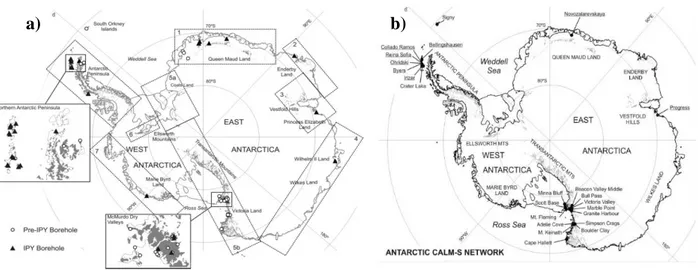
Figure 12. a) Antarctic permafrost monitoring boreholes (pre-and IPY installation) in relation to soil regions

according to Greene et al. (1997): 1. Queen Maud Land; 2. Enderby Land; 3. Vestford Hills; 4. Wilkes Land; 5a and b. Transantarctic Mountains; 6. Ellsworth Mountains; 7. Marie Byrd Land; 8.Antarctic Peninsula;b) Antarctic Circumpolar Active Layer Monitoring Network (CALM). New sites installed during the IPY are underlined (Vieira et al. 2010)……… 19

Figure 13. General permafrost distribution map in the Antarctic (modified from Bockheim, 1995)………. 21 Figure 14. a) Permafrost monitoring boreholes installed in the Antarctic Peninsula during the IPY

b) Active-layer thickness for selected boreholes. c) Mean ground surface and permafrost temperatures for selected boreholes (Vieira et al.,2010) ………. 24

Figure 15. Cierva Point ice-free peninsula, Hughes Bay (Danco Coast, Western Antarctic Peninsula) (Base Image

source: Google Earth, resolution: 2.4 m) ……… 26

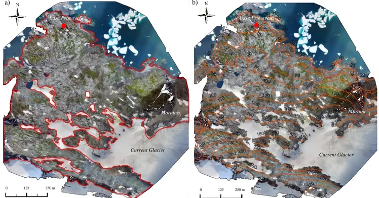
Figure 16. Cierva Point study area. a) Orthomosaic with indication of the ice-free terrains analysed in the

modelling (red line), b) Contour lines with altitude in meters (source: mosaic from UAV aerial imagery.

(7)

IV

Figure 17. Ground temperature boreholes distribution over Cierva Point. (Base image: Google Earth, resolution:

2.4m) ……… 31

Figure 18. a) iButton ground/air thermistors. b) Ground temperature GeoPrecision thermistor strings………….. 32 Figure 19. a) Mean daily ground temperatures measured in Site 1-Permafrost borehole from 2012 to 2018. b)

Differences in temperatures recorded after 18/Feb/17 thermistor replacement, from iButton to GeoPrecision. 33

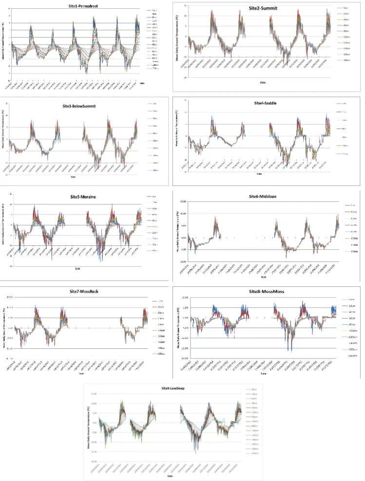
Figure 20. Mean daily ground temperatures in Cierva Point boreholes from 2012 to 2018. Note the different

data gaps……… 35

Figure 21. Air temperature miniloggers distributeon in Cierva Point. (Base image: Google Earth, resolution:

2.4m) ...……… 36

Figure 22. Mean daily air temperatures in the monitoring sites of Cierva Point ……… 37 Figure 23. Flight plans and photo shot locations of the UAV surveys conducted in Cierva Point with an overlap of

80% (Source: Pix4DMapper software processing) ……… 39

Figure 24. Example of images taken by the DJI-FC300S (RGB) in Cierva Point using the Phantom 3 UAV………… 39 Figure 25. a) Resulting photo mosaic of the area of study built up using UAV's aerial images . b) Digital Surface

Model of the study area derived from the orthomosaic. (Font: Pix4D software processing. Resolution: 6.51cm.41

Figure 26. a) Ortophotomosaic with level curves and clipped to the area of study. b) DSM clipped to the area of

study. Altitudes in both maps are expressed in meters above the ellipsoid WSG84 (Font: ArcMap 10.4

processing. Resolution: 6.51cm) ……….42

Figure 27. Ground temperature to depth plot of the maximum (red), mean (green) and minimum (blue) annual

ground temperatures constituting a borehole’s “trumpet profile” ………..……… 44

Figure 28. Influence of thermal conductivity on the ground thermal offset (modified from Williams & Smith,

1989) ………... 60

Figure 29. Moss-cover distribution in the modelled sectors of Cierva Point. White dotted region represents

areas of permanent snow, ponds or topographic errors standing out of the model. Spatial resolution: 1m ……. 61

Figure 30. Altitude distribution in the modelled sectors of Cierva Point, expressed in meters above the ellipsoid

WSG84. White dotted region represents areas of permanent snow, ponds or topographic errors standing out of the model. Spatial resolution: 1m ……… 62

Figure 31. Aspect distribution in the modelled sectors of Cierva Point. White dotted region represents areas of

permanent snow, ponds or topographic errors standing out of the model. Spatial resolution: 1m ………. 63

Figure 32. Distribution of the profile curvature in the modelled sectors of Cierva Point. White dotted region

represents areas of permanent snow, ponds or topographic errors standing out of the model. Spatial resolution: 1m ……….. 63

Figure 33. Distribution of the Type of substrate in the modelled sectors of Cierva Point. White dotted region

represents areas of permanent snow, ponds or topographic errors standing out of the model. Spatial resolution: 1m ……….. 65

Figure 34. Distribution of the Topographic Wetness Index in the modelled sectors of Cierva Point. White dotted

region represents areas of permanent snow, ponds or topographic errors standing out of the model. Spatial resolution: 1m ……….……….. 65

(8)

V

Figure 35. Air, ground surface and top of permafrost temperatures over the period from 2012 to 2018. Records

of air temperature from 2014 to 2016 were not available ………... 72

Figure 36. a) Observed ground temperature profile in Site 1 (Permafrost) between 2012 and 2018. Grey patches

represent gaps in the observed dataset. The red dotted line indicates the mean depth at the top of permafrost (5m) b) Trumpet profile built up using mean temperature values from 2012 to 2014. Black segments represent a 0.1°C thermistors’ measurement uncertainty……….. 73

Figure 37. a) Observed ground temperature profile in Site 2 (Summit) between 2012 and 2017. Grey patches

represent gaps in the observed dataset. b) Trumpet profile built up using mean temperature values from 2012 to 2014. Black segments represent a 0.5°C thermistors’ measurement uncertainty ……….. 75

Figure 38. a) Observed ground temperature profile in Site 3 (BelowSummit) between 2012 and 2017. Grey

patches represent gaps in the observed dataset. b) Trumpet profile built up using mean temperature values from 2012 to 2014. Black segments represent a 0.5°C thermistors’ measurement uncertainty ………. 75

Figure 39. a) Observed ground temperature profile in Site 4 (Saddle) between 2012 and 2017. Grey patches

represent gaps in the observed dataset. b) Trumpet profile built up using mean temperature values from 2012 to 2014. Black segments represent a 0.5°C thermistors’ measurement uncertainty ……….. 76 Figure 40. a) Observed ground temperature profile in Site 5 (Moraine) between 2012 and 2017. Grey patches represent gaps in the observed dataset. b) Trumpet profile built up using mean temperature values from 2012 to 2014. Black segments represent a 0.5°C thermistors’ measurement uncertainty. c) Trumpet profile after measurement uncertainty rectification down to 0.09°C ……….. 76

Figure 41. a) Observed ground temperature profile in Site 6 (MidSlope) between 2012 and 2017. Grey patches

represent gaps in the observed dataset. b) Trumpet profile built up using mean temperature values from 2012 to 2014. Black segments represent a 0.5°C thermistor’s measurement uncertainty ………77

Figure 42. a) Observed ground temperature profile in Site 7 (MossRock) between 2012 and 2017. Grey patches

Figure 43. a) Observed ground temperature profile in Site 8 (MossMoss) between 2012 and 2017. Grey patches

represent gaps in the observed dataset. b) Trumpet profile built up using mean temperature values from 2012 to 2014. Black segments represent a 0.5°C thermistors’ measurement uncertainty. c) Trumpet profile after measurement uncertainty rectification down to 0.04°C ……….. 78

Figure 44. a) Observed ground temperature profile in Site 9 (LowDeep) between 2012 and 2017. Grey patches

Figure 45. Local TTOP model validation by analysis of adjustment of TTOP model formula results to the

observed or estimated values determined first by graphical analysis of the trumpet profile ………... 83

Figure 46. a) Linear relationship between Ita and elevation. b) Linear relationship between Ifa and elevation.. 85 Figure 47. a) Normal Predicted Probability (P-P) plot for Ita as a dependent variable of elevation. b) Normal

(9)

VI

Figure 48. a) Plot of standardized residuals versus predicted values when performing a linear regression

between Ita and elevation. b) Plot of standardized residuals versus predicted values when performing a linear regression between Ita and elevation ……….. 86

Figure 49. a) Relationship between nt and moss cover. In the x-axis, a value of 0 stands for the absence of a

moss cover and a value of 1 for the presence. b) Linear relationship between nf and curvature ……….. 87

Figure 50. Normal Predicted Probability (P-P) plot for nf as a dependent variable of the terrain curvature ……. 88 Figure 51. Plot of standardized residuals versus predicted values when performing a linear regression between

nf and curvature ………... 89

Figure 52. a) Linear relationship between toffset and the Topographic Wetness Index (TWI) in bedrock areas.

b) Linear relationship between toffset and the Topographic Wetness Index (TWI) in unconsolidated soils or peat areas ……… 90

Figure 53. a) Normal Predicted Probability (P-P) plot for thermal offset as a dependent variable of the

Topographic Wetness Index (TWI) in bedrock areas. b) for thermal offset as a dependent variable of the

Topographic Wetness Index (TWI) in unconsolidated soils and peat areas ……… 91

Figure 54. a) Plot of standardized residuals versus predicted values when performing a linear regression

between thermal offset and TWI in bedrock areas. b) Plot of standardized residuals versus predicted values when performing a linear regression between thermal offset and TWI in unconsolidated soils and peat areas .91

Figure 55. Modelled air thawing index (It) distribution in Cierva Point based on data from the years 1 and 2.

White dotted region represents areas of permanent snow, ponds or topographic errors standing out of the model. Spatial resolution: 1m ………. 92

Figure 56. Modelled air freezing index (If) distribution in Cierva Point based on data from the years 1 and 2.

White dotted region represents areas of permanent snow, ponds or topographic errors standing out of the model. Spatial resolution: 1m ………. 93

Figure 57. Modelled thawing n-factor (nt) distribution in Cierva Point based on data from the years 1 and 2.

White dotted region include areas of permanent snow, ponds or topographic errors standing out of the model. Spatial resolution: 1m ……….. 93

Figure 58. Modelled thawing n-factor (nt) distribution in Cierva Point based on data from the years 1 and 2.

White dotted region include areas of permanent snow, ponds or topographic errors standing out of the model. Spatial resolution: 1m ………..94

Figure 59. Modelled thermal offset (toffset) distribution in Cierva Point based on data from the years 1 and 2.

White dotted region include areas of permanent snow, ponds or topographic errors standing out of the model. Spatial resolution: 1m ……….. 94

Figure 60. TTOP distribution over the area of study. Resulting TTOP values for each monitoring site are labelled.

Altitude lines are expressed in meters above the ellipsoid WGS84.White dotted region represents areas of permanent snow, ponds or topographic errors standing out of the model. Spatial resolution: 1m ………. 96

(10)

VII

Labels in bold at the right top of each site show the resulting TTOP after a 1°C increment on the MAAT. Label at the left top of each site show the modelled TTOP values in the current scenario. White dotted region represents areas of permanent snow, ponds or topographic errors standing out of the model. Spatial resolution: 1m ……. 99

Figure 62. a) Spatial distribution of TTOP classified separately in positive and negative TTOPs. b) Spatial

distribution of TTOP considering an increment of 1°C in the long-term MAAT. The map is classified in positive and negative TTOP. Spatial resolution: 1m ……… 102

Figure 63. Change in permafrost distribution in Cierva Point due to a long-term increase of 1 °C in the MAAT.

Green dots represent the 9 monitoring boreholes. White dotted region represents permanent snow, ponds or topographic errors standing out of the model. Spatial resolution: 1m ……….. 103

(11)

VIII

TABLE OF CHARTS

Table 1. Ground temperature monitoring boreholes in Cierva Point. Monitoring boreholes where presence of

permafrost was observed are highlighted in red colour. Elevation is expressed in meters above the ellipsoid WSG84 ……… 31

Table 2. Availability of air and ground temperature dataset over the full thawing and freezing cycles from 2012

to 2018. Years 1 and 2 are the only thawing and freezing cycles with a complete dataset for both air and ground temperatures (green checks, grey coloured). Years 3,4, and 6 have missing dataset values for either ground or air temperature during 30 or more days during the freezing/thawing cycle………. 38

Table 3. Summary of available data used for the analysis of the thermal regime and TTOP local and spatial

modelling ……….. 43

Table 4. Functions for the estimation of the minimum, mean and maximum annual ground temperature for

each boreholes’s trumpet profile. The adjustment of the estimation to the observed data is represented in the R2

column ………..……….……… 74

Table 5. Local ground thermal profile parameters derived from each borehole's trumpet profile. Green coloured

values were directly obtained from observed data. Orange values were estimated by extrapolation of observed data to the ZAA depth extent. results are shown with the uncertainty of the measurement ……….…. 79

Table 6. Air thawing and freezing indexes for years 1 and 2, and average values for both years. Values

expressed in °Cdays ……… 79

Table 7. Thawing and freezing ground surface indexes (at 5cm depth) for years 1 and 2, and average values for

both years. Values expressed in °Cdays ……….. 79

Table 8. Resulting nt and nf for computed using the average thawing and freezing air and surface indexes for

years 1 and 2 ………..…… 81

Table 9. Resulting values of seasonal thawing layer’s thermal offset computed using the average of year’s 1 and

2 ground temperature data ……….……… 81

Table 10. Results for all the TTOP model parameters (Is, Ia, n-factors, toffset), the depth at the Top of

Permafrost (TOP) and the Temperature at the Top Of Permafrost (TTOP) values estimated or observed using the analysis of the trumpet profile and TTOP results given by the TTOP model equation. All values are given

together with the propagated measurement uncertainty ………. 82

Table 11. Local values of terrain factors influencing on the different TTOP parameters in each monitoring

boreholes. In the Aspect row: N=North aspect, E=East aspect. In the Curvature row: possitive values represent concave profiles; negative values represent convex profiles ……….……….. 84

Table 12. Spearman correlation indexes between terrain factors and TTOP parameters ………..…………... 84 Table 13. Values for the locally observed and spatial estimated results of air indexes (Ita, Ifa), n-factors (nt,nf),

thermal offset (toffset) and TTOP model ………..…. 98

Table 14. Comparison between the mean measurement uncertainties and the error of the spatial estimation of

(12)

IX

TABLE OF EQUATIONS

Equation 1. a) TTOP model equation as a function of air freezing and thawing indexes, n-factors and the ratio of

thawed to frozen conductivities. b) TTOP parameters as a function of secondary parameters………... 48

Equation 2. a) TTOP model equation as a function of air freezing and thawing indexes, n-factors and the

seasonal thawing layer’s thermal offset (Way et al., 2016) ……… 48

Equation 3. TTOP as a function of mean annual ground temperature and the thermal offset ………... 49 Equation 4. Equations for the computation of freezing and thawing air indexes (Frauenfeld et al., 2007).50 Equation 5. Equations for the computation of freezing and thawing ground surface indexes ……… 51 Equation 6. Equations for the computation of freezing and thawing ground indexes at 5cm depth ……….. 52 Equation 7. Expressions for the computation of n-thawing (a) and n-freezing (b) factors (Smith & Riseborough,

1996) ……… 53

Equation 8. n-factors as expressed as the ratio between thawing and freezing indexes at 5cm depth and air

thawing and freezing indexes ………. 53

Equation 9. Thermal offset as a function of TTOP and MAGST (Burn & Smith, 1988) ……… 55 Equation 10. Active layer thermal offset related with its thermal regime and characteristics (Romanovsky &

Osterkamp,1995) ……… 56

Equation 11. Equation for the calculation of the Topographic Wetness Index (TWI) ………..64 Equation 12. Spearman Rank correlation formula (Statistical Solutions, 2018) ………. 66 Equation 13. a) Relationship function between Ita and elevation with respective estimation adjustment value of

R2_{. b) Relationship function between ……… 87}

Equation 14. a) Values assigned for nt in moss free and moss covered areas respectively. b) Relationship

function between nf and curvature with respective estimation adjustment value of R2_{.………..…… 89}

Equation 15. a) Relationship function between toffset and Topographic Wetness Index (TWI) with the respective

estimation adjustment value of R2_{. b) Relationship function between toffset and Topographic Wetness Index}

(13)

X

Abstract

The Western Antarctic Peninsula (WAP) has shown complex reactions to climate change in the last decades. To evaluate the changes occurring in these environments, permafrost and active layer monitoring and modelling are essential. In this dissertation, the characteristics of the ground temperature regime are analysed and the spatial distribution of the “Temperature at the Top of Permafrost” (TTOP) in Cierva Point (Danco Coast, WAP) is estimated using topo-climatic information over an area of 0.65 km2. With the results, the climate sensitivity of permafrost in this area and the potential impact of small climate change in its extent are evaluated.

A first evaluation of the temperature regimes allowed to determine the temperature and depth of the permafrost table and the ground thermal offset using observed borehole and climate data from nine different monitoring sites, in selected periods from 2012 to 2018. The top of permafrost was observed at depths of 0.4, 1 and 5m and the temperature at these depths was observed to be -1.4 ºC, -2.6 ºC and 1.2 ºC in these locations. For the monitoring boreholes where the top of permafrost was not reached, the depth of the top of permafrost was estimated to range between 0.4 and 5 m with temperatures ranging between -0.2 ºC and -2.6 ºC.

The results were used together with topographic data to implement the spatial TTOP model using a Geographical Information System (GIS)-based methodology to implement a high-resolution model (1 x 1 m grid cell) that allows a further insight into the spatial characteristics of permafrost.

Permafrost was estimated to be present in nearly 88% of the area and the lower TTOP values were found at high altitudes and unconsolidated soil or peat areas covered by moss. The highest TTOP results were found at low altitudes, bare surfaces and concave areas. Bare surfaces increase exposure to solar radiation during the summer and the concavity of the terrain promotes higher snowpack accumulation during the winter, which acts as a good thermal insulator hindering ground energy loses.

In the areas where the mean temperature at the top of permafrost was found to be higher than 0 ºC, permafrost is absent and the TTOP stands for the temperature at the base of the seasonal freezing layer.

(14)

XI

An increment of the TTOP was observed in case of a hypothetical long-term increase of 1 ºC in the MAAT and the results suggest the disappearance of nearly 50% of the current modelled permafrost area. Ground temperatures resulted to be more sensitive to the temperature increment at bare ground surfaces and/or concave sites. The less sensitive areas were the ones covered by moss formations as well as the most convex.

Permafrost degradation in Cierva Point, which is an Antarctic Specially Protected Area, may lead to significate impacts in the local ecosystem.

(15)

XII

Resumo

Durante as últimas décadas, a região ocidental da Península Antártica manifestou reações complexas às mudanças climáticas e as suas causas ainda não foram completamente compreendidas. Na segunda metade do século XX, foi observada uma tendência de aquecimento na Península Antártica. Contudo, a partir do início do século XXI, observou-se uma tendência para o arrefecimento em algumas regiões da Península. Com o objetivo de avaliar os efeitos destas reações nos ambientes livres de gelo da região, é importante a monitorização e modelação do permafrost e da camada ativa. O permafrost é definido como solo permanentemente congelado (mantém a temperatura a/ou abaixo de 0 ºC durante pelo menos dois anos). A camada compreendida entre a superfície do solo e o topo do permafrost, e que congela e descongela sazonalmente, é designada como “camada ativa”.

Nesta dissertação, são analisadas as caraterísticas do regime térmico do solo em Cierva Point (Costa de Danco Coast, Península Antártica Ocidental), numa área com 0.65 km2_e

apresenta-se um mapa da distribuição espacial da Temperatura no Topo do Permafrost (TTOP), usando dados topoclimáticos observados e modelizados. Com os resultados, é avaliada a sensibilidade climática do permafrost e o potencial impacte que mudanças na temperatura média anual poderão causar na sua extensão.

Inicialmente, foi desenvolvida uma análise do regime térmico do solo em nove locais com diferentes caraterísticas usando dados climáticos e de temperaturas do solo observados de 2012 a 2018 em perfurações instaladas na área de estudo. Esta análise, permitiu a determinação da espessura e da variabilidade interanual da camada ativa, da temperatura e profundidade do topo do permafrost, e finalmente, do offset térmico do solo (diferença de temperatura entre a superfície do solo e o topo do permafrost) nestes nove locais. O topo do

permafrost (TOP) foi encontrado em três dos nove locais com diferentes caraterísticas a 0,4, 1

e 5 m de profundidade e com temperaturas de -1.4 ºC, -2.6 ºC e 1.2 ºC, respetivamente. Contudo, os dados mostraram que a presença de permafrost é possível em oito dos nove locais, embora a profundidades maiores que aquelas de algumas perfurações, que apenas se encontram na camada ativa. As temperaturas no topo do permafrost estimadas nestes nove locais variam entre -0,2 ºC e -2,6 ºC. Em geral, o topo do permafrost foi observado a maior profundidade em locais com afloramentos rochosos, seguindo-se os depósitos não consolidados e os substratos orgânicos formados por musgos.

(16)

XIII

Os resultados da análise do regime térmico foram utilizados, em conjunto com dados topográficos, para a implementação de um modelo espacial da “Temperatura no Topo do

Permafrost” (TTOP) em toda a área de estudo, usando uma metodologia baseada nos

Sistemas de Informação Geográfica (SIG). Para a implementação do modelo TTOP, foram determinadas relações estatísticas entre os fatores topográficos e os parâmetros que constituem o modelo usando como base os dados observados nos nove locais. O software SPSS Statistics 25 foi o utilizado para estimar as correlações estatísticas entre fatores topográficos e parâmetros observados e para determinar as relações matemáticas existentes entre eles. Mais tarde, as relações estatísticas encontradas foram espacialmente computadas sob a área de estudo mediante o software ArcMap 10.4, e finalmente aplicou-se a equação do modelo sob a área de estudo completa.

O resultado foi um modelo TTOP de alta resolução (1 m) que oferece pela primeira vez uma perspectiva da distribuição espacial do permafrost em Cierva Point. Os resultados do modelo

TTOP ilustram os valores mais baixos (até -6.2 ºC) em solos orgânicos ou pouco consolidados

cobertos por musgos e em altitude, do que em áreas de menor altitude de rocha nua, húmidas e em terrenos côncavos

Os valores da Temperatura no Topo do Permafrost modelizada mais elevados (superiores a 0 ºC e até 3,5 ºC), encontraram-se em áreas mais baixas, húmidas e com topografia côncava. Nestas áreas, os valores resultantes representam, efetivamente, a temperatura na base do solo gelado sazonal.

Embora a profundidade do topo do permafrost seja desconhecida, os resultados mostram que o permafrost deverá estar presente em 88% da área de estudo, estando ausente especialmente em setores com solo nú em altitudes inferiores a 120 m e com topografia côncava.

O modelo espacial desenvolvido foi ainda usado para identificar a potencial sensibilidade do

permafrost face a um cenário hipotético de aumento da temperatura média anual do ar de

longo prazo de 1 ºC, considerando estáveis os restantes fatores como a precipitação, a neve, a humidade do solo, a distribuição dos musgos, etc. Os resultados indicam um significativo aumento na temperatura no topo do permafrost, correspondendo a um valor médio de +1.2 ºC, e o possível desaparecimento das condições para a manutenção do permafrost em cerca de 50% da área com permafrost na atualidade. A área com permafrost, ficaria então reduzida a cerca de 43% da área de estudo. Os setores mais sensíveis a esta mudança de temperatura são

(17)

XIV

as áreas localizadas a menor altitude, caraterizadas por superfícies nuas e/ou elevados valores de concavidade topográfica. As áreas menos sensíveis ao impacte do aumento de temperatura são as com cobertura de musgos, pois estes atuam como isolante térmico, assim como as áreas com topografia convexa.

A dinâmica do permafrost é especialmente importante em Cierva Point, que é uma Área Especialmente Protegida no quadro do Sistema do Tratado para a Antártida (ASPA), devido à presença de uma colónia de pinguins Gentoo, assim como de coberturas de líquenes e musgos. A redução da área com permafrost poderá influenciar significativamente o ecossistema local, pelos seus impactes na hidrologia e consequentemente, na flora. As propriedades impermeáveis do permafrost promovem o escoamento de água nos horizontes superficiais do solo ou à superfície, bem como a formação de pequenas lagoas temporárias. O descongelamento do permafrost, poderá induzir o aumento da infiltração em profundidade, reduzindo a água disponível para a vegetação.

(18)

XV

Acronyms

CALM: Circumpolar Active Layer Monitoring.

DSM: Digital Surface Model.

DZAA: Depth of Zero Annual Amplitude.

ECV: Essential Climate Variable.

GCOS: Global Climate Observing System.

GST: Ground Surface Temperature.

GTN-P: Global Terrestrial Network for Permafrost.

IPA: International Permafrost Association.

IPCC: Intergovernmental Panel on Climate Change.

MAGST: Mean Annual Ground Surface Temperature.

MaxAST: Maximum Annual Surface Temperature.

MDAT: Mean Daily Air Temperature.

MinAST: Minimum Annual Surface Temperature.

Toffset: Thermal offset.

TSP: Thermal State of Permafrost.

TTOP: Temperature at the Top Of Permafrost.

TWI: Topographic Wetness Index.

UNEP: United Nations Environmental Programme.

UNFCC: United Nations Framework Convention on Climate Change.

WAP: Western Antarctic Peninsula.

WMO: World Meteorological Organization.

(19)

1

1 Introduction

1.1 Objectives

The main objective of this dissertation is to characterize the permafrost in Cierva Point (Western Antarctic Peninsula) and evaluate its climate sensitivity by assessing the main potential impact of small climate changes in the permafrost extent of this ice-free environment area. In order to achieve this goal, we analysed the area’s ground temperature regime and created a GIS-based spatial model of the Temperature at the Top Of Permafrost (TTOP) based on statistical relations between certain topographic factors and locally computed TTOP parameters from climate observed data.

This work is included on the larger-scale framework of permafrost research in the ice-free terrestrial environments of Western Antarctic Peninsula, which aim to evaluate permafrost dynamics and its linkages to recent climate changes through systematic and long-term monitoring and modelling of ground and climate properties. The project is conducted by the CEG/IGOT team of the University of Lisbon, within the ANTPAS/SCAR expert group.

1.2 An overview of Permafrost and its global significance

1.2.1 WHAT IS PERMAFROST?

Permafrost is ground at or below the freezing point of water (0°C, 32°F) for at least two consecutive years (Brown et al., 1998). Permafrost forms in cold climates generally distinct by long winters without much of snow and short, dry and cold summers. In regions with such this climate, some of the ground frozen during the winter will not completely thaw during the summer; therefore, a permanent frozen layer will form and continue to grow downward gradually each year constituting the permafrost (Péwé, 1979).

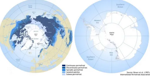
Permafrost is distributed on Earth covering great stretches of land at high latitudes and altitudes in both hemispheres. In the Northern Hemisphere, permafrost occupies about 24% of the exposed land area in the Arctic and sub-Arctic, including large areas in Russia, Alaska and Canada. In the Southern Hemisphere, permafrost occurs in most ice-free regions of Antarctica (Schaefer et al., 2012; Bockheim et al., 2012). Alpine permafrost may exist at high altitudes in much lower latitudes, being present in the high mountains of South America, Central Asia, the United States and Europe (Péwé, 1979).

(20)

2 1.2.2 DISTRIBUTION OF PERMAFROST

Permafrost regions are classified into zones based on its spatial distribution. “Continuous

permafrost” zones have permafrost underlying 90-100% of the land area; “discontinuous permafrost” zones have 50-90% of permafrost; and “sporadic permafrost” around the

10-50%. “Isolated patches” refer to regions where permafrost underlies less than 10% of the land area (Schaefer et al., 2012). Permafrost also occurs subsea on the continental shelves of the surrounding continent of the Arctic Ocean and Antarctica.

In the Northern Hemisphere permafrost occurs almost continuously in large areas, being normally absent under lakes and rivers that do not freeze to the bottom (Péwé, 1979). The location of the boundary of the continuous permafrost zone variates around the world because of regional climate controls. In areas characterized by warmer climates, permafrost occurs only in sheltered locations, usually with a north aspect (in the Northern Hemisphere) or south aspect (in the South Hemisphere), creating discontinuous, sporadic or isolated permafrost.

In the Southern Hemisphere, most of the Antarctic continent is overlain by glaciers and liable to basal melting (Zoltikov, 1962). The exposed ice-free land of Antarctica is extensively underlain with permafrost, some of which is liable to warming and thawing along the coastline (Campbell & Claridge, 2009).

Figure 1 represents the distribution of different types of permafrost in both South and North hemispheres.

(21)

3

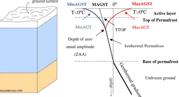
1.2.2 PERMAFROST STRUCTURE AND THERMAL REGIME

The vertical structure of permafrost is determined by the ground temperatures at different depths and is represented in Figure 2.

When permafrost is present in areas not overlain by ice, it occurs beneath a layer of soil, rock or sediment, which freezes and thaws annually, which is called the active layer (Staff, 2014). The active layer generally starts thawing in spring after snow melt and may stay thawed until autumn, while its maximum depth is reached in late summer. It begins to refreeze in autumn with the onset of winter and is completely frozen by late winter or early spring (Schaefer et al., 2012).

The active layer thickness is the annual maximum thaw depth at the end of the summer. It depends mainly on the moisture content, being thinner in wet, organic sediments and thicker in well-drained gravels or bedrock. Active layer thickness can be less than 30 cm in continuous permafrost along the Arctic coast and the Antarctic continent, where values range generally from 0.2 to 0.7 m, occasionally with >0.9 m in coastal sites and with very shallow active layers (<0.1 m) at high elevation sites (Vieira et al., 2010). The active layer thickness usually reaches 2 m or more in discontinuous permafrost of Southern Siberia, and several meters in the European Alps and on the Qinghai-Tibetan Plateau (Schaefer et al., 2012). In the Antarctic Peninsula, the active layer thickness was found to be greater than 0.9 m on monitored sites at unconsolidated materials in the South Shetlands Islands, and around 0.3 m in Deception Island (Vieira et al., 2010).

Under the active layer, permafrost occurs at the depth where the maximum annual temperature remains below 0 ºC, and is bounded on the top by the Top of Permafrost (TOP) and on the bottom by the Base of Permafrost (BOF) (Schaefer et al., 2012).

(22)

4

The annual variations of air temperature from winter to summer is revealed in the active layer and in the few first meters of the permafrost. In this layer, the ground temperature profile over a temperature to depth graph (Figure 2), presents three different curves that represent the variation of ground temperature with depth. The red curve represents the Maximum Annual

Ground Temperature (MaxAGT), the dotted line represents the Mean Annual Ground Temperature (MAGT) and the Minimum Annual Ground Temperature is represented by the

blue curve (MinAGT).

The MaxAGT decreases with depth being the depth at which the maximum annual temperature reaches 0º C considered the base of the active layer, and the top of permafrost, which is known as Temperature at the Top Of Permafrost (TTOP). The point where the red curve crosses the ground surface represents the Maximum Annual Ground Surface

Temperature (MaxAGST).

The MinAGT increases with depth being and the point where the blue curve crosses the ground surface represent the Minimum Annual Ground Surface Temperature (MinAGST). The MAGT can either increase or decrease depending on a positive or negative ground

thermal offset. The thermal offset’s magnitude is the difference between the mean annual

ground temperature at the top of permafrost and the MAGST, and it depends on the soil thermal properties. MAGST 0º MaxAGST MinAGST T<0ºC T>0ºC Isothermal Permafrost Unfrozen ground Base of permafrost MinAGT Depth of zero anual amplitude (ZAA) Active layer Top of Permafrost MaxAGT TTOP

Figure 2. Permafrost vertical structure defined by its ground thermal regime- trumpet curve (modified from:

(23)

5

The point where the dotted line crosses the surface represents the Mean Annual Ground

Surface Temperature (MAGST).

Despite the curve of the MAGT being often considered linear for simplification of the modelling, Goodrich (1978) showed that the MAGT warming at depth is not linear, but offsets to progressively lower values at depth within the active layer (Smith & Riseborough, 1996).

Under the surface, the seasonal ground temperature signal becomes smaller with depth due to the thermal balance between the heat flow from the Earth’s interior and that flowing outward into the atmosphere. When the amount of geothermal heat reaching the permafrost equals the heat lost to the atmosphere, the permafrost temperature reaches equilibrium and becomes seasonally stable at the depth of Zero Annual Amplitude (ZAA) (Péwé, 1979). The temperature at the Z depth is known as the Temperature at the depth of Zero Annual

Amplitude (TZAA). Because the maximum temperature at the top of permafrost is 0 ºC, no

significant phase change occurs at lower depths, such that soil thermal properties below the active layer remain relatively constant. For practical purposes, the temperature at the top of permafrost should be close to the temperature measured at the depth of zero annual amplitude (Smith & Riseborough, 1996).

Below the ZAA depth, the temperature of permafrost does not change seasonally, and hence this layer is named isothermal permafrost (Delisle, 2007). In the isothermal permafrost layer, the temperature increases steadily under the influence of heat from the Earth’s interior until overpassing 0 ºC due to the geothermal gradient. This point constitutes the base of permafrost

(BOP) (Péwé, 1979).

1.2.3 CONTROLLING FACTORS IN PERMAFROST: CLIMATE, WATER BODIES, SOLAR RADIATION, VEGETATION AND SNOW

The distribution and thickness of permafrost are directly affected by climate, ground properties and geothermal gradient, topography, snow, vegetation and water cover (Péwé, 2016).

(24)

6 • Air temperature and climate

Air temperature is the dominant variable controlling global permafrost distribution and climate and it directly affects the thickness of the permafrost layer. When the climate warms to a mean annual air temperature above 0 °C, the position of the top of permafrost will be lowered by thawing. As the climate becomes colder or warmer, the temperature of the permafrost respectively rises or declines, resulting in changes in the position of the bottom of permafrost. Generally, the colder the climate, the thicker the permafrost layer (Péwé, 2016).

Considering the relation of the ground characteristics with atmospheric temperatures, permafrost may be considered as a good indicator of climate sensitivity.

Seasonal variability in shallow ground temperature reflects variability in air temperature at the short-term but becomes increasingly muted with depth. Permafrost temperatures at deeper depths reflect variability in climate conditions at longer time scales due to the slow diffusion of heat through permafrost. Below the ZAA depth, where the permafrost temperature has no seasonal variation, permafrost temperatures reflect long-term climate variations (Schaefer et al., 2012).

•

Ground properties and geothermal gradient

The rate at which the base or top of permafrost change depends not only on the magnitude of climatic fluctuation but also on the ground’s composition, properties and ice content, since these factors determine the ground’s thermal conductivity (Péwé, 2016). If the mean annual air temperature is identic in two different areas, the permafrost layer will be thicker where the conductivity of the ground is higher and the geothermal gradient is lower.

• Topography and solar radiation

The slope and aspect of the ground also influence permafrost formation and active layer thickness. South-facing hillslopes in the Northern Hemisphere, as well as north-facing slopes in the Southern Hemisphere, receive more incoming solar energy per unit area than other slopes and therefore they get warmer. For instance, in the North Hemisphere, permafrost is usually absent in the regions of discontinuous permafrost in south facing slopes while shaded north facing slopes may develop continuous permafrost (Schaefer et al., 2012)

(25)

7 • Vegetation

Vegetation and soil organic matter can also influence permafrost formation and active layer thickness.

Their effects often result in large variability in active layer thickness within the space of a few meters (Humlum, 1998a). Shading by vegetation and the insulating effect of a thick organic layer, reduces the solar energy absorbed by the soil, resulting in shallower active layers than bare exposed soil (Shur & Jorgensen, 2007).

• Snow cover

After the air temperature, local snow thickness and characteristics are the dominant variables controlling global permafrost distribution (Schaefer et al., 2012) as they influence heat flow between the ground and the atmosphere (Péwé, 2016). Any location with annual average air temperatures below freezing can form permafrost (Humlum, 1998b; Stocker-Mittaz et al. 2002). However, depending on the snow accumulation and other environmental factors, permafrost may even be present in regions with mean annual air temperature as high as 2 °C or absent where annual average air temperature is as low as -20 °C (Jorgensen et al., 2010). Snow is a good thermal insulator as it is composed by air and ice crystals in its volume. This fact often results in ground temperatures 5 to 20 °C higher than winter air temperatures and permafrost temperatures 3 to 6 °C higher than the mean annual air temperature. Snowpack thickness, timing and duration, hence influence ground temperature (Zhang, 2005; Jorgensen et al., 2010).

• Water bodies

Finally, bodies of water such as lakes, rivers, and the sea show a noticeable effect on the distribution of permafrost. A deep lake that does not freeze to the bottom during the winter will be underlain by a zone of thawed material. Small, shallow lakes that freeze to the bottom each winter are underlain by a zone of thawed material, but the thawed zone normally does not completely penetrate the surrounding permafrost extent (Péwé, 2016).

1.2.4 TYPICAL LANDFORMS IN PERMAFROST ENVIRONMENTS

Permafrost processes manifest themselves in large-scale landforms, such as thermokarst phenomena, polygonal ground and pingos. In addition, there are many features caused in large part by frost action that are common but not restricted to permafrost areas, such as solifluction (frost creep and flow) and frost-sorted patterned ground.

(26)

8

The main geomorphic features present in permafrost environments are described below (Péwé, 2016):

•

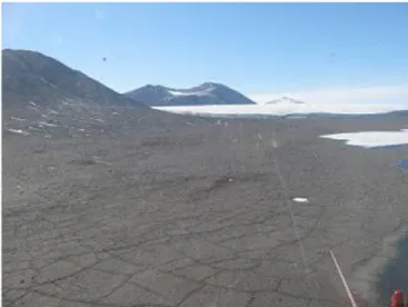
Polygonal ground

One of the most common geomorphic features associated with permafrost is the relief pattern on the surface of the ground, usually called “polygonal ground”, or “tundra polygons”. This pattern appears with the formation of a network of shallow troughs delineating 3 to 30 m diameter polygons and occurs as the result of winter freezing and spring thawing. In winter, the soil becomes brittle and cracks due to the contraction in response to cold temperatures. In spring, meltwater fills the cracks and consequently freezes forming ice wedges (Dick, 2012). Season after season, the cracks and ice wedges increase in diameter and depth. From the air perspective, the tundra will show a pattern of cracks looking like honeycombs (Figure 3). In many areas of the continuous permafrost zone, drainage follows the troughs of the tops of the ice wedges forming the polygons; and at ice wedge junctions, melting may occur to form small pools. The joining of these small pools by a stream causes what is known as beaded

drainage (Figure 4). Such drainage evidences the presence of perennially frozen, fine-grained

sediments cut by ice wedges (Péwé, 1979).

Figure 3. Helicopter view from of the polygonal ground in the F6 camp on Lake Fryxell in Taylor Valley

(27)

9

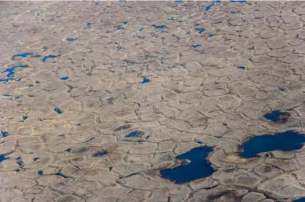
Figure 4. Tundra polygons and beaded drainage on the north slope in the Arctic National Wildlife Refuge,

Alaska (Shaw, 2015).

• Thermokarst

The thawing of permafrost creates thermokarst topography, an irregular surface containing mounds, sinkholes, caves, tunnels and steep-walled ravines resulting from the melting of ground ice (Péwé, 1979).

Thawed depressions filled with water are known as thermokarst lakes (Figure 5) and are widespread in permafrost regions, especially in those underlain with permanently frozen silt. They can appear on hillsides or even on hilltops and are good indicators of ice-rich permafrost (Péwé, 1979).

Figure 5. Circular thermokarst lakes in peatlands, Hudson Bay Lowlands,

(28)

10 • Pingos

Other landforms linked to permafrost are pingos, which are ice-cored circular or elliptical hills of frozen sediments or bedrock. Pingos can reach dimensions up to 60 m high and 450 m in diameter. They can occur in the continuous permafrost zone, especially in the tundra. They are much less outstanding in the forested area of the discontinuous permafrost zone. Frequently they are cracked on top with summit craters formed by thawing massive ice (Figure 6) (Péwé, 1979).

Figure 6. Open system pingo in upper Eskerdalen, 35 km east of Longyearbyen, Svalbard, Norway. Photo:

Hanne Christiansen (Ingólfsson, 2008).

• Patterned ground

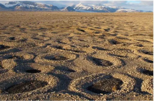
Intense and repeated freezing and thawing throughout the year produces small-scale patterned ground. This phenomenon tends to stir and sort granular sediments, forming circles, stone nets, and polygons a few centimetres to 6 m in diameter (Figure 7) (Péwé, 1979). These features require a cold climate besides a ground composed by some fine-grained soils and high water content, but they do not necessarily need to be underlained by permafrost. However, permafrost constitutes a non-permeable substrate that keeps the soil water content available for freezing.

(29)

11

Figure 7. Sorted circles 2–3 m in diameter with gravel borders about 0.25 m high, Broggerhalvoya, NW

Spitsbergen (Hallet, 2013).

•

Solifluction

In areas underlain by an impermeable layer of seasonal frozen ground, the active layer is often saturated with water and becomes easily deformable. The progressive downslope movement of water saturated soil under the action of gravity and frost is called solifluction. This material moves in a semifluid condition and results in lobe-like and sheet-like flows of soil on slopes. The pattern formed on the ground because of this phenomenon is known as solifluction lobes

and sheets (Figure 8). An outstanding feature of solifluction is the mass transport of material

over low-angle slopes (Péwé, 1979).

(30)

12

1.3 Global and regional impacts of permafrost dynamics in a global

warming scenario

Permafrost and its dynamics are important components of the cryosphere as well as the Earth system as a whole. These dynamics interact with ecosystems and climate on various spatial and temporal scales.

Climate change is expected to have considerable effects above and below ground climate being the main reason for the modifications of the structure and distribution of permafrost (Schaefer, 2014). The combination of complex permafrost-ecosystem-climate interactions in a warming world could exacerbate the overall impacts of permafrost dynamics to the Earth system. The feedbacks resulting from these interactions range from local impacts on ecosystem processes, to complex influences on global scale biogeochemical cycling (Grosse et al., 2016).

1.3.1 GLOBAL IMPACTS OF PERMAFROST DYNAMICS

Global concerns on permafrost dynamics are related with the Earth’s carbon cycle. The most recent studies investigating the permafrost carbon pool size estimate that 1035 Gt of carbon is stored in the frozen organic soil in the northern circumpolar permafrost region (Schuur, 2015). The rest of Earth’s biomes, excluding the Arctic and boreal regions, are thought to contain around 2,050 Gt carbon. This pool may cause climate impacts at the global scale upon thaw and mobilization (Schuur et al., 2015). This is, if permafrost thaws where carbon pools are present, the stored carbon may be released in the form of carbon dioxide and methane, which are powerful greenhouse gases that would again contribute to an increased rate of warming constituting a feedback loop (Schaefer, 2014).

In Antarctica, permafrost shows lower carbon content and its contribution to greenhouse gas fluxes is minor at a global scale (Turner et al., 2009). The contribution of Antarctic permafrost might have even the opposite effect than Arctic permafrost because recently deglaciated terrain, or areas with a thickening active layer, may function in the intermediate to long-term as carbon sinks due to increased biomass from colonization by new plant species and microbial communities (Vieira et al., 2010)

(31)

13

1.3.2 REGIONAL IMPACTS OF PERMAFROST DYNAMICS

Local and regional consequences of changes in permafrost dynamics vary from changes in the ecosystem’s vegetation, fauna, hydrology and terrain, to costly infrastructural damages and economic costs (Grosse et al., 2016).

• Ecosystem disturbances: vegetation, hydrology, and fauna.

Plant life can be supported only within the active layer since growth can occur only in soil that is fully thawed for some part of the year. Therefore, plant growth and rooting zones are largely restricted to the active layer, since roots cannot penetrate the frozen ground beneath (Ullrich, 2016). Because of this, the dominant ecosystems in permafrost regions are boreal forests and tundra. Sedges, shrubs, mosses and lichens dominate tundra vegetation while evergreen spruce, fir and pine, as well as the deciduous larch or tamarack dominate boreal forests.

In the Arctic, boreal forests occur in the southern regions and tundra up in the north (Schaefer et al., 2012). The tundra in Antarctica occurs mainly close to the coastline, while cold deserts occur in the mainland and at high altitude (Lopez-Terril, 2014). In mountainous permafrost regions, forests dominate at lower elevations and tundra at higher elevations (Schaefer et al., 2012).

Regarding the hydrology and fauna in permafrost regions, permafrost is impermeable to water, so rain and melt water accumulate on the surface forming numerous lakes and wetlands. These lakes and wetlands are favourable to migratory birds from around the world, which use them as summer breeding grounds (Schaefer et al., 2012). However, permafrost constitutes also limitations for fauna requiring subsurface homes, as building dens and burrows in the frozen ground beneath the surface is often harsh. Other species dependent on plants and animals, such as bacteria, have their habitat constrained by the permafrost as well. One gram of soil from the active layer may include more than one billion bacteria cells. However, the number of bacteria in permafrost soil is much lower varying typically from 1 to 1000 million per gram of soil (Hansen, 2017). Permafrost degradation may disturb ecosystems and change species composition, modifying wildlife habitats and migration (Schaefer, 2012).

(32)

14

The main ecosystem factor affected by degrading permafrost will be the local hydrology, which will suffer changes with wetlands and lakes forming in continuous permafrost and disappearing in discontinuous permafrost (Smith et al., 2005).

• Terrain disturbances: Topography and slope stability

Climate change is expected to increase erosion rates along the Arctic and Antarctic coastline (Schaefer, 2012). As much of the structural stability in mountain ranges can be attributed to glaciers and permafrost, thawing permafrost in steep mountain terrain increases the risk of rock falls and landslides (Harris et al. 2001). Talus and rock faces cemented together by ice in mountainous permafrost zones can form rock glaciers that creep downhill at velocities of centimetres to several meters per year (Figure 9).

Figure 9. Rock and talus debris flowing downhill in a rock glacier near McCarthy, Alaska

(photo: Isabelle Gärtner-Roer) (Schaefer et al., 2012).

If temperatures increase, ice on the permafrost will deform more easily of even thaw, resulting in an increase of collapse risk, landslides and rock glacier flow (Schaefer et al., 2012).

• Infrastructure:

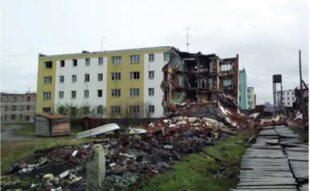
Thawing permafrost is structurally weak, resulting in foundational settling that can damage or even destroy infrastructure as buildings, roads, pipelines, railways, and power lines (Figure 10). Infrastructure failure can have dramatic environmental consequences, as seen in the 1994 breakdown of the pipeline of the Vozei oilfield in

(33)

15

Northern Russia, which resulted in a spill of 160,000 tons of oil, the world’s largest terrestrial oil spill (Schaefer et al., 2012).

Permafrost regions in the North Hemisphere are more vulnerable to damage as it counts with more infrastructure and population than the South Hemisphere permafrost regions. However, the effect of climate change on subsidence on Antarctica is of major concern, particularly in coastal areas with abundant ground ice, since despite the small total area of infrastructure in Antarctica, financial investments are substantial (Vieira et al., 2010).

Figure 10. Irregular settling due to permafrost thaw destroyed this apartment building in Cherski, Siberia

(photo: Vladimir Romanovsky, in Schaefer et al., 2012).

The impacts of the permafrost-ecosystem-climate feedbacks mentioned above have significantly raised the awareness for this component of Earth’s cryosphere in the view of stakeholders, decision makers, and the public over the last few years (Grosse et al., 2016).

Moreover, although widespread changes to permafrost usually take centuries, the

Intergovernmental Panel on Climate Change (IPCC) report estimates that “by the mid-21st

century the Arctic and alpine air temperatures will increase at roughly twice the global rate and the area of permafrost in the Northern Hemisphere will decline by 20-35%” (IPCC, 2007). Additionally, the United Nations Environmental Programme (UNEP, 2012) suggests the depth of thawing could increase by 30-50% by the year 2080.

In recognition of this importance, permafrost has been added as an Essential Climate Variable (ECV) in the Global Climate Observing System (GCOS) of the World Meteorological

(34)

16

Organization (WMO). Consequently, permafrost now requires broad-scale research and

systematic observations to support the IPCC and United Nations Framework Convention on

Climate Change (UNFCC) in their assessments of the state of the global climate system and

its variability (Grosse et al., 2016).

To understand the status and dynamics of permafrost, the monitoring of ground temperature and active layer thickness are needed. Other observations include sample drilling, remote sensing to detect changes in land surface characteristics and measurements of surface subsidence or heave (Schaefer et al., 2012).

1.4 Global Permafrost Monitoring

The creation of national permafrost monitoring networks was considered by the IPCC as one of the key steps to understand the potential impacts of permafrost dynamics in a climate-changing world affected by global warming (Grosse et al., 2016).

Currently, there are two global networks to monitor permafrost: the Thermal State of Permafrost (TSP) network, which coordinates measurements of permafrost temperature; and the Circumpolar Active Layer Monitoring (CALM) network, which coordinates measurements of active layer thickness in both polar regions as shown in Figure 11.

(35)

17

Figure 11. Circumpolar Active Layer Monitoring (CALM) network and Thermal State of Permafrost (TSP)

network distribution (Schaefer, 2014).

The TSP and CALM networks are the two components of the Global Terrestrial Network for Permafrost (GTN-P). The GTN-P was initiated by the International Permafrost Association (IPA) to organize and manage a global network of permafrost observations for detecting, monitoring and predicting climate change, and was implemented under the GCOS and its associated organizations. The IPA currently coordinates international development and operation of the TSP and CALM networks for the GTN-P (Schaefer et al., 2012).

The TSP network measures permafrost temperature using boreholes. Boreholes vary in depth from a few meters to a hundred meters and deeper, with a string of temperature sensors at multiple depths. Newer boreholes are automated, but manually lowering a single sensor probe down a borehole to measure temperature is still common. The oldest boreholes have operated since the middle of the 20th century, with several decades of permafrost temperature observations. The TSP network includes approximately 1357 boreholes mostly located in the Arctic, also includes boreholes in the European Alps, Antarctica and the Qinghai-Tibetan Plateau (GNT-P, 2018).

The CALM network measures active layer thickness or maximum annual thaw either mechanically using a probe, or electronically with a vertical sequence of temperature sensors. The probe is a metal rod sunk into the ground until it hits the hard top of permafrost. The active layer depth is measured on the rod and recorded. To account for high spatial variability,

(36)

18

researchers generally probe the active layer on a specified 1 km or 100 m grid. A 252-sites network presently exists under the CALM Network (GNT-P, 2018), some of which have been measuring active layer thickness since the 1990s (Schaefer et al., 2012).

Most stations in TSP and CALM are nationally or regionally funded and operated by independent research teams. TSP and CALM coverage are limited because installation and maintenance costs restrict sites to regions with reasonable access by truck, plane or boat. The research teams in the GTN-P have made tremendous progress, but evaluation of overall permafrost status in a region or country is still very difficult because of the non-standard observations and limited coverage of the TSP and CALM networks, due to a limited and irregular funding (Schaefer et al., 2012). Moreover, international collaboration on data collection and analysis is still a great challenge to overcome in this advancing scientific problem of global concern. The willingness of scientists to share data and to participate in data management strategies is as well a crucial requirement for scientific advancement (Papale et al., 2012)

Specially during the International Polar Year (IPY) in 2007-08, the Antarctic region received great efforts to increase the spatial coverage of the existing permafrost-monitoring network and installing boreholes deeper than the depth of ZAA (Figure 12) all around the continent (Vieira et al., 2010). About 350 new boreholes for temperature monitoring were established globally and a considerable number of active layer depth observations were collected during this year (Biskaborn et al., 2015). Meteorological stations were as well installed close to some boreholes in order to evaluate ground–atmosphere coupling (Vieira et al., 2010).

Efforts of the IPA and the GTN- P at the end of the IPY resulted in reports on the thermal state of permafrost in high latitudes and high altitudes which were called the “IPA snapshot” and published in a special issue of the journal Permafrost and Periglacial Processes (Christiansen et al., 2010; Romanovsky et al., 2010a; Smith et al., 2010; Vieira et al., 2010; Zhao et al., 2010).