Distributions of Topological Observables in Inclusive Three- and Four-Jet Events in pp Collisions at sqrt(s) = 7 TeV

(1)

EUROPEAN ORGANIZATION FOR NUCLEAR RESEARCH (CERN)

CERN-PH-EP/2013-037 2015/07/14

CMS-QCD-11-006

Distributions of topological observables in inclusive

three-and four-jet events in pp collisions at

√

s

=

7 TeV

The CMS Collaboration

∗

Abstract

This paper presents distributions of topological observables in inclusive three- and four-jet events produced in pp collisions at a centre-of-mass energy of 7 TeV with a data sample collected by the CMS experiment corresponding to a luminosity of

5.1 fb−1. The distributions are corrected for detector effects, and compared with

sev-eral event generators based on two- and multi-parton matrix elements at leading

or-der. Among the considered calculations, MADGRAPH interfaced withPYTHIA6

dis-plays the overall best agreement with data.

Published in the European Physical Journal C as doi:10.1140/epjc/s10052-015-3491-9.

c

2015 CERN for the benefit of the CMS Collaboration. CC-BY-3.0 license ∗_{See Appendix A for the list of collaboration members}

(2)

(3)

1

1 Introduction

In proton-proton collisions at the LHC, interactions take place between the partons of the collid-ing protons. The scattered partons from hard collisions fragment and hadronize into collimated

groups of particles called jets. The study of jets with high transverse momentum (pT) provides

a test of the predictions from quantum chromodynamics (QCD) and deviations from these pre-dictions can be used to look for physics beyond the standard model. While parton scattering is an elementary QCD process that can be calculated from first principles, predictions of jet distri-butions require an accurate hadronization model. In this paper, several hadronization models are examined.

High-pT parton production is described by perturbative QCD (pQCD) in terms of the

scat-tering cross section convolved with a parton distribution function (PDF) for each parton that parametrizes the momentum distribution of partons within the proton. The hard-scattering

cross section itself can be written as an expansion in the strong coupling constant αs. The

lead-ing term in this expansion corresponds to the emission of two partons. The next term includes diagrams where an additional parton is present in the final state as a result of hard-gluon

ra-diation (e.g. gg→ ggg). Cross sections for such processes diverge when any of the three

par-tons becomes soft or when two of the parpar-tons become collinear. Finally, pQCD predicts three

classes of four-jet events that correspond to the processes qq/gg→qqgg, qq/gg → qqqq and

qg→qggg/qqqg, where q stands for both quarks and anti-quarks. Processes with two or more

gluons in the final state receive a contribution from the triple-gluon vertex, a consequence of the non-Abelian structure of QCD.

We are studying distributions of topological variables, which are sensitive to QCD color fac-tors, the spin structure of gluons, and hadronization models. These topological variables were studied widely in the earlier LEP [1, 2] and the Tevatron [3, 4] experiments and help to validate theoretical models implemented in various Monte Carlo (MC) event generators.

The distributions of multijet variables are sensitive to the treatment of the higher-order pro-cesses and approximations involved. Many MC event generators make use of leading order

(LO) matrix elements (ME) in the primary 2→2 process. A good agreement between the

mea-surements and MC predictions can establish the validity of the treatment of higher-order ef-fects, and any large deviation may lead to large systematic uncertainties in searches for new physics.

The multijet observables presented here are based on hadronic events from 7 TeV pp collision

data recorded with the CMS detector corresponding to an integrated luminosity of 5.1 fb−1. The

kinematic and angular properties of these events are computed from the jet momentum four-vectors. Unfolding techniques are used to correct for the effects of the detector resolution and efficiency. Systematic uncertainties resulting from the limited knowledge of the jet energy scale (JES), jet energy and angular resolution (JER), unfolding, and event selection are estimated, and the unfolded distributions are compared with predictions of several QCD-based MC models. In this paper, the CMS detector is briefly described in Section 2. Sections 3 and 4 summarize the MC models used and the variables studied in this paper. Event selection and measurements are described in Sections 5 and 6, respectively. The correction of the distributions due to de-tector effects is discussed in Section 7. Sections 8 and 9 describe the estimation of systematic uncertainties and the final results. The overall summary is given in Section 10.

(4)

2 3 Monte Carlo models

2 The CMS detector

The central feature of the CMS apparatus is a superconducting solenoid of 6 m internal di-ameter, providing a magnetic field of 3.8 T. Within the field volume are a silicon pixel and strip tracker, a lead tungstate crystal electromagnetic calorimeter (ECAL), and a brass and scintillator hadron calorimeter (HCAL), each composed of a barrel and two endcap sections. Muons are measured in gas-ionization detectors embedded in the steel flux-return yoke out-side the solenoid. Extensive forward calorimetry complements the coverage provided by the barrel and endcap detectors. The barrel and endcap calorimeters cover a pseudorapidity

re-gion −3.0 < η < 3.0. Pseudorapidity is defined as η = −ln tan[θ/2], where θ is the polar

angle. The transition between barrel and endcaps happens at|η| = 1.479 for the ECAL and

|η| = 1.15 for the HCAL. The first level (L1) of the CMS trigger system, composed of custom

hardware processors, uses information from the calorimeters and muon detectors to select the most interesting events in a fixed time interval of less than 4 µs. The high-level trigger (HLT) processor farm further decreases the event rate from around 100 kHz to around 400 Hz before data storage. A more detailed description of the CMS detector, together with a definition of the coordinate system used and the relevant kinematic variables, can be found in Ref. [5].

3 Monte Carlo models

The MC event generators rely on models using modified LO QCD calculations. The elementary hard process between the partons is computed at LO. The parton shower (PS), used to simulate higher-order processes, follows an ordering principle motivated by QCD. Nevertheless, the parton shower models can differ in the ordering of emissions and the event generators can also have different treatments of beam remnants and multiple interactions.

ThePYTHIA6.4.26 [6] event generator uses a PS model to simulate higher-order processes [7–9]

after the LO ME from pQCD calculations. The PS model, ordered by the pT of the emissions,

provides a good description of event shapes when the emitted partons are close in phase space. Events are generated with the Z2 tune [10] for the underlying event. This tune is identical to the Z1 tune [11], except that it uses CTEQ6L1 [12] PDFs. The partons are hadronized (process of converting the partons into measured particles) using the Lund string model [13, 14]. The PYTHIA8.153 [15] event generator also uses a PS model with the successive emissions of

partons ordered in pT and the Lund string model for hadronization. The main difference

be-tween the twoPYTHIAversions is the description of multiparton interactions (MPI). InPYTHIA8,

initial state radiation (ISR), final state radiation (FSR), and MPI are interleaved in the pT

order-ing, while inPYTHIA6, only ISR and FSR are interleaved. The TUNE4C [16] is used with this

generator. This tune uses CTEQ6L1 PDFs with parameters using CDF as well as early LHC measurements.

The HERWIG++ 2.4.2 [17] TUNE23 [18] program takes the LO ME and simulates a PS using the coherent branching algorithm with angular ordering [19] of the showers. The partons are hadronized in this model using a cluster model [20] and the underlying event is simulated using the eikonal multiple partonic scattering model.

In the case of MADGRAPH5.1.5.7 [21], multiparton final states are also computed at tree level.

The parton shower and nonperturbative parts for MADGRAPH 5.1.5.7 simulation sample is

handled byPYTHIA 6.4.26 with Z2 tune. The MLM matching procedure [22] is used to avoid

double counting between the ME and the PS. The MADGRAPHsamples are created in four bins

(5)

3

been studied in detail and has been validated using inclusive jet pTdistributions. Several

sam-ples are generated using different matching parameters and are used in estimating systematic uncertainty in the theoretical prediction.

These MC programs are the most commonly used models to describe multi-partonic final states and are normally used to describe QCD background in searches within CMS. The events pro-duced from these models are simulated using a CMS detector simulation program based on

GEANT4 [23] and reconstructed with the same program used for the data. These MC events

are used for the comparison with the measurements as well as to correct the distributions for detector effects.

4 Definition of variables

4.1 Three-jet variables

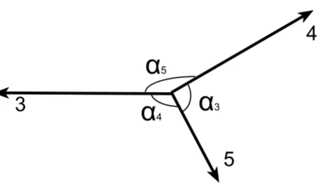
The topological variables used in this study are defined in the parton or jet centre-of-mass (CM) system. The topological properties of the three-parton final state in the CM system can be described in terms of five variables [3]. Three of the variables reflect partition of the CM energy among the three final-state partons. There are three angles, which define the spatial orientation in the plane containing the three partons, but only two are independent.

3

4

5 α

3

α

4

α

5

Figure 1: Illustration of the three-jet variables in the process 1+2→3+4+5. The scaled energies

are related to the angles (αi) among the jets for massless parton.

It is convenient to introduce the notation 1+2→3+4+5 for the three-parton process. Here,

num-bers 1 and 2 refer to incoming partons while the numnum-bers 3, 4, and 5 label the outgoing partons

in a descending order in energies in the parton CM frame, i.e. E3> E4> E5(Fig. 1). The

final-state parton energy is an obvious choice for the topological variable for the three-parton final

state. For simplicity, Ei(i =3, 4, 5) is often replaced by the scaled variable xi(i=3, 4, 5), which

is defined by xi = 2Ei/

√

ˆs345, where

√

ˆs345 is the CM energy of the hard-scattering process. It

is also referred to as the mass of the three-parton system, and by definition,

x3+x4+x5 =2. (1)

The internal structure of the three-parton final state is determined by any two scaled parton energies. The third one is calculated using Equation 1. It needs two angular variables which fix the event orientation. In total, five independent kinematic variables are needed to describe the topological properties of the three-parton final state. In this analysis, however, the study is

(6)

4 4 Definition of variables

4.2 Four-jet variables

To define a four-parton final state in its CM frame, eight independent parameters are needed. Two of these define the overall event orientation, while the other six fix the internal structure of the four-parton system. In contrast to the three-parton final state, there is no simple relationship between the scaled parton energies and the opening angles between partons. Consequently, the choice of topological variables is less obvious in this case. Variables are defined here in a way similar to those investigated for the three-parton final state. The four partons are ordered in descending energy in the parton CM frame and labeled from 3 to 6. The variables include the scaled energies and the polar angles of the four partons with respect to the beams.

In addition to the four-parton CM energy or the mass of the four-parton system (√ˆs3456), two

angular distributions characterizing the orientation of event planes are investigated. One of

these is the Bengtsson–Zerwas angle (χBZ) [24] defined as the angle between the plane

contain-ing the two leadcontain-ing jets and the plane containcontain-ing the two nonleadcontain-ing jets:

cos χBZ =

(~p3× ~p4) · (~p5× ~p6)

|~p3× ~p4||~p5× ~p6|

. (2)

The second variable is the cosine of the Nachtmann–Reiter angle (cos θNR) [25] defined as the

angle between the momentum vector differences of the two leading jets and the two nonleading jets:

cos θNR =

(~p3− ~p4) · (~p5− ~p6)

|~p3− ~p4||~p5− ~p6|

. (3)

Figure 2 illustrates the definitions of χBZ and θNR variables. Historically, χBZ and θNR were

proposed for e+_e−_{collisions to study gluon self-coupling. Their interpretation in pp collisions}

is more complicated, but the variables can be used as a tool for studying the internal structure of the four-jet events.

3

4

5

6 χ

BZ

θ

NR

3

4

5

6

Figure 2: Illustration of the Bengtsson–Zerwas angle (χBZ) and the Nachtmann–Reiter angle

(θNR) definitions for the four-jet events. The left figure shows the Bengtsson–Zerwas angle,

which is the angle between the plane containing the two leading jets and the plane containing the two nonleading jets. The right figure shows the Nachtmann–Reiter angle, which is the angle between the momentum vector differences of the two leading jets and the two nonleading jets.

(7)

5

5 Data samples and event selection

Jets are reconstructed from particle-flow (PF) objects [26, 27] using the anti-kT clustering

al-gorithm [28] with the distance parameter R = 0.5, as calculated with FASTJET2.0 [29]. The

PF algorithm utilizes the best energy measurements of each particle candidate from the most suitable combination of the detector components. A cluster is formed from all the particle-flow candidates that satisfy the chosen distance parameter. The four-momentum of the jet is then defined as the sum of four-momenta of the corresponding particle-flow candidates, which results in jets with nonzero mass.

The JES correction applied to jets used in this analysis is based on high-pT jet events

gener-ated byPYTHIA6 and then simulated using GEANT4, and in situ measurements with dijet and

photon+jet events [30]. An average of ten minimum bias interactions occur in each pp bunch crossing (pileup), and this requires an additional correction to remove the extra energy

de-posited by these pileup events. The size of the correction depends on the pT and η of the jet.

The correction appears as a multiplicative factor to the jet energy, and is typically less than 1.2 and approximately uniform in η.

Events passing single-jet HLT requirements are used in this analysis. These triggers require jets

reconstructed from calorimetric information with the anti-kTclustering algorithm and with

en-ergy corrections applied. Jets are ordered in decreasing jet pT, and the leading jet pTis required

to be above a certain threshold. As offline jets are reconstructed with the PF algorithm, this may result in a trigger not being fully efficient near the threshold. Trigger efficiencies are studied as

a function of the leading jet pTfor all trigger thresholds. Values of the leading jet pT, where the

trigger efficiency is determined to be larger than 99%, are listed in Table 1. It also summarizes the prescale factors and the effective integrated luminosities collected using the different HLT thresholds.

Table 1: Prescales, integrated luminosity and offline pTthreshold of the leading jet for different

trigger paths. The terminology for Level 1 (L1) triggers as well as HLT includes the jet pT

threshold (in GeV) applicable to the trigger.

Period HLT HLT60 HLT110 HLT190 HLT240 HLT370

L1 SingleJet36 SingleJet68 SingleJet92 SingleJet92 SingleJet92/

SingleJet128 2011A L1 prescale 1–300 1–10 1 1 1 HLT prescale 15–180 1–5000 1–60 1–24 1 R L( pb−1) 0.29 6.16 114.7 392.2 2328 2011B L1 prescale 50–400 1–20 1–10 1 1 HLT prescale 80–84 80–1000 10–100 4–30 1 R L( pb−1) 0.12 1.12 40.2 136.0 2767 Overall R L( pb−1) 0.41 7.29 154.8 528.2 5096

pTthreshold 110 GeV 190 GeV 300 GeV 360 GeV 500 GeV

Jets are selected with restrictive criteria on the neutral energy fractions (both electromagnetic

and hadronic components), and all the jets are required to have pT > 50 GeV and absolute

rapidity, (y = (1/2)ln[(E+pz)/(E− pz)]), |y| ≤ 2.5. The jet with the highest pT is required

to be above a threshold as given by the requirement from the trigger turn-on curve. To avoid

overlap of events from two different HLT paths, the pT of the leading jet is also required to be

less than an upper value. The overall criteria are summarized in Table 2. Though data from all

the five trigger paths are studied, figures from two representative trigger paths (the highest pT

(8)

6 7 Corrections for detector effects

Table 2: Threshold of the leading jet pTfor different HLT paths. This paper shows results from

two representative trigger paths HLT110 and HLT370.

HLT HLT60 HLT110 HLT190 HLT240 HLT370

Leading jet pT (GeV) 110–190 190–300 300–360 360–500 >500

Events are selected with at least three jets passing the selection criteria as stated above. Addi-tional selection requirements are also applied to reduce backgrounds due to beam halo, cosmic rays and detector noise. The event must have at least one good reconstructed vertex [31].

Miss-ing transverse energy, Emiss_T , is required to be less than 0.3_{∑ E}T, where the summation is over

all PF jets. The quantities Emiss_T and_{∑ E}Tare obtained from negative vector sum and scalar sum

of the transverse momenta of the jets, respectively. A number of event filters [32] accept only

those events that have negligible noise in the detector. The jets are ordered in decreasing pT,

and an event with at least three (four) jets satisfying the jet selection criteria is classified as a three-jet (four-jet) event.

6 Measurements

The 4-momenta of all the jets in the three- or four-jet event category are transformed into the CM frame of the three- or four-jet system. The jets are then ordered in decreasing energy. The three- and four-jet variables as described in Section 4 are then calculated from the kinematic and angular information of the jets. Since detector resolution varies over the potential kinematic ranges, variable bin widths are adopted for the jet masses and the scaled jet energies, while for angular variables constant bin widths are used.

6.1 Detector-level distributions

The measured distributions of the three- and four-jet variables are compared with predictions

from two MC generators (PYTHIA6 and MADGRAPH+PYTHIA6), simulated using the identical

detector condition as that in the data. The identical pileup condition is obtained by reweighting the MC simulation to match the spectrum of pileup interactions observed in the data. The size of the reweighting correction is typically less than 1%. The agreement between the data and the MC predictions is reasonable, so these MC generators are used to correct the measured distributions.

Figures 3 and 4 show the normalized three- and four-jet mass distributions. The data are

com-pared with two different MC programs: PYTHIA6 and MADGRAPH+PYTHIA6, each with two

different HLTs with pT thresholds above 110 and 370 GeV. As can be seen from the figures,

there is agreement within a few percent between the data and the predictions of these two sim-ulations. The difference between the predictions and the data varies typically from 4% to 10%. However, there is a systematic deviation observed at high masses where the simulations are higher than the data.

7 Corrections for detector effects

Multijet variables obtained from MC samples may differ from data because of the detector res-olution and acceptance. Before comparisons with other experiments or theoretical predictions can be made, detector effects are unfolded into distributions at the final-state particle level. The basic component of the unfolding is the response function, where experimental observables are expressed as a function of theoretical observables. For simplicity, observables are taken in

(9)

7 400 600 800 1000 1200 1400 1600 1800 2000 ) -1 (GeV dm dN . N 1 -5 10 -4 10 -3 10 -2

10 Madgraph + Pythia6 TuneZ2 Pythia6 TuneZ2 Data

CMS

Three-jet mass (GeV)

500 1000 1500 2000

Data

Pythia6 0.5

1 1.5

Three-jet mass (GeV) 400 600 800 1000 1200 1400 1600 1800 2000 Data Madgraph 0.5 1 1.5 (7 TeV) -1 5.1 fb < 300 GeV T

190 GeV < Leading jet p (a) 1000 1500 2000 2500 3000 3500 ) -1 (GeV dm dN . N 1 -5 10 -4 10 -3 10 -2

CMS

1000 2000 3000

Data

Pythia6 0.5

1 1.5

Three-jet mass (GeV) 1000 1500 2000 2500 3000 3500 Data Madgraph 0.5 1 1.5 (7 TeV) -1 5.1 fb > 500 GeV T Leading jet p (b)

Figure 3: The upper panels display the normalized distributions of the reconstructed three-jet

mass for events where the most forward jet has |y| < 2.5. Figures differ by pT ranges of the

leading jet: 190–300 GeV (a), and above 500 GeV (b) for data (before correction due to detector effects) and predictions from MC generators. The bottom panel of each plot shows the ratio of MC predictions to the data. The data are shown with only statistical uncertainty.

500 1000 1500 2000 2500 ) -1 (GeV dm dN . N 1 -5 10 -4 10 -3 10 -2

CMS

Four-jet mass (GeV)

500 1000 1500 2000 2500

Data

Pythia6 0.5

1 1.5

Four-jet mass (GeV) 500 1000 1500 2000 2500 Data Madgraph 0.5 1 1.5 (7 TeV) -1 5.1 fb < 300 GeV T

190 GeV < Leading jet p (a) 1000 1500 2000 2500 3000 3500 ) -1 (GeV dm dN . N 1 -5 10 -4 10 -3 10 -2

CMS

Four-jet mass (GeV)

1000 2000 3000

Data

Pythia6 0.5

1 1.5

Four-jet mass (GeV) 1000 1500 2000 2500 3000 3500 Data Madgraph 0.5 1 1.5 (7 TeV) -1 5.1 fb > 500 GeV T Leading jet p (b)

Figure 4: The upper panels display the normalized distributions of the reconstructed four-jet

mass for events where the most forward jet has|y| < 2.5. The other explanations are the same

(10)

8 8 Systematic uncertainties

discrete sets, and the response function is replaced by a response matrix. The observed distri-bution is then unfolded with the inverse of response matrix to obtain a distridistri-bution corrected for detector effects. Matrix inversion has potential complications, because it cannot handle large statistical fluctuations and the matrix itself could be singular. Instead, we use the RooUn-fold package [33] with the D’Agostini iterative method [34] as the default algorithm and the singular value decomposition method [35] for cross-checks.

The default response matrix is obtained using thePYTHIA6 event generator. Statistical

uncer-tainties are estimated from the square root of the covariance matrix obtained from a variation of the results generated by simulated experiments.

The corrections for detector resolution and acceptance change the shape of the three-jet mass distributions by approximately 10%, less than 5% for the scaled energy of nonleading jets, and up to 20% for the scaled energy of the leading jet. For four-jet variables, corrections applied are

of the order of 20% for the four-jet mass, 10% for χBZ, and less than 5% for cos θNR.

8 Systematic uncertainties

The leading sources of systematic uncertainty are due to the JES, the JER, and the model depen-dence of corrections to the data. The distributions are presented in this analysis as normalized distributions, thus the absolute scale uncertainty of energy measurement does not play a sig-nificant role. There are insigsig-nificant contributions due to resolution of y. The main contribution of JES or JER to the uncertainty in the measurements is due to the migration of events from one category of jet multiplicity to the other.

The effect of pileup in the measured distributions has been studied as a function of the number of reconstructed vertices in the event. None of the variables show any significant dependence on the pileup condition, so systematic uncertainty due to pileup can be neglected.

8.1 Jet energy scale

One of the dominant sources of systematic uncertainty is due to the jet energy scale corrections.

The JES uncertainty has been estimated to be 2–2.5% for PF jets [30], depending on the jet pT

and η. In order to map this uncertainty to the multijet variables, all jets in the selected events are systematically shifted by the respective uncertainties, and a new set of values for the multijet variables is calculated. This causes a migration of events from an event category of a given jet multiplicity to a different jet multiplicity. The migration could be as high as 20% for some of the event categories. The corresponding distributions are then unfolded using the standard procedure as described in Section 7. The difference of these values from the central unfolded results is a measure of the uncertainty owing to the JES.

Uncertainties owing to the JES are found to be between 0.2–5.5% in the three-jet mass, and 0.3– 10% in the four-jet mass. The systematic uncertainties are the largest at both ends of the mass spectra. The systematic uncertainties in scaled energy are between 0.1% and 2.0%, and those in angular variables are in the range 0.1–3.0%. There is a small increase in the uncertainty for distributions where there is at least one jet in the endcap region of the detector.

8.2 Jet energy resolution

The JER is measured in data using the pTbalance in dijet events [36]. Based on these

measure-ments, the resolution effects are corrected using simulated events. To study the effect of the difference between the simulated and the measured resolution, several sets of unfolded

(11)

distri-8.3 Model dependence in unfolding 9

butions are obtained using response matrices from the default resolution matrix and changing the jet resolution within its estimated uncertainty. Alternatively, the response matrix is con-structed by convolving the generator level distribution with the measured resolution. The mea-sured distribution is unfolded by this response matrix vis-a-vis the response matrix determined

using fully simulated sample ofPYTHIA6 events. These two estimates provide independent

de-scriptions of the detector modeling and the difference is used as a measure of the systematic uncertainty due to detector performance. Position resolution affects the measurement of the jet direction, and it is estimated using simulated multijet events and validated with data.

Uncertainties owing to the JER are found to be between 0.1–10% in the three-jet mass, 0.3–15% in the four-jet mass, 0.1–10% in the scaled jet energies and 0.2–8.2% in the angular variables.

8.3 Model dependence in unfolding

Unfolded distributions are obtained using two different response matrices derived fromPYTHIA6

and from MADGRAPH+PYTHIA6 simulations. The difference in the unfolded values, due to the

choice of response functions, gives a measure of the systematic uncertainty. The uncertainties are at the level of 0.1–6.0% in the three-jet mass, 0.1–3.0% in the scaled energy distributions of the three-jet variables, 0.1–8.0% in the four-jet mass and 0.1–6.2% in the angular variables in the four-jet samples. The uncertainties in the scaled jet energy increases by a few percent for the

samples with lower values of leading jet pT.

Unfolding has been carried out usingPYTHIA6 and MADGRAPH+PYTHIA6 samples, which has

the same hadronization model. To test the effects of different hadronization models, MC

sam-ples from HERWIG++, which provides a different PS and hadronization approach, are used.

However, the simulated event sample generated using HERWIG++ is statistically inadequate

to be used in a complete unfolding procedure. The difference between bin-by-bin correction

factors obtained with PYTHIA6 and HERWIG++ is found to be somewhat larger than the

un-certainty due to the difference in the unfolding matrices: 0.1–12% in the scaled energy dis-tributions of three-jet variables, 0.1–7.7% in the angular variables in the four-jet samples and 0.1–11.6% in the jet masses. The larger values from the two estimates are chosen as the system-atic uncertainties due to unfolding.

8.4 Event selection

Jet candidates are required to pass certain criteria [37] designed to reduce unwanted detector effects. This analysis uses jets identified with very restrictive criteria on the ratio of the energy carried by neutral to that carried by charged particles. The effect of using these criteria is tested by reevaluating the same distributions with jets selected after relaxing the selection on the fractions of the energy carried by the neutral and the charged particles. Also, the selection

on Emiss

T is changed, and the effect of this is estimated from the difference in the observed

distributions. The uncertainty due to the event selection is found to be below 0.2%.

8.5 Overall uncertainty

The first three sources mentioned above are the dominant sources of systematic uncertainty. The contributions to the uncertainty from the selection requirements and pileup effects are found to be negligible. The uncertainties are calculated for each bin of the measured distribu-tions and are added in quadrature. The overall systematic uncertainty is found to be smaller than the statistical uncertainty for most of the bins. Typical uncertainties for the six variables studied in this analysis are summarized in Table 3.

(12)

10 8 Systematic uncertainties

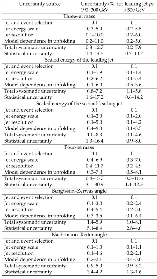
Table 3: Uncertainty ranges among the different bins in the topological distributions of the three- and four-jet variables.

Uncertainty source Uncertainty (%) for leading jet pT

190–300 GeV >500 GeV

Three-jet mass

Jet and event selection 0.1 0.1

Jet energy scale 0.3–5.0 0.2–5.5

Jet resolution 0.1–10.0 0.2–6.0

Model dependence in unfolding 0.2–11.0 0.2–5.0

Total systematic uncertainty 0.3–12.7 0.2–7.9

Statistical uncertainty 1.4–14.5 0.7–10.2

Scaled energy of the leading jet

Scaled energy of the second-leading jet

Four-jet mass

Bengtsson–Zerwas angle

Nachtmann–Reiter angle

(13)

11

9 Results

9.1 Comparison with models

The normalized differential distributions, corrected for detector effects, are plotted as a function of the three- and four-jet inclusive variables and compared with predictions from the four MC

models: PYTHIA6,PYTHIA8, MADGRAPH+PYTHIA6 andHERWIG++. The variables considered

for these comparisons are three-jet mass, scaled energies of the leading and next-to-leading jet

in the three-jet sample in the three-jet CM frame, four-jet mass, and the two angles χBZand θNR.

For the comparison plots (Figs. 5–9), the upper panel shows the data and the model predictions with the corresponding statistical uncertainty. For the data, the shaded area shows the statis-tical and systematic uncertainties added in quadrature. The lower panels in each plot show the ratio of MC prediction to the data for each model. Comparisons are made for two different

ranges of the leading jet pT: 190< pT <300 GeV and pT>500 GeV.

400 600 800 1000 1200 1400 1600 1800 2000 ) -1 (GeV dm dN . N 1 -5 10 -4 10 -3 10 -2 10 Herwig++ Tune23 Madgraph + Pythia6 TuneZ2 Pythia8 Tune4C Pythia6 TuneZ2 Unfolded data

CMS

500 1000 1500 2000

Data

Pythia6 0.5 1.0 1.5

Three-jet mass (GeV) 400 600 800 1000 1200 1400 1600 1800 2000

Data

Pythia8 0.51.0 1.5

Three-jet mass (GeV) 400 600 800 1000 1200 1400 1600 1800 2000

Data

Madgraph 0.5 1.0 1.5

Three-jet mass (GeV) 400 600 800 1000 1200 1400 1600 1800 2000 Data Herwig++ 0.5 1.0 1.5 (7 TeV) -1 5.1 fb < 300 GeV T

190 GeV < Leading jet p

(a) 1000 1500 2000 2500 3000 3500 ) -1 (GeV dm dN . N 1 -5 10 -4 10 -3 10 -2 10 Herwig++ Tune23 Madgraph + Pythia6 TuneZ2 Pythia8 Tune4C Pythia6 TuneZ2 Unfolded data

CMS

1000 2000 3000

Data

Pythia6 0.5 1.0 1.5

Three-jet mass (GeV) 1000 1500 2000 2500 3000 3500

Data

Pythia8 0.51.0 1.5

Three-jet mass (GeV) 1000 1500 2000 2500 3000 3500

Data

Three-jet mass (GeV) 1000 1500 2000 2500 3000 3500 Data Herwig++ 0.5 1.0 1.5 (7 TeV) -1 5.1 fb > 500 GeV T Leading jet p (b)

Figure 5: Distribution of the three-jet mass superposed with predictions from four MC models:

PYTHIA6, PYTHIA8, MADGRAPH+PYTHIA6, HERWIG++. The distributions are obtained from

inclusive three-jet sample with the jets restricted in the|y| region 0.0 < |y| < 2.5, and with

leading-jet pT between 190 and 300 GeV (a) or above 500 GeV (b). The data points are shown

with statistical uncertainty only and the bands indicate the statistical and systematic uncertain-ties combined in quadrature. The lower panels of each plot show the ratios of MC predictions to the data. The ratios are shown with statistical uncertainty in the data as well as in the MC, while the band shows combined statistical and systematic uncertainties.

Figure 5 shows the normalized corrected differential distribution as a function of the three-jet

mass for two ranges of the leading-jet pT. The three-jet mass distribution broadens for larger

pT thresholds. The models show varying degrees of success for the different ranges of

leading-jet pT. Most models differ from the data in the low-mass spectrum. ThePYTHIA6 simulation

provides a good description of the data in the lower pT bin, while it has a larger deviation

in the higher pT bin. The mean difference is at the level of 1.8–4.0%. Predictions from MAD

(14)

12 9 Results

worst agreement among the four models – the mean difference is at the level of 4.0–15%.

0.65 0.7 0.75 0.8 0.85 0.9 0.95 1 3 dx dN . N 1 5 10 15 20 Herwig++ Tune23 Madgraph + Pythia6 TuneZ2 Pythia8 Tune4C Pythia6 TuneZ2 Unfolded data CMS 3 x 0.7 0.8 0.9 1 Data Pythia6 0.5 1.0 1.5 3 x 0.65 0.7 0.75 0.8 0.85 0.9 0.95 1 Data Pythia8 0.51.0 1.5 3x 0.65 0.7 0.75 0.8 0.85 0.9 0.95 1 Data Madgraph 0.5 1.0 1.5 3 x 0.65 0.7 0.75 0.8 0.85 0.9 0.95 1 Data Herwig++ 0.5 1.0 1.5 (7 TeV) -1 5.1 fb < 300 GeV T

(a) 0.65 0.7 0.75 0.8 0.85 0.9 0.95 1 3 dx dN . N 1 5 10 15 20 Herwig++ Tune23 Madgraph + Pythia6 TuneZ2 Pythia8 Tune4C Pythia6 TuneZ2 Unfolded data CMS 3 x 0.7 0.8 0.9 1 Data Pythia6 0.5 1.0 1.5 3 x 0.65 0.7 0.75 0.8 0.85 0.9 0.95 1 Data Pythia8 0.51.0 1.5 3 x 0.65 0.7 0.75 0.8 0.85 0.9 0.95 1 Data Madgraph 0.5 1.0 1.5 3 x 0.65 0.7 0.75 0.8 0.85 0.9 0.95 1 Data Herwig++ 0.5 1.0 1.5 (7 TeV) -1 5.1 fb > 500 GeV T Leading jet p (b)

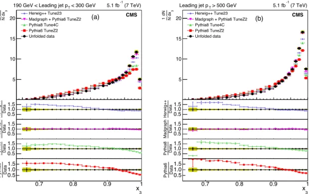
Figure 6: Corrected normalized distribution of scaled energy of the leading-jet in the inclusive three-jet sample. The other explanations are the same as Fig. 5.

Figure 6 shows the corrected normalized differential distribution as a function of the scaled leading-jet energy in the inclusive three-jet sample. The distributions peak close to 1 and the

peaks get sharper for higher leading-jet pTrange. The scaled leading-jet energy x3is expected

to follow a linear rise from 2₃ to 1 for a phase space model, which has only energy-momentum

conservation, while QCD predicts a deviation from linearity at higher values of x3. This feature

is observed in the data, particularly for higher pT bins. Only MADGRAPH+PYTHIA6 provides

a consistent description of the data. The agreement improves for the sample with leading-jet

pTabove 500 GeV. The difference between the predictions from MADGRAPH+PYTHIA6 and the

data are at the level of 3.5–6.1%.

Figure 7 shows the corrected normalized differential distribution as a function of the scaled

energy of the second-leading jet, x4, in the inclusive three-jet sample. For kinematic reasons,

x4 is expected to lie between 1/2 and 1. The distribution peaks around 0.65 for the low pT

threshold sample. The peak shifts to higher values of x4and the distribution becomes broader

for the larger pTthreshold sample. Predictions from MADGRAPH+PYTHIA6 agree with data to

within 3.1%. Predictions fromPYTHIA6 as well asPYTHIA8 deviate by as much as 10% or more

from the data. Predictions fromHERWIG++ also shows a large deviation at higher pTbins.

Figure 8 shows comparisons of the corrected normalized differential distribution as a function

of the four-jet mass for the four MC models. The distribution broadens at higher minimum pT

value. As can be seen from the figure,HERWIG++ provides the worst comparison. The average

deviations are at the level of 15% for many of the distributions, particularly for the sample with

leading-jet pTbetween 190 and 300 GeV. The level of agreement for the other three MC models

is better than 10% over the entire pTregion.

The sub-leading jets in the four-jet event category are predominantly due to the secondary splitting of partons. In case of gluon splitting, they can be due to a qq pair or gluons. Both the

(15)

9.1 Comparison with models 13 0.5 0.6 0.7 0.8 0.9 1 4 dx dN . N 1 1 2 3 4 5 Herwig++ Tune23 Madgraph + Pythia6 TuneZ2 Pythia8 Tune4C Pythia6 TuneZ2 Unfolded data CMS 4 x 0.6 0.8 1 Data Pythia6 0.5 1.0 1.5 4 x 0.5 0.6 0.7 0.8 0.9 1 Data Pythia8 0.51.0 1.5 4x 0.5 0.6 0.7 0.8 0.9 1 Data Madgraph 0.5 1.0 1.5 4x 0.5 0.6 0.7 0.8 0.9 1 Data Herwig++ 0.5 1.0 1.5 (7 TeV) -1 5.1 fb < 300 GeV T

(a) 0.5 0.6 0.7 0.8 0.9 1 4 dx dN . N 1 1 2 3 4 5 Herwig++ Tune23 Madgraph + Pythia6 TuneZ2 Pythia8 Tune4C Pythia6 TuneZ2 Unfolded data CMS 4 x 0.6 0.8 1 Data Pythia6 0.5 1.0 1.5 4 x 0.5 0.6 0.7 0.8 0.9 1 Data Pythia8 0.51.0 1.5 4 x 0.5 0.6 0.7 0.8 0.9 1 Data Madgraph 0.5 1.0 1.5 4 x 0.5 0.6 0.7 0.8 0.9 1 Data Herwig++ 0.5 1.0 1.5 (7 TeV) -1 5.1 fb > 500 GeV T Leading jet p (b)

Figure 7: Corrected normalized distribution of scaled energy of the second-leading jet in the inclusive three-jet sample. The other explanations are the same as Fig. 5.

500 1000 1500 2000 2500 ) -1 (GeV dm dN . N 1 -5 10 -4 10 -3 10 -2 10 Herwig++ Tune23 Madgraph + Pythia6 TuneZ2 Pythia8 Tune4C Pythia6 TuneZ2 Unfolded data

CMS

Four-jet mass (GeV)

500 1000 1500 2000 2500

Data

Pythia6 0.5 1.0 1.5

Four-jet mass (GeV) 500 1000 1500 2000 2500

Data

Pythia8 0.51.0 1.5

Four-jet mass (GeV) 500 1000 1500 2000 2500

Data

Four-jet mass (GeV) 500 1000 1500 2000 2500 Data Herwig++ 0.5 1.0 1.5 (7 TeV) -1 5.1 fb < 300 GeV T

(a) 1000 1500 2000 2500 3000 3500 ) -1 (GeV dm dN . N 1 -5 10 -4 10 -3 10 -2 10 Herwig++ Tune23 Madgraph + Pythia6 TuneZ2 Pythia8 Tune4C Pythia6 TuneZ2 Unfolded data

CMS

Four-jet mass (GeV)

1000 2000 3000

Data

Pythia6 0.5 1.0 1.5

Four-jet mass (GeV) 1000 1500 2000 2500 3000 3500

Data

Pythia8 0.51.0 1.5

Four-jet mass (GeV) 1000 1500 2000 2500 3000 3500

Data

Four-jet mass (GeV) 1000 1500 2000 2500 3000 3500 Data Herwig++ 0.5 1.0 1.5 (7 TeV) -1 5.1 fb > 500 GeV T Leading jet p (b)

Figure 8: Corrected normalized distribution of four-jet mass. The other explanations are the same as Fig. 5.

(16)

14 9 Results

angular distributions, θNRand χBZ, are different for these two scenarios and are representative

of the colour factors for these couplings.

0 0.2 0.4 0.6 0.8 1 1.2 1.4 1.6 ) -1 (rad BZ χ d dN . N 1 0.5 1.0 1.5 2.0 Herwig++ Tune23 Madgraph + Pythia6 TuneZ2 Pythia8 Tune4C Pythia6 TuneZ2 Unfolded data CMS (rad) BZ χ 0 0.5 1 1.5 Data Pythia6 0.8 1.0 1.2 (rad) BZ χ 0 0.2 0.4 0.6 0.8 1 1.2 1.4 1.6 Data Pythia8 0.81.0 1.2 (rad) BZ χ 0 0.2 0.4 0.6 0.8 1 1.2 1.4 1.6 Data Madgraph 0.8 1.0 1.2 (rad) BZ χ 0 0.2 0.4 0.6 0.8 1 1.2 1.4 1.6 Data Herwig++ 0.8 1.0 1.2 (7 TeV) -1 5.1 fb < 300 GeV T

(a) 0 0.2 0.4 0.6 0.8 1 1.2 1.4 1.6 ) -1 (rad BZ χ d dN . N 1 0.5 1.0 1.5 2.0 Herwig++ Tune23 Madgraph + Pythia6 TuneZ2 Pythia8 Tune4C Pythia6 TuneZ2 Unfolded data CMS (rad) BZ χ 0 0.5 1 1.5 Data Pythia6 0.8 1.0 1.2 (rad) BZ χ 0 0.2 0.4 0.6 0.8 1 1.2 1.4 1.6 Data Pythia8 0.81.0 1.2 (rad) BZ χ 0 0.2 0.4 0.6 0.8 1 1.2 1.4 1.6 Data Madgraph 0.8 1.0 1.2 (rad) BZ χ 0 0.2 0.4 0.6 0.8 1 1.2 1.4 1.6 Data Herwig++ 0.8 1.0 1.2 (7 TeV) -1 5.1 fb > 500 GeV T Leading jet p (b)

Figure 9: Corrected normalized distribution of the Bengtsson–Zerwas angle. The other expla-nations are the same as Fig. 5.

Figure 9 shows similar comparisons for the Bengtsson–Zerwas angle. Because the azimuthal angle is not defined for the back-to-back jets, the opening angle between the two leading and

two nonleading jets is required to be less than 160◦. As can be seen from the average deviation

of the ratios from unity, predictions from MADGRAPH+PYTHIA6 andHERWIG++ represent the

data well, while those fromPYTHIA6 do poorly.

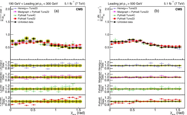
Figure 10 shows the corrected normalized differential distribution as a function of the cosine of the Nachtmann–Reiter angle in the inclusive four-jet sample. Most of the models follow the broad features of the data. However, the degree of agreement with data is different among

models. MADGRAPH+PYTHIA6 provides the best description of the data; HERWIG++ with

an-gular ordering in the parton shower is close to the data (the agreement is better than 5%), while

PYTHIA6 has the largest deviation (the agreement is typically between 10–12%).

9.2 Effect of hadronization, underlying event, and PDFs

The disagreement between data and the MC models may arise from the implementation of nonperturbative components in the simulation due to the fragmentation model or the choice of PDF set. These effects have been investigated by studying the uncertainties due to hadroni-zation model and PDF parametrihadroni-zation.

The MC models have different ways of modeling the underlying events and hadronization of the partons into hadrons. This may result in different predictions of the distributions of multijet variables depending on whether they are computed at the hadron or at the parton level. This

effect has been investigated by studying two different MC models: PYTHIA6 andHERWIG++.

This is done by evaluating the distributions at the parton and hadron level. PYTHIA6 uses

(17)

15 0 0.1 0.2 0.3 0.4 0.5 0.6 0.7 0.8 0.9 1 NR θ dcos dN . N 1 0.5 1.0 1.5 2.0 2.5 Herwig++ Tune23 Madgraph + Pythia6 TuneZ2 Pythia8 Tune4C Pythia6 TuneZ2 Unfolded data CMS NR θ cos 0 0.2 0.4 0.6 0.8 1 Data Pythia6 0.8 1.0 1.2 NR θ cos 0 0.1 0.2 0.3 0.4 0.5 0.6 0.7 0.8 0.9 1 Data Pythia8 0.81.0 1.2 NR θ cos 0 0.1 0.2 0.3 0.4 0.5 0.6 0.7 0.8 0.9 1 Data Madgraph 0.8 1.0 1.2 NR θ cos 0 0.1 0.2 0.3 0.4 0.5 0.6 0.7 0.8 0.9 1 Data Herwig++ 0.8 1.0 1.2 (7 TeV) -1 5.1 fb < 300 GeV T

(a) 0 0.1 0.2 0.3 0.4 0.5 0.6 0.7 0.8 0.9 1 NR θ dcos dN . N 1 0.5 1.0 1.5 2.0 2.5 Herwig++ Tune23 Madgraph + Pythia6 TuneZ2 Pythia8 Tune4C Pythia6 TuneZ2 Unfolded data CMS NR θ cos 0 0.2 0.4 0.6 0.8 1 Data Pythia6 0.8 1.0 1.2 NR θ cos 0 0.1 0.2 0.3 0.4 0.5 0.6 0.7 0.8 0.9 1 Data Pythia8 0.81.0 1.2 NR θ cos 0 0.1 0.2 0.3 0.4 0.5 0.6 0.7 0.8 0.9 1 Data Madgraph 0.8 1.0 1.2 NR θ cos 0 0.1 0.2 0.3 0.4 0.5 0.6 0.7 0.8 0.9 1 Data Herwig++ 0.8 1.0 1.2 (7 TeV) -1 5.1 fb > 500 GeV T Leading jet p (b)

Figure 10: Corrected normalized distribution of the cosine of the Nachtmann–Reiter angle. The other explanations are the same as Fig. 5.

are done differently in the two models. A generator-level study is carried out for both these models, where the effect of hadronization is studied using distributions from jets at parton-and hadron-level. The ratio of the parton- to the hadron-level distribution is then compared. The mean difference between the two hadronization models is typically less than 5%.

Comparisons are also made to different tunes of the underlying event models withinPYTHIA6.

The tunes (D6T, DW, P0, Z1, Z2, Z2*) [10, 11, 38–40] differ in the cutoff used to regularize the

1/p4_Tdivergence for final-state partons, the ordering of the showers (virtuality ordering vs. pT

ordering), multiparton interaction model, PDFs, and data sets used in the tune. The resulting distributions agree typically within 5%, so the disagreements with the data cannot be fully explained by this effect.

The MC models use CTEQ6 as the default PDF parametrization. There are many different PDF sets, which are based on different input data, assumptions, and parametrizations. Thus any calculation of a cross section or distributions in the simulation depends on the choice of PDF set. Also, each PDF set has its own errors from its parametric assumptions and data input to fitting. The effect of the PDF set choice on the multijet variables is calculated according to the recommendation of PDF4LHC group [41, 42]. Since comparisons are made only with leading order Monte Carlo models in this paper, only two leading order PDF sets are used in this comparison: CTEQ6l and MSTW2008lo68cl [43]. The uncertainties are found to be typically at

the level of 1.0–2.0% depending on the variable type and pTrange considered.

10 Summary

Distributions of topological variables for inclusive three- and four-jet events in pp collisions measured with the CMS detector at a centre-of-mass energy of 7 TeV were presented using a

(18)

cor-16 10 Summary

rected for detector effects, and systematic uncertainties were estimated. These corrected

dis-tributions were compared with the predictions from four LO MC models: PYTHIA6,PYTHIA8,

HERWIG++, and MADGRAPH+PYTHIA6.

Distributions of three- and four-jet invariant mass from all models show significant deviation from the data at high mass. The fact that all models have a common PDF suggests that the PDF errors at high mass are underestimated. The PDFs at high invariant mass have recently been

constrained by CMS using dijet pT distributions[44].

The MADGRAPH simulations are based on tree-level calculations for two-, three-, and

four-parton final states, while PYTHIAandHERWIG++ can have only two partons in the final state

before showering. Not surprisingly, the three-jet predictions of MADGRAPH+PYTHIA6 give a

more consistent description of the distributions studied in this analysis. The notable exception

is at high x4(the next-to-leading jet), where two jets carry most of the CM energy. The difference

is probably due to a double counting of three-parton with two-parton (with a parton from showering) final states.

ThePYTHIAandHERWIG++ models give poor descriptions of the energy fractions in the

three-jet final state. In particular, the distributions of x3(the leading jet) show large shape differences

between data and theory that are inconsistent with PDFs or hadronization model

uncertain-ties. Since the distributions from MADGRAPH+PYTHIA6 agree with those from the data, the

discrepancies with PYTHIAand HERWIG++ are likely due to missing higher multiplicity ME,

which are present in MADGRAPH.

All the models compared in this study do remarkably well describing the four-jet Bengtsson–

Zerwas angle. ThePYTHIAmodels have some systematic deviation from the data in describing

the Nachtmann–Reiter angle. Parton showers with angular ordering, as implemented inHER

-WIG++, yield a better agreement with the measured data for these angular variables.

Acknowledgments

We congratulate our colleagues in the CERN accelerator departments for the excellent perfor-mance of the LHC and thank the technical and administrative staffs at CERN and at other CMS institutes for their contributions to the success of the CMS effort. In addition, we grate-fully acknowledge the computing centres and personnel of the Worldwide LHC Computing Grid for delivering so effectively the computing infrastructure essential to our analyses. Fi-nally, we acknowledge the enduring support for the construction and operation of the LHC and the CMS detector provided by the following funding agencies: the Austrian Federal Min-istry of Science, Research and Economy and the Austrian Science Fund; the Belgian Fonds de la Recherche Scientifique, and Fonds voor Wetenschappelijk Onderzoek; the Brazilian Fund-ing Agencies (CNPq, CAPES, FAPERJ, and FAPESP); the Bulgarian Ministry of Education and Science; CERN; the Chinese Academy of Sciences, Ministry of Science and Technology, and Na-tional Natural Science Foundation of China; the Colombian Funding Agency (COLCIENCIAS); the Croatian Ministry of Science, Education and Sport, and the Croatian Science Foundation; the Research Promotion Foundation, Cyprus; the Ministry of Education and Research, Esto-nian Research Council via IUT23-4 and IUT23-6 and European Regional Development Fund, Estonia; the Academy of Finland, Finnish Ministry of Education and Culture, and Helsinki Institute of Physics; the Institut National de Physique Nucléaire et de Physique des Partic-ules / CNRS, and Commissariat à l’ Énergie Atomique et aux Énergies Alternatives / CEA, France; the Bundesministerium f ür Bildung und Forschung, Deutsche Forschungsgemeinschaft, and Helmholtz-Gemeinschaft Deutscher Forschungszentren, Germany; the General Secretariat

(19)

References 17

for Research and Technology, Greece; the National Scientific Research Foundation, and Na-tional Innovation Office, Hungary; the Department of Atomic Energy and the Department of Science and Technology, India; the Institute for Studies in Theoretical Physics and Mathe-matics, Iran; the Science Foundation, Ireland; the Istituto Nazionale di Fisica Nucleare, Italy; the Ministry of Science, ICT and Future Planning, and National Research Foundation (NRF), Republic of Korea; the Lithuanian Academy of Sciences; the Ministry of Education, and Uni-versity of Malaya (Malaysia); the Mexican Funding Agencies (CINVESTAV, CONACYT, SEP, and UASLP-FAI); the Ministry of Business, Innovation and Employment, New Zealand; the Pakistan Atomic Energy Commission; the Ministry of Science and Higher Education and the National Science Centre, Poland; the Fundação para a Ciência e a Tecnologia, Portugal; JINR, Dubna; the Ministry of Education and Science of the Russian Federation, the Federal Agency of Atomic Energy of the Russian Federation, Russian Academy of Sciences, and the Russian Foun-dation for Basic Research; the Ministry of Education, Science and Technological Development of Serbia; the Secretar´ıa de Estado de Investigaci ón, Desarrollo e Innovaci ón and Programa Consolider-Ingenio 2010, Spain; the Swiss Funding Agencies (ETH Board, ETH Zurich, PSI, SNF, UniZH, Canton Zurich, and SER); the Ministry of Science and Technology, Taipei; the Thailand Center of Excellence in Physics, the Institute for the Promotion of Teaching Science and Technology of Thailand, Special Task Force for Activating Research and the National Sci-ence and Technology Development Agency of Thailand; the Scientific and Technical Research Council of Turkey, and Turkish Atomic Energy Authority; the National Academy of Sciences of Ukraine, and State Fund for Fundamental Researches, Ukraine; the Science and Technology Facilities Council, UK; the US Department of Energy, and the US National Science Foundation. Individuals have received support from the Marie-Curie programme and the European Re-search Council and EPLANET (European Union); the Leventis Foundation; the A. P. Sloan Foundation; the Alexander von Humboldt Foundation; the Belgian Federal Science Policy Of-fice; the Fonds pour la Formation à la Recherche dans l’Industrie et dans l’Agriculture (FRIA-Belgium); the Agentschap voor Innovatie door Wetenschap en Technologie (IWT-(FRIA-Belgium); the Ministry of Education, Youth and Sports (MEYS) of the Czech Republic; the Council of Sci-ence and Industrial Research, India; the HOMING PLUS programme of Foundation for Polish Science, cofinanced from European Union, Regional Development Fund; the Compagnia di San Paolo (Torino); the Consorzio per la Fisica (Trieste); MIUR project 20108T4XTM (Italy); the Thalis and Aristeia programmes cofinanced by EU-ESF and the Greek NSRF; and the National Priorities Research Program by Qatar National Research Fund.

References

[1] L3 Collaboration, “A test of QCD based on 3-jet events from Z0decays”, Phys. Lett. B 263

(1991) 551, doi:10.1016/0370-2693(91)90504-J.

[2] L3 Collaboration, “A test of QCD based on 4-jet events from Z0_{decays”, Phys. Lett. B 248}

(1990) 227, doi:10.1016/0370-2693(90)90043-6.

[3] D0 Collaboration, “Studies of topological distributions of inclusive three- and four-jet

events in pp collisions at√s =1800 GeV with the D0 detector”, Phys. Rev. D 53 (1996)

6000, doi:10.1103/PhysRevD.53.6000.

[4] CDF Collaboration, “Further properties of high-mass multijet events at the Fermilab proton-antiproton collider”, Phys. Rev. D 54 (1996) 4221,

(20)

18 References

[5] CMS Collaboration, “The CMS experiment at the CERN LHC”, JINST 3 (2008) S08004, doi:10.1088/1748-0221/3/08/S08004.

[6] T. Sj ¨ostrand, S. Mrenna, and P. Skands, “PYTHIA 6.4 physics and manual”, JHEP 05 (2006) 026, doi:10.1088/1126-6708/2006/05/026, arXiv:hep-ph/0603175. [7] G. Marchesini and B. R. Webber, “Monte Carlo simulation of general hard processes with

coherent QCD radiation”, Nucl. Phys. B 310 (1988) 461,

doi:10.1016/0550-3213(88)90089-2.

[8] I. G. Knowles, “Spin correlations in parton-parton scattering”, Nucl. Phys. B 310 (1988) 571, doi:10.1016/0550-3213(88)90092-2.

[9] I. G. Knowles, “A linear algorithm for calculating spin correlations in hadronic collisions”, Comput. Phys. Commun. 58 (1990) 271,

doi:10.1016/0010-4655(90)90063-7.

[10] R. Field, “Min-Bias and the Underlying Event at the LHC”, (2012). arXiv:1202.0901. [11] R. Field, “Early LHC Underlying Event Data - Findings and Surprises”, (2010).

arXiv:1010.3558.

[12] J. Pumplin et al., “New generation of parton distributions with uncertainties from global QCD analysis”, JHEP 07 (2002) 012, doi:10.1088/1126-6708/2002/07/012, arXiv:hep-ph/0201195.

[13] B. Andersson, G. Gustafson, G. Ingelman, and T. Sj ¨ostrand, “Parton fragmentation and string dynamics”, Phys. Rept. 97 (1983) 31, doi:10.1016/0370-1573(83)90080-7. [14] T. Sj ¨ostrand, “The merging of jets”, Phys. Lett. B 142 (1984) 420,

doi:10.1016/0370-2693(84)91354-6.

[15] T. Sj ¨ostrand, S. Mrenna, and P. Z. Skands, “A brief introduction to PYTHIA 8.1”, Comp. Phys. Comm. 178 (2008) 852, doi:10.1016/j.cpc.2008.01.036.

[16] R. Corke and T. Sj ¨ostrand, “Interleaved parton showers and tuning prospects”, JHEP 03 (2011) 032, doi:10.1007/JHEP03(2011)032.

[17] M. B¨ahr et al., “Herwig++ physics and manual”, Eur. Phys. J. C 58 (2008) 639,

doi:10.1140/epjc/s10052-008-0798-9, arXiv:0803.0883.

[18] M. B¨ahr, S. Gieseke, and M. H. Seymour, “Simulation of multiple partonic interactions in Herwig++”, JHEP 07 (2008) 76, doi:10.1088/1126-6708/2008/07/076.

[19] S. Gieseke, P. Stephens, and B. R. Webber, “New formalism for QCD parton showers”, JHEP 12 (2003) 045, doi:10.1088/1126-6708/2003/12/045,

arXiv:hep-ph/0310083.

[20] B. R. Webber, “A QCD model for jet fragmentation including soft gluon interference”, Nucl. Phys. B 238 (1983) 492, doi:10.1016/0550-3213(84)90333-X.

[21] J. Alwall et al., “MadGraph 5: going beyond”, JHEP 06 (2011) 128,

(21)

References 19

[22] S. Mrenna and P. Richardson, “Matching matrix elements and parton showers with HERWIG and PYTHIA”, JHEP 05 (2003) 040,

doi:10.1088/1126-6708/2004/05/040.

[23] GEANT4 Collaboration, “GEANT4—a simulation toolkit”, Nucl. Instrum. Meth. A 506 (2003) 250, doi:10.1016/S0168-9002(03)01368-8.

[24] M. Bengtsson and P. M. Zerwas, “Four-jet events in e+e−annihilation: Testing the

three-gluon vertex”, Phys. Lett. B 208 (1988) 306,

doi:10.1016/0370-2693(88)90435-2.

[25] O. Nachtmann and A. Reiter, “A test for the gluon selfcoupling in the reactions e+e−→4

jets and Z→ 4 jets”, Z. Phys. C 16 (1982) 45, doi:10.1007/BF01573746.

[26] CMS Collaboration, “Particle–Flow Event Reconstruction in CMS and Performance for

Jets, Taus, and Emiss_T ”, CMS Physics Analysis Summary CMS-PAS-PFT-09-001, 2009.

[27] CMS Collaboration, “Commissioning of the Particle-flow Event Reconstruction with the first LHC collisions recorded in the CMS detector”, CMS Physics Analysis Summary CMS-PAS-PFT-10-001, 2010.

[28] M. Cacciari, G. P. Salam, and G. Soyez, “The anti-ktjet clustering algorithm”, JHEP 04

(2008) 63, doi:10.1088/1126-6708/2008/04/063.

[29] M. Cacciari, G. P. Salam, and G. Soyez, “FastJet user manual”, Eur. Phys. J. C 72 (2012) 1896, doi:10.1140/epjc/s10052-012-1896-2, arXiv:1111.6097.

[30] CMS Collaboration, “Determination of jet energy calibration and transverse momentum resolution in CMS”, J. Instrum. 6 (2011) P11002,

doi:10.1088/1748-0221/6/11/P11002.

[31] CMS Collaboration, “Tracking and Primary Vertex Results in First 7 TeV Collisions”, CMS Physics Analysis Summary CMS-PAS-TRK-10-005, 2010.

[32] CMS Collaboration, “Identification and filtering of uncharacteristic noise in the CMS hadron calorimeter”, J. Instrum. 5 (2009) T03014,

doi:10.1088/1748-0221/5/03/T03014.

[33] T. Adye, “Unfolding algorithms and tests using RooUnfold”, in Proceedings of the PHYSTAT 2011 Workshop on Statistical Issues Related to Discovery Claims in Search Experiments and Unfolding, H. B. Prosper and L. L., eds., p. 313. CERN, Geneva, Switzerland, January, 2011. doi:10.5170/CERN-2011-006.313.

[34] G. D’Agostini, “A multidimensional unfolding method based on Bayes’ theorem”, Nucl. Instrum. Meth. A 362 (1995) 487, doi:10.1016/0168-9002(95)00274-X.

[35] A. Hocker and V. Kartvelishvili, “SVD approach to data unfolding”, Nucl. Instrum. Meth. A 372 (1996) 469, doi:10.1016/0168-9002(95)01478-0.

[36] CMS Collaboration, “Jet Energy Resolution in CMS at√s=7 TeV”, CMS Physics

Analysis Summary CMS-PAS-JME-10-014, 2011.

[37] CMS Collaboration, “Jet Performance in pp Collisions at√s=7 TeV”, CMS Physics

(22)

20 References

[38] R. Field, “Physics at the Tevatron”, Acta Physica Polonica B 39 (2008) 2611.

[39] P. Z. Skands, “The Perugia Tunes”, in Multiple partonic interactions at the LHC. Proceedings of the First International Workshop, MPI08, P. Bartalini and L. Fano, eds., p. 284. Perugia, Italy, 2009. arXiv:0905.3418.

[40] CMS Collaboration, “Study of the underlying event at forward rapidity in pp collisions

at√s=0.9, 2.76, and 7 TeV”, J. High Energy Phys. 04 (2013) 072,

doi:10.1007/JHEP04(2013)072.

[41] S. Alekhin et al., “The PDF4LHC Working Group Interim Report”, (2011). arXiv:1101.0536.

[42] M. Botje et al., “The PDF4LHC Working Group Interim Recommendations”, (2011). arXiv:1101.0538.

[43] A. D. Martin, W. J. Stirling, R. S. Thorne, and G. Watt, “Parton distributions for the LHC”, Eur. Phys. J. C 63 (2009) 189, doi:10.1140/epjc/s10052-009-1072-5,

arXiv:0901.0002.

[44] CMS Collaboration, “PDF constraints and extraction of the strong coupling constant from the inclusive jet cross section at 7 TeV”, CMS Physics Analysis Summary

(23)

21

A

The CMS Collaboration

Yerevan Physics Institute, Yerevan, Armenia V. Khachatryan, A.M. Sirunyan, A. Tumasyan

Institut f ¨ur Hochenergiephysik der OeAW, Wien, Austria

W. Adam, T. Bergauer, M. Dragicevic, J. Er ¨o, M. Friedl, R. Fr ¨uhwirth1, V.M. Ghete, C. Hartl,

N. H örmann, J. Hrubec, M. Jeitler1, W. Kiesenhofer, V. Kn ünz, M. Krammer1, I. Krätschmer,

D. Liko, I. Mikulec, D. Rabady2_{, B. Rahbaran, H. Rohringer, R. Sch ¨ofbeck, J. Strauss,}

W. Treberer-Treberspurg, W. Waltenberger, C.-E. Wulz1

National Centre for Particle and High Energy Physics, Minsk, Belarus V. Mossolov, N. Shumeiko, J. Suarez Gonzalez

Universiteit Antwerpen, Antwerpen, Belgium

S. Alderweireldt, S. Bansal, T. Cornelis, E.A. De Wolf, X. Janssen, A. Knutsson, J. Lauwers, S. Luyckx, S. Ochesanu, R. Rougny, M. Van De Klundert, H. Van Haevermaet, P. Van Mechelen, N. Van Remortel, A. Van Spilbeeck

Vrije Universiteit Brussel, Brussel, Belgium

F. Blekman, S. Blyweert, J. D’Hondt, N. Daci, N. Heracleous, J. Keaveney, S. Lowette, M. Maes, A. Olbrechts, Q. Python, D. Strom, S. Tavernier, W. Van Doninck, P. Van Mulders, G.P. Van Onsem, I. Villella

Universit´e Libre de Bruxelles, Bruxelles, Belgium

C. Caillol, B. Clerbaux, G. De Lentdecker, D. Dobur, L. Favart, A.P.R. Gay, A. Grebenyuk,

A. L´eonard, A. Mohammadi, L. Perni`e2, A. Randle-conde, T. Reis, T. Seva, L. Thomas, C. Vander

Velde, P. Vanlaer, J. Wang, F. Zenoni Ghent University, Ghent, Belgium

V. Adler, K. Beernaert, L. Benucci, A. Cimmino, S. Costantini, S. Crucy, S. Dildick, A. Fagot, G. Garcia, J. Mccartin, A.A. Ocampo Rios, D. Ryckbosch, S. Salva Diblen, M. Sigamani, N. Strobbe, F. Thyssen, M. Tytgat, E. Yazgan, N. Zaganidis

Universit´e Catholique de Louvain, Louvain-la-Neuve, Belgium

S. Basegmez, C. Beluffi3, G. Bruno, R. Castello, A. Caudron, L. Ceard, G.G. Da Silveira,

C. Delaere, T. du Pree, D. Favart, L. Forthomme, A. Giammanco4, J. Hollar, A. Jafari, P. Jez,

M. Komm, V. Lemaitre, C. Nuttens, D. Pagano, L. Perrini, A. Pin, K. Piotrzkowski, A. Popov5,

L. Quertenmont, M. Selvaggi, M. Vidal Marono, J.M. Vizan Garcia Universit´e de Mons, Mons, Belgium

N. Beliy, T. Caebergs, E. Daubie, G.H. Hammad

Centro Brasileiro de Pesquisas Fisicas, Rio de Janeiro, Brazil

W.L. Ald´a J ´unior, G.A. Alves, L. Brito, M. Correa Martins Junior, T. Dos Reis Martins, C. Mora Herrera, M.E. Pol, P. Rebello Teles

Universidade do Estado do Rio de Janeiro, Rio de Janeiro, Brazil

W. Carvalho, J. Chinellato6, A. Cust ´odio, E.M. Da Costa, D. De Jesus Damiao, C. De Oliveira

Martins, S. Fonseca De Souza, H. Malbouisson, D. Matos Figueiredo, L. Mundim, H. Nogima,

W.L. Prado Da Silva, J. Santaolalla, A. Santoro, A. Sznajder, E.J. Tonelli Manganote6, A. Vilela

(24)

22 A The CMS Collaboration

Universidade Estadual Paulistaa, Universidade Federal do ABCb, S˜ao Paulo, Brazil

C.A. Bernardesb, S. Dograa, T.R. Fernandez Perez Tomeia, E.M. Gregoresb, P.G. Mercadanteb,

S.F. Novaesa, Sandra S. Padulaa

Institute for Nuclear Research and Nuclear Energy, Sofia, Bulgaria

A. Aleksandrov, V. Genchev2, R. Hadjiiska, P. Iaydjiev, A. Marinov, S. Piperov, M. Rodozov,

G. Sultanov, M. Vutova

University of Sofia, Sofia, Bulgaria

A. Dimitrov, I. Glushkov, L. Litov, B. Pavlov, P. Petkov Institute of High Energy Physics, Beijing, China

J.G. Bian, G.M. Chen, H.S. Chen, M. Chen, T. Cheng, R. Du, C.H. Jiang, R. Plestina7, F. Romeo,

J. Tao, Z. Wang

State Key Laboratory of Nuclear Physics and Technology, Peking University, Beijing, China C. Asawatangtrakuldee, Y. Ban, Q. Li, S. Liu, Y. Mao, S.J. Qian, D. Wang, Z. Xu, W. Zou

Universidad de Los Andes, Bogota, Colombia

C. Avila, A. Cabrera, L.F. Chaparro Sierra, C. Florez, J.P. Gomez, B. Gomez Moreno, J.C. Sanabria

University of Split, Faculty of Electrical Engineering, Mechanical Engineering and Naval Architecture, Split, Croatia

N. Godinovic, D. Lelas, D. Polic, I. Puljak

University of Split, Faculty of Science, Split, Croatia Z. Antunovic, M. Kovac

Institute Rudjer Boskovic, Zagreb, Croatia

V. Brigljevic, K. Kadija, J. Luetic, D. Mekterovic, L. Sudic University of Cyprus, Nicosia, Cyprus

A. Attikis, G. Mavromanolakis, J. Mousa, C. Nicolaou, F. Ptochos, P.A. Razis Charles University, Prague, Czech Republic

M. Bodlak, M. Finger, M. Finger Jr.8

Academy of Scientific Research and Technology of the Arab Republic of Egypt, Egyptian Network of High Energy Physics, Cairo, Egypt

Y. Assran9_{, A. Ellithi Kamel}10_{, M.A. Mahmoud}11_{, A. Radi}12,13

National Institute of Chemical Physics and Biophysics, Tallinn, Estonia M. Kadastik, M. Murumaa, M. Raidal, A. Tiko

Department of Physics, University of Helsinki, Helsinki, Finland P. Eerola, G. Fedi, M. Voutilainen

Helsinki Institute of Physics, Helsinki, Finland

J. Härk önen, V. Karimäki, R. Kinnunen, M.J. Kortelainen, T. Lampén, K. Lassila-Perini, S. Lehti, T. Lindén, P. Luukka, T. Mäenpää, T. Peltola, E. Tuominen, J. Tuominiemi, E. Tuovinen, L. Wendland

Lappeenranta University of Technology, Lappeenranta, Finland J. Talvitie, T. Tuuva

(25)

23

DSM/IRFU, CEA/Saclay, Gif-sur-Yvette, France

M. Besancon, F. Couderc, M. Dejardin, D. Denegri, B. Fabbro, J.L. Faure, C. Favaro, F. Ferri, S. Ganjour, A. Givernaud, P. Gras, G. Hamel de Monchenault, P. Jarry, E. Locci, J. Malcles, J. Rander, A. Rosowsky, M. Titov

Laboratoire Leprince-Ringuet, Ecole Polytechnique, IN2P3-CNRS, Palaiseau, France

S. Baffioni, F. Beaudette, P. Busson, C. Charlot, T. Dahms, M. Dalchenko, L. Dobrzynski, N. Filipovic, A. Florent, R. Granier de Cassagnac, L. Mastrolorenzo, P. Min´e, C. Mironov, I.N. Naranjo, M. Nguyen, C. Ochando, G. Ortona, P. Paganini, S. Regnard, R. Salerno, J.B. Sauvan, Y. Sirois, C. Veelken, Y. Yilmaz, A. Zabi

Institut Pluridisciplinaire Hubert Curien, Universit´e de Strasbourg, Universit´e de Haute Alsace Mulhouse, CNRS/IN2P3, Strasbourg, France

J.-L. Agram14, J. Andrea, A. Aubin, D. Bloch, J.-M. Brom, E.C. Chabert, C. Collard, E. Conte14,

J.-C. Fontaine14, D. Gel´e, U. Goerlach, C. Goetzmann, A.-C. Le Bihan, K. Skovpen, P. Van Hove

Centre de Calcul de l’Institut National de Physique Nucleaire et de Physique des Particules, CNRS/IN2P3, Villeurbanne, France

S. Gadrat

Université de Lyon, Université Claude Bernard Lyon 1, CNRS-IN2P3, Institut de Physique Nucléaire de Lyon, Villeurbanne, France

S. Beauceron, N. Beaupere, G. Boudoul2, E. Bouvier, S. Brochet, C.A. Carrillo Montoya,

J. Chasserat, R. Chierici, D. Contardo2, P. Depasse, H. El Mamouni, J. Fan, J. Fay, S. Gascon,

M. Gouzevitch, B. Ille, T. Kurca, M. Lethuillier, L. Mirabito, S. Perries, J.D. Ruiz Alvarez, D. Sabes, L. Sgandurra, V. Sordini, M. Vander Donckt, P. Verdier, S. Viret, H. Xiao

Institute of High Energy Physics and Informatization, Tbilisi State University, Tbilisi, Georgia

Z. Tsamalaidze8

RWTH Aachen University, I. Physikalisches Institut, Aachen, Germany

C. Autermann, S. Beranek, M. Bontenackels, M. Edelhoff, L. Feld, A. Heister, O. Hindrichs, K. Klein, A. Ostapchuk, F. Raupach, J. Sammet, S. Schael, J.F. Schulte, H. Weber, B. Wittmer,

V. Zhukov5

RWTH Aachen University, III. Physikalisches Institut A, Aachen, Germany

M. Ata, M. Brodski, E. Dietz-Laursonn, D. Duchardt, M. Erdmann, R. Fischer, A. G ¨uth, T. Hebbeker, C. Heidemann, K. Hoepfner, D. Klingebiel, S. Knutzen, P. Kreuzer, M. Merschmeyer, A. Meyer, P. Millet, M. Olschewski, K. Padeken, P. Papacz, H. Reithler, S.A. Schmitz, L. Sonnenschein, D. Teyssier, S. Th ¨uer, M. Weber

RWTH Aachen University, III. Physikalisches Institut B, Aachen, Germany

V. Cherepanov, Y. Erdogan, G. Fl ¨ugge, H. Geenen, M. Geisler, W. Haj Ahmad, F. Hoehle,

B. Kargoll, T. Kress, Y. Kuessel, A. K ¨unsken, J. Lingemann2, A. Nowack, I.M. Nugent, O. Pooth,

A. Stahl

Deutsches Elektronen-Synchrotron, Hamburg, Germany

M. Aldaya Martin, I. Asin, N. Bartosik, J. Behr, U. Behrens, A.J. Bell, A. Bethani, K. Borras, A. Burgmeier, A. Cakir, L. Calligaris, A. Campbell, S. Choudhury, F. Costanza, C. Diez Pardos, G. Dolinska, S. Dooling, T. Dorland, G. Eckerlin, D. Eckstein, T. Eichhorn, G. Flucke,

J. Garay Garcia, A. Geiser, P. Gunnellini, J. Hauk, M. Hempel15, H. Jung, A. Kalogeropoulos,

M. Kasemann, P. Katsas, J. Kieseler, C. Kleinwort, I. Korol, D. Kr ¨ucker, W. Lange, J. Leonard,