Capital structure and Business cycle

(1)

Capital structure and business cycle

Francisco Silva Ferreira

[email protected]

Dissertation for the Master in Management

Supervisors:

Prof. Miguel Sousa

Prof. Manuel Luís Costa

(2)

Biographical note

Francisco Ferreira was born in Porto, Portugal in September 12th, 1994. He

received his bachelor degree in Economics from Faculdade de Economia do Porto in 2015. In the same year he joined the Master in Management at the same university, in which he is currently studying.

(3)

Acknowledgements

This dissertation would not be possible without the help of some people that gave their contribution during this work.

First, I would like to thank my supervisors Profs. Miguel Sousa and Manuel Luis Costa for their support, availability and patience. Without their encouragement and guidance I couldn´t have accomplished this dissertation.

I am also, very grateful to Mr. António Silva at Bureau Van Dijk and Paula Carvalho at FEP’s library who were very helpful in obtaining the data needed for this dissertation, and made it possible for me to have a more complete study.

Finally, I want to thank my family and friends for their support, especially to Margarida Couto that was always there to motivate me and help me finishing this dissertation.

(4)

Abstract

This dissertation intends to study the impact of business cycle fluctuations in firms’ capital structure decisions. Since the seminal work of Modigliani and Miller (1958) on firms financing structures, many studies have been conducted and theories created in order to understand managers’ decisions. Still, there is a big debate on how firms decide their financing mix and what are the factors influencing these decisions. This study contributes to the deepening of knowledge on the factors affecting managers’ decisions and test empirically the theories on this subject. This work aims to study the relation between economic conditions and firms’ financing decisions. The understanding of this relation will help understand which factors influence managers’ decisions and contribute to more efficient decisions when deciding about financing issues. In order to carry out the empirical study we use a sample of non-listed industrial firms from euro area countries. The regressions conducted allow for the conclusion that leverage is counter-cyclical. Another interesting finding is that capital structure determinants impact leverage in different ways depending on the cycle phase. This finding leads us to conclude that larger firms tend to take advantage of better financing conditions while smaller firms are not able to benefit from these lower financing costs. These results confirm the predictions of the pecking order theory.

Key-words: Capital structure, Business cycle, Macroeconomic conditions, Small

(5)

Resumo

Esta dissertação tem como objectivo o estudo do impacto do ciclo económico na estrutura de capitais das empresas. Desde do estudo de Modigliani and Miller (1958) que muitos outros estudos sobre o financiamento de empresas foram desenvolvidos assim como várias teorias. Contudo, ainda existe um grande debate sobre a forma como os gestores decidem financiar a actividade das suas empresas e sobre quais os factores que influenciam essas mesmas decisões. Este estudo serve para aprofundar o conhecimento que existe nesta área de forma a tentar compreender melhor o que leva os gestores a escolher divida no lugar de capitais próprios ou vice-versa. Desta forma, é analisado o impacto das condições económicas na estrutura de capitais de modo a compreender o impacto dos diferentes factores neste tipo de decisões e assim contribuir para a melhoria destas. Para isto, usamos uma amostra composta por empresas da zona euro não cotadas em bolsa do sector industrial. Os resultados do estudo permitem concluir que a alavancagem é contra cíclica. Também concluímos que os diferentes determinantes de estrutura de capitais alteram a sua relevância consoante a fase do ciclo em que se encontram as empresas. A alteração do impacto dos diferentes factores leva-nos a concluir que as grandes empresas têm maior facilidade na obtenção de crédito enquanto as empresas mais pequenas tendencialmente terão mais dificuldade em se financiar. Estes resultados confirmam as previsões da teoria pecking order de estrutura de capitais.

Key-words: Capital structure, Business cycle, Macroeconomic conditions, Small

(6)

List of figures

Figure 1 - The static - tradeoff theory of capital structure ... 5 Figure 2 - Evolution of the Eurozone output gap ... 29

List of tables

Table 1 - Firms’ distribution by country ... 27 Table 2 - Sample summary statistics ... 28 Table 3 - Regressions with leverage as dependent variable ... 31

(9)

1. Introduction

Capital structure decisions have been in debate for a long time with many theories being developed and tested. Nevertheless, there is no consensus on which theory or theories describe better financing decisions of firms. Many empirical tests have been conducted and show that none of the theories describe completely firms’ financing decisions. This study aims to add knowledge on how firms’ financing decisions are affected by business cycle factors, contributing to a better understanding of firms’ financial structure.

This dissertation intends to answer the questions: How European industrial companies react to changes in business cycle? Which are the factors affecting capital structure decisions? How business cycles affect the impact of these factors on capital structure? In fact, all these answers are not yet answered in the literature for industrial companies. Moreover, the relation between capital structure and economic conditions is not a much studied topic, and there is a lack of industry studies, which is important because economic fluctuations may not affect all sectors the same way.

To achieve the goals proposed, we gathered data for non-listed industrial companies in Europe and studied the impacts of changes in the business cycle on their capital structure. This choice for non-listed firms comes from the fact that almost all of the previous studies use listed companies which may bias their sample since these firms are the ones that have more access to financial markets and tend to have more similar reactions. Also, the choice for just including industrial firms is justified by the fact that economic conditions affect the different sectors in different manners. The industrial sector is more exposed to international competition and thus it is expected that it reacts more to major changes in economic conditions, which makes this sector an interesting choice to be studied.

The results of this study suggest that firms present counter-cyclical leverage. We also find that the capital structure determinants change their impact depending on the phase of the business cycle.

These results are line with the conclusions of pecking order theory developed by Myers and Majluf (1984).

(10)

The result of this dissertation will help managers choose better and in a more informed way their firms’ financing. Also for researchers, this study will provide an empirical sample of industrial firms that can be useful for the development of new theories related to capital structure in specific sectors.

This report is structured as follows: In chapter 2. we make a review of the main

theories of capital structure, business cycle and the studies that merge the two topics. In chapter 3. we expose the methodology employed in this study and assess the sample used. Chapter 4. presents the main results of the study and chapter 5. the conclusions.

(11)

2. Literature Review

In this chapter we will make a literature review of what has been written about capital structure and business cycle. In section 2.1 and 2.2 we will present the definitions of capital structure and business cycle. In section 2.3 the main theories of capital structure will be assessed and compared. Section 2.4 describes the main capital structure determinants. Section 2.5 contains a review of the main business cycle theories and section 2.6 presents the main studies on capital structure and business cycle.

2.1. Capital structure definition

Before Modigliani and Miller (1958), economists assumed the decisions of financing mix as given. Theorists assumed that the cost of capital was a constant interest rate paid on bonds. To that interest rate they added a risk premium to control for market volatility and keep the cost of capital equal to a fixed rate. Modigliani and Miller theorem introduced the basis for the study of firms’ financing mix by trying to understand what makes firms finance their investments with debt or equity. Myers (2001) describes capital structure as follows: “The study of capital structure has the

purpose of explaining the mix of securities and other financing sources used by firms to finance real investment. (Myers 2001)

2.2. Business cycle definition

Business cycle refers to the fluctuations in the level of output, employment and inflation in a given economy. According to Black (1981), business cycles are the consequence of changes in both demand and supply conditions. These changes can be explained by many factors such as technology or even tastes. The concept of business cycle is defined by Gordon (2008) as the changes between periods of rapid and slow growth of GDP:

“Business cycles consist of expansions occurring at about the same time in many economic activities, followed by similarly general recessions and recoveries that merge into the expansion phase of the next cycle.” (Gordon, 2008)

2.3. Capital structure theories

The debate about capital structure and their influence on investment projects began after the seminar work of Modigliani and Miller in 1958. In this study, the authors

(12)

proved that under the conditions of perfect markets and no frictions the capital structure does not affect the value of the firm. It is irrelevant for the value of the firm with how much debt or equity it is financed.

Nevertheless, according to Myers (2001) the capital structure does impact firm value due to three main factors: taxes, asymmetric information and agency costs;

This view in which capital structure does have an impact in the value of the firm has been a topic of research with many economists suggesting different theories. Among the theories of optimal capital structure there are three that stand out: trade-off theory, picking order theory and cash-flow theory.

2.3.1. Trade-off theory

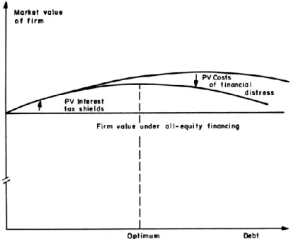
The trade-off theory is based on the fact that taxes can have an important role on the financing decisions firms make. The firms’ optimal capital structure is set by balancing the benefits of additional debt with its costs. In this case the benefits are measured by the tax shields provided by debt, and the costs to be taken into account are bankruptcy costs. Managers should combine both equity and debt in a way that maximizes the value of the firm. The main idea of this theory is well summed up by Myers:

“…the firm will borrow up to the point where the marginal value of tax shields on additional debt is just offset by the increase in the present value of possible costs of financial distress.” (Myers, 2001)

To easily understand trade-off theory, Figure 1 gives us a complete perspective of how firms should behave in the presence of different costs and benefits (Myers, 1984).

(13)

Figure 1 – The static - tradeoff theory of capital structure

The consequence of this theory, in general, is that firms will have moderate levels of debt since the weighting of benefits and costs will establish the limits to leverage. One of the criticisms to this view is that firms with low probability of financial distress would have the incentive to have high debt ratios, which is not a general pattern. Actually, this type of firms may have low debt ratios because they generate the necessary cash-flow to sustain their activity. The fact that firms don´t issue debt when the marginal benefits are higher than marginal costs reveals that interest tax shields may not have the relevance discussed in the literature. However, previous studies had shown empirically (see Wald 1999) that the relation between profitability and debt is inversely proportional, being the most important determinant of debt. This means that the trade-off theory does not fit with the empirical studies on capital structure (see Myers (2001)). Summing up, the trade-off theory is one of the most important theories on optimal capital structure and explains why certain firms have incentive to have a balanced capital structure with medium levels of debt. Nevertheless, this theory fails to explain that the most profitable firms don´t have high debt ratios.

(14)

2.3.2. Pecking order theory

The pecking order theory was first presented by Myers and Majluf (1984) The authors assumed that the firm would need external financing if it decides to pursue an investment opportunity. Besides that, managers are assumed to act in the best interest of shareholders (there are no agency costs) and managers have more information then external investors (there is information asymmetry).

In the case the firm issues new shares, the manager can either set an overvalued price or an undervalued price. In the latter, the manager is transferring wealth from old to new shareholders when in the case of an overvalued price the opposite happens. Myers and Majluf (1984), as mentioned before, assumed that there are no agency problems, thus the manager won´t issue new shares on an undervalued price. The new shares will be priced at an equal or higher level than their fair price. Anticipating the shares are overvalued, investors will cause a price drop in the market. The equity issues can be regarded as having informational value. The conclusion of this market reaction is that managers only will issue new shares if the costs of wealth transferring are offset by the benefits of the growth opportunity. According to the authors, usually the perception of investors tends to overvalue the costs and undervalue the benefits, leading managers to opt not to issue new stock because the new issues will reduce the firm’s value.

In the case of debt issue the market reaction does not have the same impact in the firm’s valuation. According to Myers (2001) the informational value of the issues plays a major role here since it reduces information asymmetries. The managers that are confident about the firm’s future performance will issue debt since they think that the firm will be able to repay it. The managers will decide for equity only if they are not able to increase their leverage (when debt has already high cost due to firm’s risk). Thus, the investors will react negatively to equity issues, reading them as sign of the inability of the company to increase its leverage.

The previous reasoning leads to the pecking order formulated by Myers and Majluf (1984) as presented in Myers (2001):

“1) Firms prefer internal to external finance. (Information asymmetries are assumed relevant only for external financing.)

2) Dividends are "sticky," so that dividend cuts are not used to finance capital expenditure, and so that changes in cash requirements are not soaked up in short-run

(15)

dividend changes. In other words, changes in net cash show up as changes in external financing.

3) If external funds are required for capital investment, firms will issue the safest security first, that is, debt before equity. If internally generated cash flow exceeds capital investment, the surplus is used to pay down debt rather than repurchasing and retiring equity. As the requirement for external financing increases, the firm will work down the pecking order, from safe to riskier debt, perhaps to convertible securities or preferred stock, and finally to equity as a last resort.

4) Each firm's debt ratio therefore reflects its cumulative requirement for external financing.” (Myers, 2001)

The major criticisms to this model are related to one of its assumptions. The assumption that managers act in the best interest of the shareholders is considered a strong one. Myers and Majluf (1984) don´t consider the rewards received by managers as a factor affecting the debt/equity mix. In fact, Ross (1977) studies the effect of manager’s compensation and finds a relation between the firm’s reward system and the capital structure choice.

The assumption of pecking order that managers act in the interest of the shareholders may be questioned according to Jensen and Meckling (1976); who put the agency costs problem in the center of capital structure debate.

2.3.3. Agency costs and firms financing mix

To explain the theories related with agency problems it is important to clarify this concept. According to Jensen and Meckling (1976), an agency relationship arises when a person or more act in the name of another one. The person acting in behalf of someone is called the agent and the represented person is called the principal. This is the type of relationship that exists in firms due to the separation between management and ownership. In the case of firms the principals can be either the shareholders or debtholders, while the agents are the managers. The agency problem arising in this case is that managers may have incentives to not behave in the best interests of shareholders or debtholders. To avoid this situation, the principal can take measures to ensure the agent behave in its best interest such as the design of a rewarding system that avoids misbehavior. Even in case the system would be totally effective (which never occurs),

(16)

the principal needs to incur in costs to monitor the agent. Jensen and Meckling (1976) define agency costs as the sum of three types of costs:

1. Monitoring expenditure by the principal 2. Bonding expenditures by the agent 3. Residual loss.

The first has to do with the cost of monitoring the agent’s behavior with rewards and penalties. It is related with the system used to encourage the agent to comply with the principal’s interests. The second is explained by Jensen and Meckling (1976) as the result of actions established by the principal to be carried out, in order to guarantee the agent uses the resources in the principal’s best interests. Finally, the third cost is the one related to the lack of efficiency of the monitoring system. In this case, the residual loss is the cost occurring when the system fails to ensure the agent behaves accordingly.

Because of separation between ownership and management, it is expected that there are agency costs due to the need to monitor the manager’s behaviour. This agency problem also exists between debtholders and shareholders. Since equity is a residual claim, in the case of bankruptcy, shareholders have interest in having the lower debt possible, for them to appropriate the maximum resources they can. There are three ways of shareholders to expropriate debtholders’ wealth by giving different incentives to their managers:

1. To invest in riskier projects; these investments will increase the rewards for shareholders but if the investment goes wrong, the debtholders are the ones bearing the cost.

2. To borrow money from investors and distribute dividends to shareholders; this will devalue debt and increase equity value.

3. To reduce the equity-financed investment; once again the risk will be transferred to creditors.

4. To conceal problems from creditors to buy time; this will virtually increase debt maturity and increase debt risk.

All these conflicts of interest between the different stakeholders in the firm will have consequences in the amount of debt and equity the firm will issue. This theory helped trade-off theory in giving a basis to justify the financial distress costs as an important cost when deciding the financing mix.

(17)

2.4. Determinants of capital structure

In order to assess the impact of economic conditions in firms financial structure, it is important to address the other factors that affect firm’s financing mix. Thus, in this section we will present the main determinants of capital structure according to the literature. There are many studies with the purpose of finding the determinants of capital structure with different conclusions regarding the impact of the different factors. In fact, Titman and Wessels (1988) conclude that the uniqueness of competencies or assets, industry, firm size and profitability do have an impact on capital structure choice. Also Öztekin (2015) studied the factors that affect the choice of capital structure worldwide and find that profits, firm size, tangibility, industry leverage and inflation do have an impact on firms’ financing mix. He also argues that institutional differences between countries have an impact on both the strength of the different factors and the speed of adjustment of capital structure to the optimal level. In this regard, Rajan and Zingales (1995) give their contribution by studying the impact of different institutional frameworks across G7 countries, advancing that taxes, bankruptcy laws, type of financial intermediation and corporate governance laws impact financing decisions.

2.4.1. Institutional factors

Previous studies from Rajan and Zingales (1995) and Öztekin (2015) find evidence that institutional environment have an impact on leverage. Öztekin (2015) argues that institutional framework can enhance the strength of the other factors such as firm sector, profitability and inflation. Öztekin (2015) also finds evidence that institutional environment have an impact on capital structure adjustment speed. If the laws of a certain country make it more costly to issue equity or debt, firms will take more time to adjust to the optimal level. For Öztekin (2015) the channels through which institutional framework impact capital structure are: bankruptcy laws, creditor protection laws, taxes, shareholder protection laws, accounting standards and information disclosure. Rajan and Zingales (1995) criticizes previous studies (see Borio (1990)) which conclude that the type of financial intermediation (bank oriented vs market oriented) is the main institutional factor affecting leverage. They argue instead, that the most relevant institutional factors are: tax code, bankruptcy laws, stage of development of bond markets and ownership patterns.

(18)

2.4.1.1. Taxes

According to Rajan and Zingales (1995), previous literature like Mayer (1990) concluded that taxes don´t impact the capital structure choices. However they contest this idea by arguing that Mayer’s study only uses corporate taxes and doesn´t capture the effect of personal taxes. In fact, they argue that studying the impact of taxes on capital structure is a difficult task since assumptions can completely change the conclusions. Rajan and Zingales (1995) using both corporate and personal taxes find that taxes do have an impact on leverage on an aggregate level but only considering the marginal tax rate for income of individuals. Öztekin (2015) also presents evidence that taxes and non-debt tax shields in countries with higher tax rates do have an impact on

leverage. On the other hand, Titman and Wessels (1988) don´t find evidence of the

impact of depreciation tax shield and investment fiscal credits on capital structure. Contrarily, DeAngelo and Masulis (1980) find that firms with higher depreciation and investment tax credits have higher leverage. Titman and Wessels (1988) acknowledge, however, that their conclusion can be related with the methodology used in the paper. To sum up, the most recent studies find evidence of the impact of taxes on leverage levels if considered high income personal taxes or countries with higher taxation rates.

2.4.1.2. Bankruptcy law

Bankruptcy code is one of the institutional factors that can have a direct impact on firms’ capital structure due to the incentives given to managers, creditors and shareholders. According to Rajan and Zingales (1995) bankruptcy laws have an important impact on the decisions from managers, shareholders or creditors. In fact, they mention three main aspects of bankruptcy code: the enforcement of creditor rights, the ability of creditors to sanction managers if firms get in financial distress and the cost of the bankruptcy process. They find that across the countries studied this type of laws have different focus, while ones are more firm protective, the others are more creditors protective. If the bankruptcy code is well designed it enforces the rights of both the creditors and the firm and, thus, reduces the time and cost of financial distress processes. Öztekin (2015) follows the conclusions in Rajan and Zingales (1995) and finds that bankruptcy laws influence the level of leverage. In fact, both papers find

(19)

evidence that in countries with more effective bankruptcy laws, firms have higher levels of debt since creditors take less time to recover their money, being more willing to lend.

2.4.1.3. Ownership and control

Rajan and Zingales (1995) advance the hypothesis that shareholders composition and control are relevant to define firms’ financing mix. However, they find dubious evidence on the effect of this factor. They argue that the existence of large shareholders should reduce agency costs and increase equity issues since large shareholders have more available resources. The opposite can happen if the shareholders are mainly banks that will have interest in lending money instead of giving it in the form of equity. Although they don´t find clear evidence for this factor, they think that ownership and control should have an impact on capital structure in that firms in more competitive control markets are more exposed to hostile takeovers, thus issuing more debt to protect themselves.

2.4.1.4. Shareholder protection laws

This institutional factor can have an important impact on capital structure since it can change the will of investors to finance firms with equity. Öztekin (2015) says that even though there is no consensus on this matter, strong shareholder protection laws should encourage equity financing since it reduces monitoring and contracting costs. This conclusion is based on previous literature on this subject (see Fan et al. (2012) and Acemoglu and Johnson (2005)) where weaker institutions lead to more debt financing.

2.4.2. Firm size

There is a consensus in the literature that firm size is relevant when it comes to define capital structure. Titman and Wessels (1988) and Öztekin (2015) find evidence of the impact of this factor on firms’ capital structures. Both studies find that larger firms tend to have more debt. Titman and Wessels (1988) justify this conclusion with the fact that bigger firms have lower costs when issuing securities and, thus, have more capacity to issue new debt.

(20)

2.4.3. Profitability

Profitability is also a factor that impacts firms’ financing mix. As Titman and Wessels (1988) argue, the impact of profitability on capital structure can be explained in the light of the pecking order theory. Actually, the capacity of generating profits and cash-flow impact financing decisions in the sense of pecking order theory: if a firm is more profitable, it will generate more internal funding and contract less debt. Also Öztekin (2015) find evidence internationally for the impact of profitability on firms’ financing.

2.4.4. Tangibility

Tangibility is an important factor that affects firms’ capital structure. Titman and Wessels (1988) and Öztekin (2015) find that tangibility do have an impact on firms’ financing patterns. They find that firms that possess more tangible assets tend to have more debt, the case being that they have more assets to give as collateral and thus creditors are more willing to lend them money.

2.4.5. Industry

The previous literature finds evidence of the impact of the firms’ sector on leverage levels. As a matter of fact, Titman and Wessels (1988) defend that firms in more specific sectors (or less diversified) have lower leverage due to higher liquidation costs. This is related with uniqueness of assets: industries that are more reliant on specific assets and knowledge will tend to have less debt. Lower debt levels reduce the probability of bankruptcy and thus, the probability of losing these valuable assets. Öztekin (2015) also finds that industry has an impact on capital structure arguing that firms in sectors with higher aggregate leverage tend to have more debt.

2.5. Business cycle theories

In order to study economic fluctuations it is important to understand how people behave economically. According to Black (1981) people seek for profit opportunities that maximize profitability and minimize risk. In fact, Black (1981) argues that people want three things when investing: high expected returns, low risk and high value.

Nevertheless, people usually don´t find all these characteristics in an asset or investment. As in every economic context there is a trade-off between these three

(21)

features. It is very difficult to find an investment that fulfils all these wants, so people will tend to opt by the one that maximizes their utility. People that are more risk averse will prefer an asset with lower expected returns and lower risk while the opposite will happen for people that are more risk takers.

As stated in the definitions, business cycles are fluctuations in economic conditions that affect almost every business sector. The business cycles can be captured by indicators such as the output, unemployment, inflation or even stock market prices. Economic conditions present fluctuations in output and employment, and not all the cycles have the same length or impact on the economy. Some cycles are stronger and more diffused while others are more rapidly overcome. However, it is expected that the output will follow a growth pattern over time despite the different business cycles occurred.

A main issue about business cycles in macroeconomic literature is to understand how fluctuations occur and study policies to reduce them. Until the 1930’s the general trend on macroeconomics was that markets adjust prices by the amount needed to match supply and demand. This trend was composed by the classical economists that assumed the prices were perfectly flexible. However, after the Great Depression, new theories were needed to explain why the markets didn´t reach the equilibrium. It was after 1929 that Keynes developed the Keynesian theory that assumed wages are rigid and do not adjust to equilibrium without intervention. This view also was criticized later when it failed to explain the oil crisis of the 1970’s that made prices rise while the economy was at recession. After the oil crisis the economists were split between two main views of business cycles, the new classics and the new Keynesians. Nevertheless, macroeconomics has three main views on business cycle:

 The new-classical;  The new-Keynesians;  Real business cycle.

2.5.1. The new classical macro

The new classical macro was at first developed by Milton Friedman and Edmund S. Phelps. They build up on the idea of continuous equilibrium in the labour and product markets and price adjustment. But they developed the hypothesis that

(22)

markets do not adjust perfectly, although individuals were acting optimally according to the price and wage levels. Friedman, Phelps and later Lucas argued that although individuals were acting according to their interests under a certain set of information, the information they were using could be incorrect. They assumed that households were unable to gather the correct information and that there was a problem of imperfect information. This problem was the root cause of business cycles since people weren´t deciding based on the true economic reality.

2.5.1.1. The “fooling” model

The fooling model or imperfect information model was first developed by

Milton Friedman (see Friedman (1968)) and then perfected by Phelps (see Edmund

(1967) and Phelps (1968)). Friedman defended that workers did not accurately predict the price level, opening the possibility for them to be “fooled” by firms. In other words, workers did not perceive correctly the prices while firms had the full price information, using this information advantage in their favour. This theory in practice would lead to an increase in profits of firms in the case of positive demand shock. The increase in profits will lead the economy to expansion until the workers perceive their estimates were wrong and ask for wage increase, reducing the firms’ profit. This last behaviour would lead to a recession. A similar model of imperfect information was also developed by Phelps but in his model both firms and workers did not perceive well the prices, generating economic fluctuations.

These models were subject to criticism mainly regarding the assumption of imperfect information. In the Friedman model, the criticisms were driven by the fact that there was no evidence of workers don´t have the correct information. Also, in the Phelps model, it is not probable that both firms and workers have imperfect information about prices since government and other institutions publish information on prices. The major criticism on this model is that it is very unlikely that firms and workers have incomplete information because they interact with other workers and firms in the market.

2.5.1.2. Rational expectations

This theory, developed by Lucas (see Lucas (1973)), also considers market

(23)

expectations. With this model, people would construct their expectations on the basis of imperfect information but they wouldn´t repeat the same mistake over and over again. From a statistic point of view, the forecasting errors should be random and independent from past mistakes. This model, like the previous one, argues that business cycles are created due to price changes that were not anticipated by workers and firms. The use of rational expectations in this model leads to a logical conclusion. If people decide correctly based on all available information, then anticipated changes in monetary policy won´t have any effect on real GDP. This lack of effectiveness of monetary policy is called the policy ineffectiveness proposition. This assumption created a huge impact on economists and policy makers since the only way to produce effects with monetary policy would be by creating price surprises.

Although the impact of this proposition was important in macroeconomics, some weaknesses were pointed out. Once again the problem was with the assumptions made

by Friedman and Phelps of imperfect information as the source of economic

fluctuations.

2.5.2. The new Keynesian macro

The new Keynesian macro derives from the Keynesian approach developed by Keynes after the Great Depression of 1929. Contrarily to the new classical models the new Keynesians do not assume that markets are always in equilibrium. Their models are created based on the assumption that prices do not adjust fast enough to balance supply and demand after a shock. In fact, Keynesians argue that markets deviate from equilibrium for long periods of time, creating an inadequate use of resources in the economy resources. This assumption is derived from the fact that firms and workers don´t want to reduce the number of hours of work or the production volume. These changes are the consequence of market imbalances that prevent market agents to produce and work the hours that maximize their welfare. The new Keynesians use the theory of rational expectations from Lucas and some microeconomic assumptions such as firms maximize profits and workers maximize utility. With the assumptions presented the new Keynesians show that the maximization of profits and utility on the micro level not always leads to social optimal at the aggregate level. The major criticism of this model is that it is very unlikely that firms and workers have imperfect information because they interact with other workers and firms in the market.

(24)

2.5.2.1. The new Keynesian model

In order to understand the model, it is important to clarify two aspects. First, the model has labour market and product market, where wages and prices are formed. The second is the distinction between nominal rigidity and real rigidity. According to Gordon (2008), “a nominal rigidity is a factor that inhibits the flexibility of the nominal

price level due to some factor, such as menu costs and staggered contracts.” while real

rigidity is “a factor that makes firms reluctant to change the real wage, the relative

wage, or the relative price”. (p. 567)

There are two explanations for the slow price adjustment. Nominal rigidity is explained by the existence of menu costs and long term contracts are barriers for price adjustment. On the other hand, real rigidity is originated by the stickiness of relative wages or relative prices. Although there are different price rigidities, these just serve to justify the price stickiness that prevents markets from clearing.

2.5.2.2. Nominal rigidities

There are several models that point out nominal rigidities as the source of economic fluctuations. First, the staggered price model points out the existence of contracts on goods prices and wages. This type of contracts establishes prices that are fixed for some time interval which sometimes is not adequate to current demand levels.

Second, another theory is menu costs, which consists in “any expense associated

with changing prices, including the costs of printing new menus or distributing new catalogues” (Gordon 2008). They explain the limitation in price movements, being a

probable cause of economic fluctuations since markets will be in an imbalance position if prices don´t adjust to the equilibrium level.

Third, according to the (S, s) pricing rule agents incur in a lump-sum cost every time prices are changed and, therefore, prices are only changed if the change in demand justifies the value paid to change prices. There is an interval of values in which economic agents do not change their prices.

The models presented in this section attempt to explain the existence of nominal price stickiness. The existence of price stickiness has an important consequence on the market, creating coordination failures. “Coordination failures occurs when there is no

(25)

society” Gordon (2008). The existence of coordination failures fits well in the

Keynesian view since the conclusion of the model is that it is necessary to intervene in the market in order to optimize micro level decisions and balance the economy on the aggregate level.

2.5.2.3. Real rigidities

As explained before, real rigidities exist when wages do not adjust relatively to prices or other wages. This type of price stickiness establishes the relation between the different prices.

According to Gordon (1990) there are several models that attempt to explain the sources of real rigidity on product market. One of these is the customer-search model from Okun et al. (1975) in which customers can pay a premium on the price of a certain product to avoid search costs. In other words, customers prefer to pay more for a product on their usual suppliers than to search to cheaper/better alternatives. The consequence of this model is that firms, in order to avoid losing their usual customers, won´t change prices as an answer to short run costs changes which may create price stickiness.

The previous model exposes an important point: the changes in marginal cost are independent from changes in aggregate demand. In fact this leads to a distinction between local and aggregate shocks and between demand and cost shocks. A model that takes into account this outcome from Okun et al. (1975) is the input-output table model. In this model each firm has a big set of suppliers and customers that can be affected by different shocks. Usually firms don´t know all their suppliers and it is very difficult to predict changes in the cost of their raw materials which creates an informational problem. The typical firm only changes their prices when the supplier communicates the price increase, creating inertia in the price adjustment. The firms avoid indexing their prices since cost changes depend on many factors that may be independent from aggregate demand. The reasoning of the input-output model leads to the understanding that there are coordination failures between economic agents. In the model, the source of these coordination failures is the asymmetric information available for each firm in the supply-chain. One can say that the main conclusion of this model is that the independence between cost and aggregate demand is the reason for the lack of price indexation.

(26)

The efficient wage model argues that higher wages will lead to increased productivity of labour. The relation between workers productivity and wages will increase competition in the labour market, which will make that firms will be reluctant to reduce their employees’ wages. This wage stickiness will prevent prices and wages from adjusting to the level that clear markets.

The new Keynesians have been criticized on the ground that the theory relies on a variety of explanations for their core assumption: price stickiness. The critics argue that the existence of long-term contracts may not be the source of price rigidity since business cycles occurred before the existence of organized unions.

2.5.3. Real business cycle

The real business cycle (RBC) can be considered an autonomous theory of the classical approach. Since the assumption of imperfect information of the fooling model presented before is not plausible, some classical economists developed the Real Business Cycle theory. This theory uses the basis of classical theories and assumes that prices adjust quickly to the equilibrium level. Thus, they assume that markets clear and that people behave accordingly to maximize their utility and firms to maximize their profit.

Contrarily to new Classical theories, they do not use the imperfect information assumption; instead they argue that business cycles are originated by real shocks. In other words, this means that changes in economic conditions are a consequence of supply shocks. As stated by Gordon (2008), these shocks can include new production

techniques, new products, bad weather, new sources of raw materials or price changes in raw materials. Following the classical tradition, the RBC model says that firms and

workers answer to these shocks maximizing their utility and firms their profits. There are no barriers to price formation and prices are perfectly flexible in this model. Thus workers can work the hours they want and firms establish the production volume in order to maximize profits.

This theory also faces some criticism regarding the realism of its assumptions. The critics argue that the real shocks advanced by RBC theory as the sources of economic fluctuations don´t occur as frequently or don´t have enough size to change the economic situation. This is the case for changes in technology that don´t have usually the size to

(27)

originate the impact observed on the economy. And, even though technology shocks usually have a significant impact in the economy, they are not as frequent as economic conditions change. Usually the changes in technology are small, providing little improvement; a big impact on the output from technology changes only occurs on the medium to long run.

2.6. Output Gap

In order to predict the reaction of firms’ capital structure to the business cycle it is important to include indicators that capture euro area economic conditions. Thus, we will use the output gap as a measure of the business cycle. The output gap is a synthetic measure of the economic cycle that measures the difference between the potential output and the actual GDP.

2.6.1. Potential growth

The output gap is one of the most important indicators to maintain a sustainable economic growth that is calculated based on the potential output. As described in Havik et al. (2014), the potential output:

“…constitutes a summary indicator of the economy's capacity to generate sustainable, non-inflationary, growth whilst the output gap is an indication of the degree of overheating or slack relative to this growth potential.” (p. 4)

In other words, the potential output is the measure of the economy growth capacity. The potential growth of an economy usually depends on the growth of labour and capital. However, an important part of economic growth comes from the way these two production factors are combined. The continuous optimization of technology is an important source of economic growth since an improved production function increases the productivity of labour and capital. The potential output growth will be the result of the evolution of labour, capital and technological development.

Since the potential output is not directly measurable, there are different methods to calculate it. The methods used can be either statistical or economic, but for the European case, the choice was the economic model for the following advantages: understand the factors behind potential output changes and understand the connection between policies and the outcomes of these policies. Also the possibility of changing assumptions according to economic conditions is an important feature since it gives the

(28)

model flexibility to be modelled depending on necessities. The authors of the model used for the European Union describe three characteristics that it has to have:

- Simplicity and ease of use;

- To fit all the European countries and be comparable between them;

- The estimates need to be accurate because it will be the base for budgetary monitoring among member states.

As mentioned before in the literature review on business cycles, two central objects of macroeconomics are the study of the business cycle and the growth potential of an economy. The output gap is, in fact, one of the most important indicators used by policy makers to analyse what policies to be implemented in order to reduce output cyclicality.

In the study we use both the output gap and a dummy variable that equals one when the output gap is positive (expansion) and zero when the output gap is negative (recession).

2.7. Capital structure and business cycle

In order to complete the study of previous literature it is important to present the main work on the relation between capital structure and business cycle. The studies on this topic have different approaches to explain the relation between the two concepts: some studies focus on the relation between economic conditions and credit spreads to explain changes in capital structure, others use a set of economic variables while others study the adjustment speed to the optimal capital structure level.

In the first group Chen (2010) and Hackbarth et al. (2006) reach different conclusions. The first argues that credit spreads are the consequence of firm risk which explains the lower leverage during recessions due to the increase in credit spreads. On the other hand, Hackbarth et al. (2006) find leverage counter-cyclical although they also agree on the impact of cash-flow and credit spreads to define firms’ capital structure.

In the group of studies that relate macroeconomic indicators with capital structure and firm determinants are Korajczyk and Levy (2003), Halling et al. (2016) and Levy and Hennessy (2007). Korajczyk and Levy (2003) divide their sample in constrained and unconstrained firms (respectively firms that are not able to pursue available investment opportunities and firms that are able to invest in these investment opportunities) and find that constrained firms have pro-cyclical leverage while

(29)

unconstrained firms have a counter-cyclical pattern for leverage. They advance the explanation that unconstrained firms are more able to time their issues and take advantage of market conditions while constrained firms are not. Halling et al. (2016) also divide their sample between constrained and unconstrained firms and although confirming counter-cyclical leverage for the majority of their sample, they do not find evidence of pro-cyclicality for the constrained sample. With a different approach, Levy and Hennessy (2007) study the behavior of leverage, equity and debt. They find that unconstrained firms have counter-cyclical leverage, counter-cyclical debt but pro-cyclical equity. On the other hand, they find that constrained firms have pro-pro-cyclical debt, pro-cyclical equity and do not find a consistent pattern for leverage.

Finally, Cook and Tang (2010) study the effect of macroeconomic conditions on capital structure adjustment speed. They find that firms respond faster to deviations in target leverage in expansions than in recessions.

After assessing all these studies on capital structure and business cycle, we conclude that there is space for deepening the research on this field. In fact there are not many studies that focus on the issue of macroeconomic conditions and capital structure. Although there is relative consensus on the conclusions of the existing studies, there are different samples that should be tested. For this study we choose European industrial companies that are not listed in stock exchanges. Our choice for this type of firm is easily justified by the fact that unlisted companies are the firms that more contribute to European economic growth and employment, thus being important to give some insights on their financing patterns and behaviors. Also we choose industrial companies because this type of firms compete more on a global scale, being more exposed to external competition, and operate in a more demanding environment. In order to be prepared to face international competition, it is important that European industrial firms have the best knowledge of their financial structure and are aware of the changes made by the majority of these firms when the business cycle changes. Nevertheless, the conclusions of this study are of great use for policy makers, namely the ones responsible for the monetary policy. Since this study focuses on firms from the euro area, this is a good opportunity for these policy makers to understand how firms react to changes in the economic environment and, thus, put in practice better measures to answer to these economic changes. The specificities of the euro area instructional framework can be an

(30)

important factor for these firms to decide their optimal capital structures. This dissertation aims to study how euro area firms react to changes in business cycle and may help understand whether firms in the monetary and economic union show different effects of the business cycle on firms capital structure. In fact, there are not many studies on this subject. As showed by Rajan and Zingales (1995) or Öztekin (2015) institutional factors have an impact on firms capital structure, which makes the study of euro area firms important to understand if these firms are affected differently due to euro zone peculiar framework. The fact that budget policies are decentralized decisions while monetary policy is centralized may affect firms financing differently than in the U.S. or other countries. For these reasons, our idea is that this study of the relationship between business cycle and capital structure in euro zone firms can add valuable insights on this topic.

(31)

3. Methodology

In this section we present the empirical setting employed in this study. First we present the regressions employed and the estimation method used. After this, we present the indicators that better describe capital structure changes, business cycle and firms’ specific factors and that will be used to complete the analysis. Finally, an analysis of the sample of firms and the data employed in this dissertation is carried out.

3.1. Empirical setting

The studies on this subject are conducted with different investigation methods. There are two main types of methodology employed in this type of studies: regression based studies or model based studies. The first consists in regressing different types of empirical data on variables that could affect capital structure decision and studies its real impact. The second, attempts to model both firm and economy behaviors and uses real data to simulate firm´s financing mix.

In this dissertation we use a regression based study since the main goal is to have an empirical approach to the topic of capital structure and not a theoretical one. To do so, we employ an empirical setting inspired on the ones used by Korajczyk and Levy (2003), Halling et al. (2016) and Cook and Tang (2010) which use firm specific factors and macroeconomic indicators as independent variables and leverage as dependent variables. In this study we conduct a few regressions in line with these studies, but we opt to follow more closely Rajan and Zingales (1995) in their study of the determinants of capital structure. To the regression from Rajan and Zingales (1995) we add an indicator of the business cycle obtaining the following regression:

(1)

𝐶𝑆_𝑡 = 𝛽 ∗ 𝐹𝑖𝑟𝑚_𝑡+ 𝛽 ∗ 𝑃𝑟𝑜𝑓_𝑡+ 𝛽 ∗ 𝑇𝑎𝑛𝑔_𝑡+ 𝛽 ∗ 𝑇𝑎𝑥_𝑡+ 𝛽 ∗ 𝑂𝐺_𝑡−1+ 𝜀_𝑡

where CS is a leverage indicator, Firm refers to firm size, Prof is a proxy for profitability, Tang is a tangibility indicator, Tax is an indicator that proxies for non-debt

(32)

Besides, we use a set of regressions that interact the business cycle with the different capital structure determinants to understand the indirect impact of the cycle on capital structure. The regressions have the following format:

(2)

𝐶𝑆_𝑡 = 𝛽 ∗ 𝐹𝑖𝑟𝑚_𝑡+ 𝛽 ∗ 𝑃𝑟𝑜𝑓_𝑡+ 𝛽 ∗ 𝑇𝑎𝑛𝑔_𝑡+ 𝛽 ∗ 𝑇𝑎𝑥_𝑡+ 𝛽 ∗ 𝑂𝐺_𝑡−1+ 𝛽 ∗ 𝑂𝐺_𝑡−1∗

𝐹𝑖𝑟𝑚_𝑡+ 𝛽 ∗ 𝑂𝐺_𝑡−1∗ 𝑃𝑟𝑜𝑓_𝑡+ 𝛽 ∗ 𝑂𝐺_𝑡−1∗ 𝑇𝑎𝑛𝑔_𝑡+ 𝛽 ∗ 𝑂𝐺_𝑡−1∗ 𝑇𝑎𝑥_𝑡+ 𝜀_𝑡

Where - as in equation (1) - CS is an indicator of leverage, Firm the indicator of firm size, Prof is the indicator for profitability, Tang is the indicator for tangibility, Tax is the indicator for tax shields, 𝑂𝐺𝑡−1 is the indicator for the business cycle in the previous

year, 𝑂𝐺_𝑡−1∗ 𝐹𝑖𝑟𝑚 is an interaction variable between business cycle and firm size,

𝑂𝐺_𝑡−1∗ 𝑃𝑟𝑜𝑓 is an interaction variable between business cycle and profitability,

𝑂𝐺𝑡−1∗ 𝑇𝑎𝑛𝑔 is an interaction variable between business cycle and tangibility, and

𝑂𝐺_𝑡−1∗ 𝑇𝑎𝑥 is an interaction variable between business cycle and non-debt tax shields.

3.1.1. Dependent variables

In this study we use two dependent variables. We study the impact of firm specific variables and macroeconomic conditions on leverage. Rajan and Zingales (1995) argue that the indicator used for leverage should vary with the purpose of the study. For their specific case they find that the most relevant indicator is the relation between debt and firms’ value. However, they use other indicators for leverage: the ratio between non-equity liabilities to total assets, the ratio of debt to total assets, the ratio of debt to net assets, debt to capital and the interest coverage ratio. In this study we use the following leverage measures: the ratio of total debt to total assets and the interest coverage ratio (EBIT/interest).

3.1.2. Macroeconomic variables

In order to measure the euro zone business cycle we use the output gap as macroeconomic variable. In fact, the output gap offers a synthetic measure of economic situation, making it easier to identify the changes of cycle. Also, this indicator is easily converted into index that can facilitate estimations. The output gap constitutes a good

(33)

proxy for the business cycle and gathers two important characteristics: it is simple to use and interpret and with just one indicator we can capture economic changes. Thus, in this study we use the output gap lagged one period and, alternatively, a dummy variable that assumes zero when there is a recession (negative output gap) and one when there is an expansion (positive output gap).

3.1.3. Firm specific variables

The firm specific variables are used in the regressions to control for the different characteristics of each firm. Titman and Wessels (1988) and Öztekin (2015) agree on four main firm specific determinants of capital structure. They find that firm size, profitability, taxes and tangibility are important determinants of capital structure. To control for the effect of these four factors we include a set of indicators in the regressions. For firm size we follow Halling et al. (2016) and Cook and Tang (2010) who use the logarithm of firm’s assets as proxy for this determinant. For profitability we will use the ratio of EBIT to Total assets. This ratio is also used by Cook and Tang (2010) and Halling et al. (2016). To control for tangibility we use the same measure as Cook and Tang (2010) and Halling et al. (2016) that employ the ratio of tangible assets to total assets. In order to account for non-debt tax shields we use the ratio of depreciation to total assets as Cook and Tang (2010).

There are other firm specific factors that are not included in this study such as firms’ industry since our sample is only composed by firms from the industrial sector. Contrary to the majority of studies (see Korajczyk and Levy (2003), Halling et al. (2016) and Cook and Tang (2010)) we do not use a measure of uniqueness since our data do not allow us to measure this factor.

3.1.4. Interaction variables

In equation (2) we use a set of interaction variables that show us how capital structure determinants impact leverage depending on the cycle. The use of these interaction terms will make it possible to observe the changes in the impact that the determinants have on capital structure depending on the business cycle. The coefficients of these variables allow us to understand the importance of these determinants during recessions and expansions.

(34)

3.2. Data collection and sampling

In this section we characterize the data used in this study and explain the criteria of selection of the firms from dataset. Also, we will assess statistically the type of firms that are included in the sample by studying their main financials and other relevant data. Our sample was selected from Amadeus database and includes all non-listed active firms from the euro area that operate in the industrial sector and don´t have a shareholder with more than 25% of equity (firms qualified as A+, A, A- in Amadeus’ independence indicator).

From the initial sample, we only kept the firms that have available financial information for the entire time frame (from 1996 to 2015) and have records for: fixed assets, total assets, shareholders’ funds, capital, non-current liabilities, long term debt, short term debt, net current assets, operating revenue and sales, EBIT, profit before and after taxes, net income and depreciation; this data must be available for at least half of the period of the study.

Data for business cycle, more specifically, the output gap for the euro zone was collected from AMECO database for the period between 1998 and 2015 and EconStats database from the International Monetary Fund for 1996 and 1997. We use the two sources because the AMECO database does not report the values for the years before 1998. Although there are some differences between the two estimates we do not find the difference significant.

3.3. Sample summary statistics

3.3.1. Countries distribution

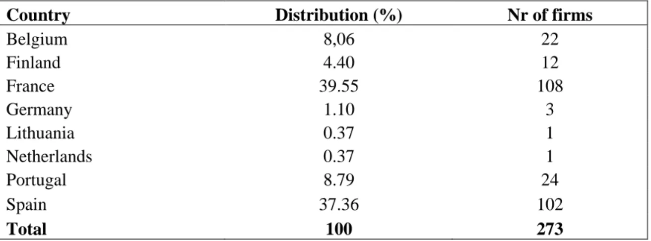
The final sample has 273 firms from different countries in the euro zone. There are firms from Belgium, Finland, France, Germany, Lithuania, Netherlands, Portugal and Spain. The distribution of firms per country is as shown in Table 1.

(35)

Table 1 – Firms’ distribution by country

Country Distribution (%) Nr of firms

Belgium 8,06 22 Finland 4.40 12 France 39.55 108 Germany 1.10 3 Lithuania 0.37 1 Netherlands 0.37 1 Portugal 8.79 24 Spain 37.36 102 Total 100 273

3.3.2. Variables and firm characterization statistics

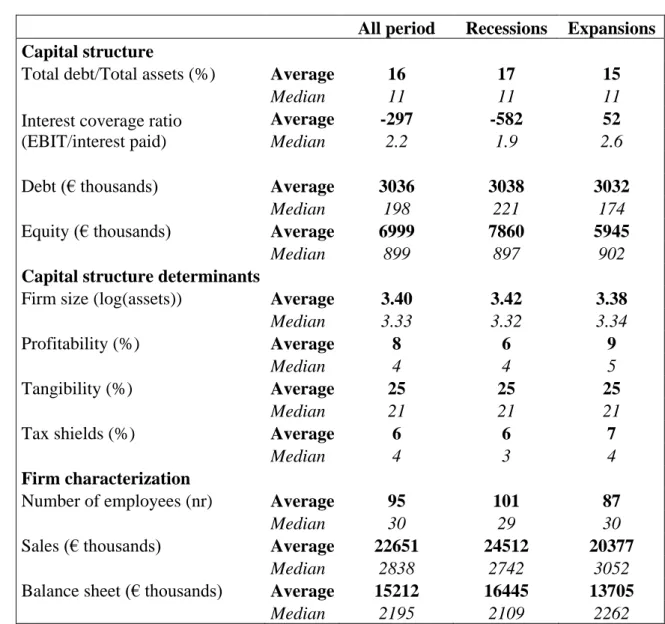
In this section we present firms’ main statistics that characterize our sample. Table 2 presents the statistics for the main variables used in this study, such as leverage, firm size, profitability, tangibility, and non-debt tax shields on the capital structure and determinants dimensions. The firm size indicators provide a deeper knowledge of the type of firms contained in this sample with statistics for the number of employees, sales and balance sheet size.

(36)

Table 2 - Sample summary statistics

All period Recessions Expansions Capital structure

Total debt/Total assets (%) Average 16 17 15

Median 11 11 11

Interest coverage ratio (EBIT/interest paid)

Average -297 -582 52

Median 2.2 1.9 2.6

Debt (€ thousands) Average 3036 3038 3032

Median 198 221 174

Equity (€ thousands) Average 6999 7860 5945

Median 899 897 902

Capital structure determinants

Firm size (log(assets)) Average 3.40 3.42 3.38

Median 3.33 3.32 3.34

Profitability (%) Average 8 6 9

Median 4 4 5

Tangibility (%) Average 25 25 25

Median 21 21 21

Tax shields (%) Average 6 6 7

Median 4 3 4

Firm characterization

Number of employees (nr) Average 95 101 87

Median 30 29 30

Sales (€ thousands) Average 22651 24512 20377

Median 2838 2742 3052

Balance sheet (€ thousands) Average 15212 16445 13705

Median 2195 2109 2262

The table shows the statistics for capital structure indicators such as leverage, debt and equity. Leverage is measured by the ratio of total debt to total assets and the interest coverage ratio (EBIT/interest paid). Debt and equity are measured respectively by total debt and total equity. The table also shows the statistics for the capital structure determinants: firm size (Logarithm of total assets), profitability (EBIT to Total assets), tangibility (Tangible assets to Total assets) and non-debt tax shields (Depreciation to Total assets). For firm characterization we present the average and median values for the number of employees, sales and balance sheet size.

3.3.3. Business cycle

The business cycle effect is captured in the study by the use of the output gap as a synthetic measure of the economic conditions. In the regressions we use the output gap and, alternatively, a dummy that takes the value one when there is an expansion and zero when there is a recession. Figure 2 shows the output gap for the entire period between 1996 and 2015. During this period, in the euro area, recessions are observed in eleven years and expansions in nine years. This data indicates that most of the years

(37)

show a negative output gap mainly due to international crises such as the dotcom bubble with the recession in 2003, the international financial crisis of 2008 and the consequent sovereign debt crisis in the euro area in 2010.

Figure 2 - Evolution of the Eurozone output gap

-4 -3 -2 -1 0 1 2 3 4

Eurozone Output gap