Dynamic behaviour of a steel composite frame railway bridge

D

YNAMIC BEHAVIOUR OF A STEEL

COMPOSITE FRAME RAILWAY BRIDGE

B

B

C

M

Dissertação submetida para satisfação parcial dos requisitos do grau de

MESTRE EM ENGENHARIA CIVIL —ESPECIALIZAÇÃO EM ESTRUTURAS

Orientador: Professor Doutor Rui Artur Bártolo Calçada

Coorientador: Prof. Dr.-Ing. Benno Hoffmeister

M

I

E

C

2015/2016

DEPARTAMENTO DE ENGENHARIA CIVIL

Tel. +351-22-508 1901 Fax +351-22-508 1446

 miec@fe.up.pt

Editado por

FACULDADE DE ENGENHARIA DA UNIVERSIDADE DO PORTO

Rua Dr. Roberto Frias 4200-465 PORTO Portugal Tel. +351-22-508 1400 Fax +351-22-508 1440  feup@fe.up.pt  http://www.fe.up.pt

Reproduções parciais deste documento serão autorizadas na condição que seja mencionado o Autor e feita referência a Mestrado Integrado em Engenharia Civil - 2015/2016 - Departamento de Engenharia Civil, Faculdade de Engenharia da Universidade do Porto, Porto, Portugal, 2016.

As opiniões e informações incluídas neste documento representam unicamente o ponto de vista do respetivo Autor, não podendo o Editor aceitar qualquer responsabilidade legal ou outra em relação a erros ou omissões que possam existir.

To my parents and brothers

“Believe you can and you’re halfway there” Theodore Roosevelt

ACKNOWLEDGMENTS

The work which constitutes this thesis was only possible due to the contribution of some people. To all who have accompanied me during this journey, and to those who in some way contributed to their achievement, I express my sincere gratitude. For the importance of their role, I present my special thanks:

 First of all, to Prof. Dr. Ing. Benno Hoffmeister for the warm reception and for enable the desire to do this work at RWTH Aachen to become a reality. For the availability and for all the help, providing me with all the necessary resources and all the scientifical staff connections;

 To Professors Dr.-Ing. Daniel Pak and to Dipl. Ing. Hetty Bigelow, for their support and availability, for providing me with the opportunity to participate in research projects, allowing me to integrate a research group and getting in touch with real engineering problems. For their help processing all the data and for providing me with the opportunity to conduct numerical studies on a real railway bridge;

 To Professor Dr. Rui Calçada for the availabilty, since the first moment, helping me finding a supervisor at RWTH Aachen, as well as for the help in choosing the field of work to this thesis. For the support, encouragement and for his fully availability, even when he was extremely busy;

 To the high speed research group of the Civil Engineering Department of FEUP, especially to the engineer Joel Pedro Malveiro, for the precious and tireless support in all the questions related to the ANSYS, without whom would not have been possible to complete the numerical model. Also thank to Pedro Jorge throughout the bibliography provided, Andreia Meixedo and Cristiana Bonifácio who provided promptly their numerical models, that were important to better understand the functioning of ANSYS;

 To all the friends who accompanied me over these five years, for all the support, affection, friendship and motivation. To the friends who I had the opportunity to meet in these five months in Aachen, that were undoubtedly important in this experience;

 To Sofia, for all the affection, dedication, patience and constant support over the past couple years and for the trust that she has always had in me;

 Finally I would like to thank to those whom I owe everything, my family. To my mother, Susana, for being the engine of our home and for taking care of me with the greatest love and affection from the first day. To my father, Ivo, the best example I have of determination, for all his support and wise words at the right time. To my brothers, Helena e Guilherme, for the encouragement and love, and for everything they symbolize in my life.

ABSTRACT

This thesis primarily aims to study the dynamic behaviour of a bridge over the Salzach river, under the action of railway traffic. The bridge in focus, is located in the Austrian state of Salzburg, and is part of the ÖBB1 _{conventional railway line Salzburg-Schwarzach/St.V.-Wörgl, between 65.439 km and 65.485} km, with a steel composite cross-section consisting of two traffic routes supported by two single span structures.

Initially, this study consisted on a research of other papers on railway bridges, as a way to understand its singularities, and a detailed analysis of the regulation on the design of railway bridges (Standards EN1991-2 and EN1990-AnnexA2), in order to understand the major design criteria of railway bridges. From these became clear the importance of the structural safety, track safety and passengers comfort. Consequently, several methodologies of dynamic analysis were studied, from which stood out the numerical ones, since they have a wider application field.

The numerical model of the structure is described, model which was developed with the finite elements software ANSYS, where the modal analysis was carried out. In a first phase, the numerical model of the bridge does not consider neither the ballast nor the rails, once during the experimental tests, the bridge was not yet completed, thereby intending the model to reproduce as faithfully as possible the actual conditions under which the experimental tests were performed. The experimental tests performed under the experimental campaign are also described, as well as the results obtained.

Thus, as regard the study of the bridge in question, the experimental tests carried out on the bridge, allowed to obtain results that were compared with those obtained using the numerical model built in ANSYS, particularly the frequencies and the vibration modes.

In a second phase, the ballast, sleepers and railway tracks were added to the previous numerical model, in order to allow an analysis using moving loads modelling, thus simulating the passage of a train on the bridge. Therefore, using the load model of a real train, IC (Intercity Train) belonging to Deutsche Bahn AG, a German railway company, and being known its geometry and axle loads, it was possible to run a dynamic analysis using moving loads, through the MATLAB programme.

KEYWORDS:train, railway bridge, modelling, dynamic analysis, moving loads.

RESUMO

A presente dissertação tem como objetivo primordial estudar o comportamento dinâmico de uma ponte sobre o rio Salzach, sob a ação de tráfego ferroviário. A ponte situa-se na Áustria, no estado de Salzburgo, na Linha Convencional Salzburg-Schwarzach/St.V.-Wörgl, entre o km 65,439 e o km 65,485, sendo uma estrutura mista constituída por duas vias de circulação suportadas por dois tabuleiros independentes.

Inicialmente, o estudo envolveu uma pesquisa de outros trabalhos sobre pontes ferroviárias, de forma a compreender as suas particularidades, e uma análise detalhada à regulamentação em vigor para o dimensionamento de pontes ferroviárias (normas EN1991-2 e EN1990-AnnexA2), com o objetivo de perceber os principais critérios do dimensionamento de pontes inseridas em linhas ferroviárias. Destas normas tornou-se clara a importância da verificação da segurança estrutural, segurança da via e o conforto dos passageiros. Consequentemente, várias metodologias de análise dinâmica foram analisadas, de entre as quais se destacaram as numéricas, devido ao campo de aplicação mais alargado. Descreve-se o modelo numérico da ponte em estudo, desenvolvido no programa de cálculo em elementos finitos ANSYS, que permitiu fazer as análises modais. Numa primeira fase, o modelo numérico da ponte não contempla nem balastro nem a ferrovia, uma vez que aquando dos testes experimentais, a ponte ainda não se encontrava concluída, pretendendo assim o modelo reproduzir o mais fielmente as condições reais em que os testes experimentais foram realizados. São também descritos os ensaios experimentais realizados no âmbito da campanha experimental, bem como os resultados obtidos.

Assim, no que diz respeito ao estudo da ponte em questão, os testes experimentais levados a cabo na ponte permitiram obter resultados que foram comparados com os obtidos recorrendo ao modelo numérico construído no ANSYS, nomeadamente frequências e modos de vibração.

Numa segunda fase, foram adicionados ao modelo anterior, o balastro e a ferrovia, de modo a permitir uma análise dinâmica recorrendo a cargas móveis, simulando assim a passagem de um comboio na ponte. Então, utilizando o “Load Model” de um comboio real, IC (Intercity Train), pertencente à Deutsche Bahn AG, uma companhia ferroviária alemã e, sendo conhecidas a sua geometria e cargas por eixo, foi possível efetuar uma análise dinâmica recorrendo a cargas móveis, recorrendo ao programa MATLAB.

KURZFASSUNG

Das Hauptziel dieser Abschlussarbeit ist die Untersuchung des dynamischen Verhaltens infolge Zugüberfahrten der Eisenbahnbrücke über die Salzach. Die betrachtete Brücke befindet sich im österreichischen Bundesland Salzburg und ist Teil der ÖBB Strecke Salzburg-Schwarzach/St.V.-Wörgl, zwischen km 65,439 und km 65,485; sie besteht aus Stahl-Verbundquerschnitten wobei zwei Einfeldstrukturen jeweils ein Gleis tragen.

Grundlage der Arbeit bildete eine Literaturrecherche zum Thema Eisenbahnbrücken, um die Besonderheiten der untersuchten Brücke zu verstehen, sowie eine Auseinandersetzung mit den gültigen Regelwerken zur Brückenbemessung (DIN EN1991-2 und DIN EN1990-Anhang A2), um die Hauptdesignkriterien bei der Brückenbemessung zu verstehen. Die Bedeutung der Tragsicherheit, der Gleislagestabilität und des Reisendenkomforts wurde ersichtlich. Mehrere Methoden der dynamischen Berechnung wurden untersucht, wobei hier die numerischen Verfahren aufgrund ihres größeren Anwendungsgebietes herausstehen.

Das numerische Model der Brücke wird beschrieben; das Modell wurde mit der Finite-Elemente (FE-) Software ANSYS erstellt zur Durchführung dynamischer Berechnungen. In der Anfangsphase werden beim Modell weder Schotter noch Schienen berücksichtigt, da während der ersten Vergleichsmessung an der Brücke diese noch nicht vollständig fertiggestellt war. Daher sollte das Modell die tatsächlichen Gegebenheiten realistisch darstellen. Die durchgeführten Messungen werden ebenfalls beschrieben und die Messergebnisse vorgestellt.

Die Messergebnisse wurden mit den Berechnungsergebnissen verglichen, welche mit dem numerischen Modell in ANSYS erstellt wurden, im Fokus standen dabei Frequenzen und Modalformen.

In der zweiten Phase wurden Schotter, Schwellen und Schienen im Modell ergänzt, um dynamische Berechnungen mit bewegten Lasten zu ermöglichen, um so Zugüberfahrten zu simulieren. Es wurde das Modell eines realen Zuges IC (Intercity) der Deutsche Bahn AG verwendet, da von diesem Achslasten und -abstände bekannt waren.

TABLE OF CONTENTS ACKNOWLEDGMENTS ... I ABSTRACT ... III RESUMO ... V KURZFASSUNG ... VII

1 INTRODUCTION ... 1

1.3.STRUCTURE OF THE WORK ... 7

2 BIBLIOGRAPHICAL SURVEY ... 9

2.1.INTRODUCTION ... 9

2.2.RESONANCE PHENOMENA ... 9

2.2.1.MECHANISM OF RESONANCE AND CANCELLATION FOR TRAIN-INDUCED VIBRATIONS ON BRIDGES ...10

2.2.2.BRIDGE RESONANCE INDUCED BY MOVING LOAD SERIES ...12

2.2.2.1. Bridge resonance induced by periodically loading of moving load series ...14

2.2.2.2. Bridge resonance induced by loading rate of moving load series ...14

2.2.3.BRIDGE RESONANCE OWING TO THE SWAY FORCES OF TRAIN VEHICLES ...15

2.3.FACTORS INFLUENCING THE DYNAMIC RESPONSE OF THE STRUCTURE ... 15

2.3.1.BEARINGS STIFFNESS ...16

2.3.2.TRAIN-BRIDGE INTERACTION ...17

2.3.3.DISTRIBUTION OF THE LOADS THROUGH THE SLEEPERS AND BALLAST LAYER ...20

3 DESIGN CODES APPLIED TO RAILWAY BRIDGES ... 23

3.1.INTRODUCTION ... 23

3.2.ACTIONS TO BE CONSIDERED... 23

3.2.1.STATIC EFFECTS ...23

3.2.1.1. Load Model 71...24

3.2.1.2. Load Models SW/0 and SW/2 ...25

3.2.1.3. Load Model “Unloaded Train” ...26

3.2.1.4. Consideration of Dynamic Effects in Static Analysis ...26

3.2.2.1. Requirements for a static or dynamic analysis ...30

3.2.2.2. Requirements for a dynamic analysis...31

3.2.2.3. Speeds to be considered ...36

3.2.2.4. Bridge Parameters...36

3.3.VERIFICATIONS OF THE LIMIT STATES ... 40

3.3.1.STRUCTURAL SAFETY ...40

3.3.2.TRAFFIC SAFETY ...41

3.3.2.1. Vertical acceleration of the deck ...41

3.3.2.2. Vertical deformation of the deck ...43

3.3.3.PASSENGER COMFORT ...43

4 METHODOLOGIES FOR DYNAMIC ANALYSIS ... 47

4.1.INTRODUCTION ... 47

4.2. DYNAMIC ANALYSIS WITHOUT TRAIN-BRIDGE INTERACTION ... 48

4.2.1.DYNAMIC EQUILIBRIUM OF A STRUCTURE ...48

4.2.2.CONTRIBUTION OF MOVING LOADS ...49

4.2.3.RESOLUTION OF DYNAMIC EQUILIBRIUM EQUATION ...50

4.2.3.1. Direct Numerical Integration ...50

4.2.3.2. Mode Superposition Method ...52

4.2.4.MOVING LOADS METHODOLOGY WITH ANSYS-MATLAB INTERACTION ...53

4.2.4.1. Modal analysis...54

4.2.4.2. Extraction of the modal values of the quantities to be analysed ...54

4.2.4.3. Extraction of the modal vertical displacements of the railway nodes ...54

4.2.4.4. Dynamic analysis ...54

4.3. DYNAMIC ANALYSIS WITH TRAIN-BRIDGE INTERACTION ... 55

4.3.1.ITERATIVE METHODOLOGY ...56

5 EXPERIMENTAL CHARACTERIZATION AND NUMERICAL

MODELLING OF THE SALZACH RIVER BRIDGE ... 59

5.1.INTRODUCTION ... 59

5.2.BRIDGE OVER THE SALZACH ... 60

5.2.1.CHARACTERIZATION AND GEOMETRIC PROPERTIES OF THE STRUCTURE ...61

5.2.1.1. Sleepers ...63

5.2.1.3. Rails ...65

5.2.2.GROUND CONDITIONS FOR PILE FOUNDATION ...65

5.3.FINITE ELEMENT NUMERICAL MODEL ... 67

5.3.1.NUMERICAL MODEL A ...67

5.3.1.1. Finite Element Types used ...69

5.3.1.2. Properties assigned to the elements (Real Constants) ...70

5.3.1.3. Materials used in modelling ...75

5.3.1.4. Construction of the numerical model A ...75

5.3.2.NUMERICAL MODEL B ...79

5.3.2.1. Finite Element Types used ...79

5.3.2.2. Properties assigned to the elements (Real Constants) ...80

5.3.2.3. Materials used in modelling ...80

5.3.2.4. Construction of the numerical model ...81

5.4.MONITORING SYSTEM ... 85

5.4.1.OBJECTIVES AND INSTALLATION ...85

5.4.2.INSTRUMENTATION AND DATA ACQUISITION SYSTEM FOR THE DYNAMIC MEASUREMENTS ...85

5.4.3.MONITORING RESULTS ...91

5.5.MODAL ANALYSIS OF THE BRIDGE OVER THE SALZACH RIVER ... 93

6 DYNAMIC ANALYSIS OF THE BRIDGE OVER THE

SALZACH RIVER ... 99

6.1.INTRODUCTION ... 99

6.2.MOVING LOADS METHODOLOGY ... 99

6.3.STUDY OF PARAMETERS TO USE IN THE DYNAMIC ANALYSIS ... 103

6.3.1.SPEEDS TO BE CONSIDERED ...103

6.3.2.TIME INCREMENT ...103

6.3.3.INFLUENCE OF THE DAMPING COEFFICIENT IN THE DYNAMIC RESPONSE OF THE STRUCTURE ...104

6.3.4.INFLUENCE OF THE NUMBER OF VIBRATION MODES IN THE RESPONSE OF THE STRUCTURE ...105

6.3.4.1. Influence in terms of accelerations ...105

6.3.4.2. Influence in terms of displacements ...107

7 CONCLUSIONS AND FUTURE RESEARCH ... 111

7.1.CONCLUSIONS ... 111

Bibliographic References ... 115

ANNEX A1 APDL CODE TO GENERATE NUMERICAL

LIST OF FIGURES

Fig. 1.1 - EU27 Share of CO2 emissions from fuel combustion [4] ... 3

Fig. 1.2 - High Speed system in Europe [8]: a) by 2010; b) by 2025. ... 5

Fig. 2.1 - Observation of the resonance effects in a simply supported bridge [10] ...10

Fig. 2.2 - Observation of the cancellation effects in a simply supported bridge [10] ...11

Fig. 2.3 - Overlapping responses in free vibration of a simply supported bridge, after the passage of forces equally spaced of 26.4 m, with speed of: a) 253 km/h; b) 192 km/h [10] ...12

Fig. 2.4 - Sources of errors [11] ...16

Fig. 2.5 - Moving loads model [13] ...17

Fig. 2.6 - Acceleration in the mid-span: with and without interaction [15] ...17

Fig. 2.7 - Reduction of the impact coefficients (R) and maximum accelerations (R’) for bridges [13] ...19

Fig. 2.8 - Intensities of reduction for the impact coefficients (γ) and for the maximum accelerations (γ’) [13] ...19

Fig. 2.9 - Distribution of the axle loads through the sleepers and ballast layer [13] ...20

Fig. 2.10 - Maximum accelerations in bridges of span: 𝐿 = 5 𝑚 and 𝐿 = 10 𝑚 [13] ...21

Fig. 3.1 - Load Model 71 and characteristic values for vertical loads [16] ...24

Fig. 3.2 - Loads Distribution to obtain maximum bending moment at mid-span of the central section, in a continuous deck with 5 main sections [18] ...24

Fig. 3.3 - Load Models SW/0 and SW/2 [16] ...25

Fig. 3.4 - Limits of bridge natural frequency n0 (Hz) as a function of L (m): (1) Upper limit of natural frequency; (2) Lower limit of natural frequency [16] ...28

Fig. 3.5 - Flow chart for determining whether a dynamic analysis is required [16] ...30

Fig. 3.6 - Articulated train (Example: Eurostar) [16] [18] ...31

Fig. 3.7 - Conventional train (Example: ICE) [16] [18] ...32

Fig. 3.8 - Regular train (Example: Talgo) [16] [18] ...32

Fig. 3.9 - Dynamic signatures (zero damping) for European high speed trains [18] ...33

Fig. 3.10 - Load Model HSLM-A [16] ...34

Fig. 3.11 - Load Model HSLM-B [16] ...35

Fig. 3.12 - HSLM-B: determination of the number N of concentrated loads and the spacing d between loads [16] ...35

Fig. 3.13 - Damping as a function of span [18] ...38

Fig. 3.14 - Additional damping ∆ζ [%] as a function of span length L [m] [16] ...39

Fig. 3.15 - Variation in amplification factor of ballast acceleration at sleeper ends/bridge deck acceleration without a ballast mat [14] ...42

Fig. 3.16 - Variation in amplification factor of ballast acceleration [18] ...42

Fig. 3.17 - Maximum permissible vertical deflection (δ) for railway bridges with 3 or more successive simply supported spans corresponding to a permissible vertical acceleration of 𝑏𝑣 = 1,0 𝑚/𝑠2 in a coach for speed V (km/h) [17]...44

Fig. 4.1 - Variation of Load Function on a node k due to the passage of the load 𝑃𝑟 [20] ...50

Fig. 4.2 - Resultant displacement and modal components ...52

Fig. 4.3 – Steps involved in the implementation of the moving loads methodology [adapted from 24] .54 Fig. 4.4 - Vehicle-Structure interaction model [25] ...55

Fig. 5.1 – Location of the Salzach bridge: a) aerial view [29]; b) aerial view – project. ...60

Fig. 5.2 – Longitudinal section Salzach Bridge ...61

Fig. 5.3 – Salzach Bridge without backfill and installations – side view ...61

Fig. 5.4 – Steel beams – inside view ...62

Fig. 5.5 – Typified cross-section at the abutment ...62

Fig. 5.6 – Deck Cross-section...63

Fig. 5.7 – Dimensions of the modelled sleepers: a) – geometry representation [20]; b) – photo in the construction site. ...64

Fig. 5.8 – Baseplate behaviour with isotropic (a) and orthotropic (b) material [20] ...64

Fig. 5.9 – Detail of retaining wall founded on piles ...66

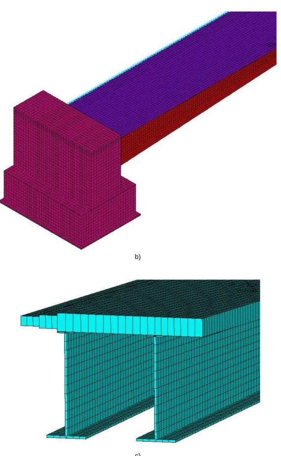
Fig. 5.10 – Overview of the Numerical Model A: a) – general overview; b) – mesh zoom; c) – transversal cut...68

Fig. 5.11 – Detail of the different thickness of the concrete slab: a) Perspective view; b) Transversal profile. ...71

Fig. 5.12 – Spring applied at the bottom of the abutments: a) transversal view; b) perspective view. ..72

Fig. 5.13 – General scheme of the applied springs ...73

Fig. 5.14 – Finite Element Mesh: a) – abutment; b) – steel beams; c) – concrete deck. ...76

Fig. 5.15 – Modelling of the connection areas applying MPC 184 elements ...77

Fig. 5.16 – Connection between the bridge structure and the abutments (through coincident nodes): a) – transversal view; b) – perspective view; c) – zoom of common points. ...78

Fig. 5.17 – Overview of the Numerical Model B ...79

Fig. 5.18 – Overview of the Numerical Model B ...81

Fig. 5.19 – Detail: Sleepers, baseplates and rails ...82

Fig. 5.20 – Modelling of the connection areas applying MPC 184 elements: a) – transversal view right; b) – perspective view left. ...84

Fig. 5.21 – Salzach Bridge without backfill and installations: a) Wörgl side view; b) Salzburg side view. ...85

Fig. 5.23 – General overview of a measurement point ...86

Fig. 5.24 – Equipment used in the measurements: a) – recording device; b) – switch; c) – sensor. ....87

Fig. 5.25 – General overview scheme of the installation of the measurement points ...88

Fig. 5.26 – General overview of the installed measurement points ...89

Fig. 5.27 – General overview scheme of the location of the hydraulic accurator ...89

Fig. 5.28 – Examples of mode shapes obtained through the different positions of the hydraulic accurator: a) – results from position A; b) – results from position B. ...90

Fig. 5.29 – Hydraulic accurator: a) - general view; b) – enlarged view. ...90

Fig. 5.30 – Shifted data obtained from measurements: a) – example of transversal acceleration; b) – example of longitudinal acceleration. ...91

Fig. 5.31 – Detrend function: a) – constant; b) – linear; c) – adaptive. ...92

Fig. 5.32 – Corrected data after using the adaptive detrend function: a) – example of transversal acceleration; b) – example of longitudinal acceleration. ...92

Fig. 5.33 – Deformed shape of the prominent vibration modes in the response of the deck ...96

Fig. 6.1 – IC Train (Intercity Train) – Deutsche Bahn AG ...100

Fig. 6.2 – Initial KeyPoints of the loads path ...102

Fig. 6.3 – Maximum acceleration values at mid-span in function of the speed and ∆𝑡 ...104

Fig. 6.4 – Maximum acceleration values at mid-span for the damping coefficient ...105

Fig. 6.5 – Acceleration at mid-span in the numerical model B, with the train circulating at a speed of 150 km/h: a) – 30 Hz; b) 60 Hz. ...106

Fig. 6.6 – Maximum and minimum acceleration values at mid-span due to an IC train crossing the bridge (limit of frequencies of 30 Hz and 60 Hz) ...107

Fig. 6.7 – Displacement at mid-span in the numerical model B, with the train circulating at a speed of 150 km/h: a) – 30 Hz; b) 60 Hz. ...108

Fig. 6.8 – Maximum and minimum displacement values at mid-span due to an IC train crossing the bridge (limit of frequencies of 30 Hz and 60 Hz) ...109

LIST OF TABLES

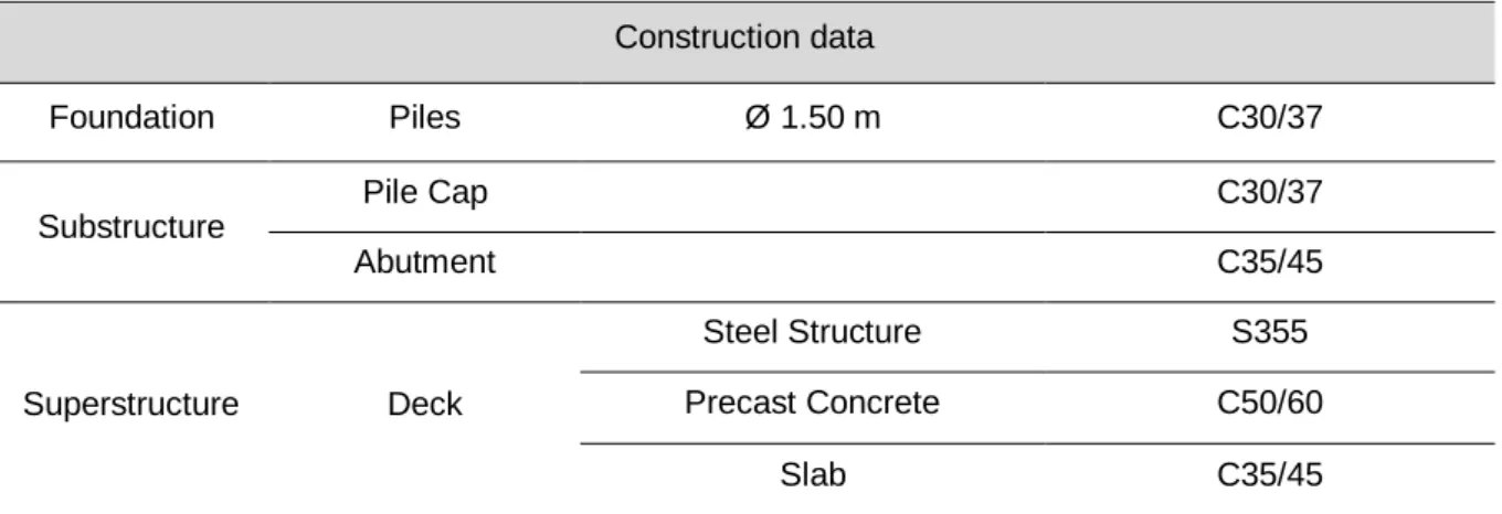
Table 1.1 - Carbon footprint of transport services [2]: a) High Speed Rail Transport; b) Road Transport; c) Air Transport. ... 2 Table 1.2 - EU27 transport modal share [4] ... 4 Table 3.1 - Characteristic values for vertical loads for Load Models SW/0 and SW/2 [16] ...25 Table 3.2 - HSLM-A characteristics [16] ...34 Table 3.3 - Values of damping to be assumed for design purposes [16] ...38 Table 3.4 - Maximum permitted peak values of bridge deck acceleration [17] ...41 Table 3.5 - Maximum permitted peak values of bridge deck acceleration ...43 Table 3.6 - Recommended levels of comfort [17] ...43 Table 4.1 - Numerical methodology scheme that considers the train-bridge interaction [adapted from 19] ...57 Table 5.1 – UIC 60 rail properties [20] ...65 Table 5.2 – Soil parameters ...65 Table 5.3 – Construction data ...66 Table 5.4 – Element Types used in Model A ...69 Table 5.5 – Characteristics of Elements BEAM 44 ...70 Table 5.6 – Characteristics of Elements SHELL 63 ...71 Table 5.7 – Axial stiffness of each concrete pile ...74 Table 5.8 – Stiffness of the springs ...74 Table 5.9 – Stiffness of the springs in vertical and horizontal directions ...74 Table 5.10 – Young’s modulus of concrete at measured construction levels ...75 Table 5.11 – Element Types used in Model B ...80 Table 5.12 – Materials considered in the model B modelling ...81 Table 5.13 – Measured eigenfrequencies values ...93 Table 5.14 – Eigenfrequencies values obtained through the numerical model A ...94 Table 5.15 – Eigenfrequencies values obtained through the numerical model A ...97 Table 6.1 – Loads per axle in the IC Train ...100 Table 6.2 – Initial coordinates of the rails ...102 Table 6.3 – Values of damping to be assumed for design purposes [16] ...102 Table 6.4 – Recommended time increments ...104

1

INTRODUCTION

1.1. CONSIDERATIONS

The increasing globalization of the market, with the movement of people and goods exceeding the geographical limits of each country, highlights the need for faster and more efficient transport services. The rail transport, in particular the high-speed, presents, today, with great potential to fulfil the society needs and as an advantageous alternative compared to road and air transport. The main advantages occur at the level of transportation costs, capacity, safety and comfort [1]. The development and expansion of high-speed lines allowed to shorten travel times and contributed to the social development and economic growth, particularly in Europe, whose geography is in favour of this type of transport.

Moreover, the environmental respect, nowadays, is a factor with huge importance. Comparing the carbon footprint of which one of these means of transport – including not only the operation phase and the energy provision, but also the infrastructure (track system, motorways, airports) and the construction of rolling stock, cars and airplanes – it is possible to conclude that, in fact, the high speed rail transport is far away more “eco-friendly”.

Table 1.1 shows a comparison between high speed train, air transport and road, in a comparable geographic context: for the same route from Valence to Marseille. Concerning to the road, the study represents a section of A7 motorway from Valence to Marseille, with the following characteristics: length of 210 kilometres; high traffic estimate of 58,400 vehicles (including all vehicles categories) per day in 2004; 2x3 lanes infrastructure. Regarding the air transport, on a normal day, around 100 to 120 planes land in the Airport of “Marseille Provence”; in 2004 a total of 86,000 planes movement has been observed between the two cities. The distance between the center of Valence and Marseille Airport is 170 km, and the annual traffic was around 5.6 million passengers in 2004. About the high speed train, the “LGV Méditerranée” (Valence – Marseille) has a total length of 250 km and in 2004 transported 20.4 million passengers [2]. The comparison between the three transport modes is done on the unit of passenger kilometre.

Table 1.1 - Carbon footprint of transport services [2]: a) High Speed Rail Transport; b) Road Transport; c) Air Transport.

a)

High Speed Rail Transport

Main assumptions

Rolling Stock 1.0 g CO2/ pkm Lifespan 30 years, 18 trains in operation

Operation 5.7 g CO2 / pkm

French electricity mix, 24.1 kWh per train kilometre, 40 880 trains a year, 20.4 millions of passengers a

year Construction

of High Speed Line

4.3 g CO2 / pkm

20.4 millions of passengers a year, 250 km of length (10 km tunnels, 2.7 km covered trenches, 16 km on

viaducts, 20.3 km of bridges) Grand Sum 11.0 g CO2 / pkm b) Road Transport Main assumptions Car Construction 20.9 g CO2/ pkm

Overall transport performance of 150,000 km, average load factor 1.6, weight of the car: 1310 kg Operation 130 g CO2 / pkm

Average consumption of 7 litres of gasoline for 100 km, load factor of 1.6 passengers

Road 0.7 g CO2 / pkm

2*3 lanes between Valence and Marseille, transport performance of 56,000 cars, load factor of 1.6

passengers, share of freight: 65.5% Grand Sum 151.6 g CO2 / pkm c) Air Transport Main assumptions Airplane Construction 0.5 g CO2/ pkm

Airbus A 320 with 320 seats, empty weight 61 t (mainly aluminium)

Operation 163.2 g CO2 / pkm

Load factor: 65%, Consumption per Ton-kilometre: 452 g kerosene, 100 kg for one passenger including luggage Airport

Construction 0.3 g CO2 / pkm

Allocation to passenger-traffic: 90%, around 600ha for runways, building and equipment

Among all sectors, the transport sector is the only one in which the CO2 emissions are continuing to increase, in spite of all technological advances. Furthermore, transport emissions in Europe increased by 25%, between 1990 and 2010, while, on the other hand, the emissions from the energy and industrial sectors has been declining over the time [3]. Hence, it is important to make a transition to a more sustainable transport system in order to reduce the values of emissions due to transport means.

According to Figure 1.1, a large part of CO2 emissions is due to the role of transports. Comparing the different types of transport, it is clear that the rail is one of the least responsible for these numbers and, therefore, it has almost no impact on the CO2 emissions. Thus, rail need to be given more attention because of its crucial role as an important part of the solution, playing a leading role in reducing the transport related emissions and to contribute to the climate protection.

Fig. 1.1 - EU272 _{Share of CO}

2 emissions from fuel combustion [4]

Once knowing that the train is the vehicle that has less impact on the environment, it would be to expect this to be the most popular mean of transport. However, this does not occur, neither the transport of persons nor freight. The most responsible for the transport of passengers is the car, with a rate of 83.6%, according to data from UIC3 (2015), followed by aircraft and only after by the train. Concerning the transport of freight, the road and the navigation appear with a similar prevalence, although the road still have a higher percentage, appearing the train as the third mode of transport (Table 1.2).

2_{Members of the European Union as of the 2007 expansion (inclusion of Romania and Bulgaria)} 3_{International Union of Railways}

Electricity and Heat 38.6% Manufacturing 14.3% Residential 10.1% Other 4.5% _{Agriculture, Forestry} and Fishing 1.5% Road 70.9% Navigation 14.4% Aviation 12.6% Rail 1.5% Other transport 0.6% Transport 31%

Table 1.2 - EU27 transport modal share [4] Passenger (passenger-km) Freight (tonne-km) Total (TU) Road 83.6 % 46.9 % 70.3 % Aviation 8.8 % 0.1 % 5.7 % Navigation 0.6 % 41.9 % 15.5 % Rail 7 % 11.1 % 8.5 %

The railway transport, in particular the high speed, can play a key role in this context, contributing to the purposes of integration and sustainable development of countries, either in terms of economic growth, or in terms of social development. This type of transport is particularly competitive for distances from 300 km to 1000 km [5], providing shorter journey times and greater comfort, when compared to air and road transports. Therefore, the European geography fits in these conditions, once the major urban centres are spaced in such distances.

In Europe, the first high speed lines were built in the 1980s and 1990s, improving travel times and, since then, several countries have built extensive high speed networks, existing now several cross-border high speed rail links [6]. In order to European Union to become a success with a thriving economy, goods and people need to be able to circulate rapidly and easily between member states, and even beyond. Consequently, it is in that context that the Trans-European High Speed Rail Network (TEN-R) comes up, which main objective is to achieve the interoperability of the European high speed train network at the various stages of its design, construction and operation [7].

As shown on Figure 1.2, nowadays the high speed railways are already distributed throughout Europe and it is expected, in a near future, the significant increase in the number of kilometres in operation.

a)

b)

Due to being subjected to high intensity moving loads, railway bridges are structures where the dynamic effects are always present, reason why the dynamic behaviour of a bridge must always be considered in its design.

These effects are of even greater importance when associated with the development and progress of high speed, thus leading to the rise of new challenges, in terms of the dynamic behaviour of structures built in the respective routes, subjected to certain actions, distinct of those who were verified on conventional lines. It was found that, in many situations, the traffic of vehicles at significant higher speeds (above 200 km/h) on the same structure, raised different dynamic effects of those previously known, with relevance to the resonance effects.

Therefore, emerged the need to study the phenomena associated with behaviours never before experienced and, through its conclusions, implementing European standards with procedures and checks, covering the recent developments, in order to be considered in the structural design of new bridges, or in the reinforcement of existing structures.

Despite being a well explored field, it continues to be very interesting and important to conduct research works on railway bridges throughout Europe, enabling the understanding of their behaviour towards current and potential actions on structures.

The main purpose of this assignment is to investigate the performance of a steel composite frame Railway Bridge, by means of measurements in a particular bridge, under construction, in Sankt Johann Im Pongau, in the state of Salzburg in Austria, to assess and validate his behaviour when subjected to intense railway traffic.

In Civil Engineering, the evaluation process of structures is often performed using numerical models to reproduce the properties of the structure and to predict his behaviour over time. The uncertainty that exists in defining these properties implies experimental studies on existing structures, and posterior calibration of the numerical models, based on the measured information. Thus, with the use of numerical models - to reproduce realistically the complexity of the track-bridge system - combined with the measured information obtained experimentally, it is possible to develop a complex and advanced study of the bridge. It is then possible, in addition to verify the suitability of the structure at high speed, to obtain enough information to identify common behaviours of the structure, that contribute to future studies and regulations, in order to provide a better design of new structures in the future.

1.2. OBJECTIVES

Inserted in a research project carried out by the Institute for Steel Structures of the RWTH Aachen University (Institut und Lehrstuhl für Stahlbau Leichtmetallbau Prof. Dr. –Ing. Markus Feldmann), this work aims to study the dynamic behaviour of a steel composite frame railway bridge in Schwarzach-Sankt Veit im Pongau, a market town in the Schwarzach-Sankt Johann im Pongau district, in the Austrian state of Salzburg.

Thus, in practical terms, the dynamic study of the bridge involves the development of a numerical model using the finite element method, covering all the bridge elements, from the deck and the track, to the foundations. Subsequently, it is intended to validate the numerical model with experimental results, resulting from a campaign of experimental tests carried out on the bridge.

Another objective is also to perform parametric studies to understand the influence of various parameters on the dynamic properties of the structure and study the modal parameters of the structure (such as frequencies and vibration modes).

Finally, it is intended to study the dynamic response of the structure when this is subjected to the passage of an Intercity train.

1.3. STRUCTURE OF THE WORK

This thesis is divided into seven chapters, whose content is briefly summarized in the following paragraphs.

The present Chapter 1 presents the main motivations for the development of this thesis, describes its main objectives, and outlines the organization of the text.

A bibliographical survey of previous researches concerning dynamic behaviour of railway bridges is performed in Chapter 2. Are presented the various parameters involved in the resonance phenomena that may occur in railway bridges. In addition, a brief revision of research carried out by Sub-Committee D214 under the scope of European Rail Research Institute (ERRI) is done, understanding the key parameters regarding this subject. Hence, this chapter is dedicated to addressing specific aspects related to the dynamic analysis of railway bridges, especially with regard to the factors that contribute to the differences often found between the experimental results and the calculations, such as bearings stiffness, train-bridge interaction and also the influence of the distribution of the loads through the track.

Chapter 3 focuses on the main aspects for the design of railway bridges included in EN1991-2 and EN1990-AnnexA2 standards, including the main rail traffic actions to be used for static and dynamic analysis of bridges, the need to perform dynamic analysis, as well as their requirements, and also the checks to ensure not only the safety and suitability of the structure, but also the stability of the track and the passenger comfort. The most relevant parameters in a dynamic analysis are also listed, such as the structural damping, stiffness and mass of the bridge.

Chapter 4 is dedicated to addressing the existing dynamic analysis methodologies, highlighting the numerical ones, with and without train-bridge interaction.

Chapter 5 starts with a brief presentation of the bridge over the Salzach river. Later, the numerical model of the bridge, performed in the ANSYS software, is described, including the definition of geometrical and mechanical properties to be given to the various finite element members of the model. Finally, proceed to the description of the experimental campaign, being presented the results obtained and the vibration modes resulting from the modal analysis of the bridge.

In chapter 6 is performed a dynamic analysis of the bridge in study, being used a methodology with moving loads, that was developed by the high speed research group of FEUP. Furthermore, was studied the influence of some parameters on the accelerations and displacements of the deck of the bridge. Chapter 7 presents the main conclusions of this work, and summarizes some future research topics.

2

BIBLIOGRAPHICAL

SURVEY

2.1. INTRODUCTION

The bibliographical survey results from a research in academic works, journals and articles and it has a crucial importance in the description of the development reached in the field of study (which can be translated by procedures or methodologies).

There are several works performed that intend to understand and/or investigate the dynamic behaviour of railway bridges, with relevance to short span bridges and bridges under high speed, where the dynamic problems are more pronounced, particularly resonance effects. It is important to understand the interaction between the bridge, the vehicle and the track, as well as the effect of rapid loading.

Theoretical, numerical and experimental studies have been carried on several bridges in order to extend the knowledge about this subject, identifying the aspects that govern the behaviour of bridges under high speed trains and developing new approaches to be used by bridge engineers.

The aim of this chapter is to perform a review of some important works about the subject of dynamic behaviour of bridges (including a reference to short span bridges) under high speed trains.

2.2. RESONANCE PHENOMENA

The dynamic response of railway bridges under moving train loads is one of the fundamental problems to be solved in bridge design. The train running with high speed induces dynamic impact on the bridge structure, influencing their working state and service life, and the vibration of the bridge, in turn, affects the running stability and safety of the train vehicles, and thus becomes an important factor for evaluating the dynamic parameters of the bridge in the design.

It has been noticed, according to Xia et al. [9], that when a row of train vehicles travel through a railway bridge, the loading frequencies will change corresponding to different train speeds. The resonant vibrations occur when the loading frequencies coincide with the natural frequencies of the bridges or the train vehicles, resulting in the reduction of the stability and safety of the moving train vehicles, deteriorating the riding comfort of the passengers and, sometimes, even destabilizing the ballast track on the bridge.

Therefore, it is necessary to study this problem and to develop methods to predict the resonant speeds of the running trains, as well as to assess the dynamic behaviours of railway bridges in resonance conditions. Hence, several studies were carried out to analyse these effects, by Matsuura (1976), Yang and Yau (1995), Frýba (1999), Li and Su (1999), Ju and Lin (2003), Kwark (2004) and Guo (2004) [9].

The resonance of train-bridge system is influenced by several factors, such as the periodically loading on the bridge of the moving load series; the harmonic forces on the bridge of the moving trains excited by rail irregularities and wheel flats; and the periodical actions on the moving vehicles of long bridges with identical spans and their deflections, and so on.

The resonant responses of the bridge induced by moving trains are classified into three types according to different resonance mechanisms: the first is related to the periodical actions of moving load series of the vertical weights, lateral centrifugal and wind forces of vehicles; the second is induced by the loading rate of moving load series of vehicles; the third is owning to the periodically loading of the swing forces of the train vehicles excited by track irregularities and wheel hunting movements. The vehicle resonance is induced by the periodical action of regular arrangement of bridge spans and their deflections.

2.2.1. MECHANISM OF RESONANCE AND CANCELLATION FOR TRAIN-INDUCED VIBRATIONS ON BRIDGES

The length of the coach of a train may vary between about 18 up to 27 m, while the span length of a simply supported bridge of medium span is not much broader, and may vary between 10 and 40 m. Considering, on average, that the velocity of the high speed trains is situated between 200 and 350 km/h [10], and given the repetitive nature of the action, the resonance phenomena is easily achieved in this type of structures.

The resonance phenomena is associated with the continuous increase in the response of the bridge in free vibration, after the passage of each one of the axle forces that constitute the train, and its occurrence can cause irreparable damages to both the bridge and the track. According to an example, provided in a study of Rigueiro [10], consider a simply supported bridge with zero damping, whose span has a length of 10 m, and its natural frequency is equal to 8 Hz, subjected to the passage of a train with 14 coaches, 25.4 m long each, 56 axles and the speed of 253 km/h.

The response of the structure at mid-span, in terms of accelerations, can be observed in Figure 2.1.

Fig. 2.1 - Observation of the resonance effects in a simply supported bridge [10]

As shown in the previous figure, the successive passage of forces on the structure causes a harmonic response of increasing amplitude, which can reach very high values, and after the passage of the last axis, at about 5.12 s, the bridge continues vibrating around its equilibrium position, with large vibration

amplitudes. This behaviour, which is represented in terms of accelerations (wherein there is a marked amplification of the vibrations), illustrates the typical behaviour of a bridge in resonance.

In contrast to the resonance phenomena, the cancellation phenomena is characterized by the effect of the free vibration responses, related to the passage of successive rolling forces annul each other. To illustrate this effect, consider the behaviour at the mid-span of the previously studied bridge, now in terms of displacements, subjected to the passage of the train with 14 coaches, 26.4 m long each, 56 axles and with the circulation speed of 192 km/h.

As shown in Figure 2.2, the successive passage of forces on the structure, causes a response that easily identifies the passage of successive coaches of the train on the bridge, so without amplification effects of the vibrations. Complementing the fact that when the last train axis leaves the structure, this is not vibrating, that is, the free vibrations in this case are nearly nil.

Fig. 2.2 - Observation of the cancellation effects in a simply supported bridge [10]

Both resonance and cancellation phenomena are related to the free vibrations induced by the passage of the rolling forces over the bridge. When a moving force leaves the bridge, the induced vibrations are waves of sinusoidal configuration. If it is assumed that the vibrations induced by each of the forces which leaves the bridge are coupled in frequency and amplitude, that is, they are vibrations whose frequencies are multiples of the vibration frequency of the structure, therefore, the overlap of these vibrations causes the resonance of the structure. However, if vibrations are only coupled in frequency, these vibrations have frequencies which are submultiples of the beam vibration frequency, than cancellation phenomena occurs.

To illustrate this, consider the previous example of the simply supported bridge, subjected to the movement of a train, at a circulation speed of 253 km/h. Figure 2.3 a) represents the response of the bridge in free vibration, after the passage of each one of the three forces, as well as the overlap of these. As can be seen, the response of the structure is increased for each force that leaves the bridge.

However, if the rolling forces are moving over the bridge with the speed of 192 km/h, the effect is the opposite, that is, the free vibrations are such that their overlap results in the cancellation of vibrations. Figure 2.3 b) shows the response of the bridge in free vibration, after the passage of the first two forces, followed by the overlap of these responses. As can be seen, the overlap of responses in free vibration of each two forces leaving the bridge, results in the cancellation of vibrations.

a) b)

Fig. 2.3 - Overlapping responses in free vibration of a simply supported bridge, after the passage of forces equally spaced of 26.4 m, with speed of: a) 253 km/h; b) 192 km/h [10]

2.2.2. BRIDGE RESONANCE INDUCED BY MOVING LOAD SERIES

The resonance of the train-bridge system is affected by the span, total length, lateral and vertical stiffness of the bridge, the compositions of the trains, and the axle arrangements and natural frequencies of the vehicles.

For the analytical description of the resonance phenomena, consider a simply supported beam without damping, with a span length L, subjected to a series of concentrated constant loads F (with identical intervals dv), to simulate the loading actions of a real train moving on a bridge. Suppose the load series

travel on the beam at a uniform speed V.

The motion equation for the beam acted on by such moving load series can be written as shown in equation (2.1) [9], where Lb is the span length of the beam, E is the elastic modulus, I is the constant

moment of inertia of the beam cross section, 𝑚̅ is the constant mass per unit length of the beam, 𝑦(𝑥, 𝑡) is the displacement of the beam at position x and time t, N is the total number of moving loads, and δ is the Dirac delta function, expressed in (2.2) [10].

𝐸𝐼𝜕 4 _{𝑦(𝑥, 𝑡)} 𝜕𝑥4 + 𝑚̅ 𝜕2 _{𝑦(𝑥, 𝑡)} 𝜕𝑡2 = ∑ 𝛿 [𝑥 − 𝑉 (𝑡 − 𝑘 ∗ 𝑑𝑣 𝑉 )] 𝐹 𝑁−1 𝑘=0 (2.1) 𝛿(𝑥 − 𝑎) = 0 ∀ 𝑥 ≠ 𝑎, ∫ 𝑓(𝑥) 𝛿(𝑥 − 𝑎) 𝑑𝑥 = 𝑓(𝑎) +∞ −∞ (2.2)

According to Xia et al. [9], equation (2.1) can be expressed in terms of the generalized coordinates, as shown in equation (2.3). 𝑦̈(𝑡) + 𝜔2_{∗ 𝑦(𝑡) =} 2 𝐹 𝑚̅ 𝐿∗ ∑sin 𝑛 𝜋 𝑉 𝐿𝑏 ∗ (𝑡 −𝑘 𝑑𝑣 𝑉 ) 𝑁−1 𝑘=0 (2.3)

To analyse the effects of the passage of the force on the structure, it is only taken into account the contribution of the first vibration mode, as the other modes can be considered negligible because of the momentary nature of the moving force.

Therefore, the particular solution of the previous equation, for the first vibration mode of the beam is expressed in (2.4), where β is the ratio of exciting frequency to the natural frequency of the beam, D is the dynamic magnification factor, 𝜔̅ is the exciting circular frequency of the moving loads, and ω is the natural circular frequency of the beam, expressed in the expressions (2.5) to (2.8), respectively [9].

𝑦(𝑡) =2 𝐹 𝐿 3 𝐸𝐼 𝜋4 ∗ 𝐷 ∗ ∑ [sin𝜔̅ (𝑡 − 𝑘 𝑑𝑣 𝑉 ) − 𝛽sin𝜔 (𝑡 − 𝑘 𝑑𝑣 𝑉 )] 𝑁−1 𝑘=0 (2.4) 𝛽 =𝜔̅ 𝜔 (2.5) 𝐷 = 1 1 − 𝛽2 (2.6) 𝜔̅ =𝜋 𝑉 𝐿𝑏 (2.7) 𝜔 = 𝜋 2 𝐿𝑏2 ∗ √𝐸𝐼 𝑚̅ (2.8)

The displacement response of the beam, where only the first mode is considered, can thus be expressed by equation (2.9) [9]. 𝑦(𝑥, 𝑡) =2 𝐹 𝐿 3 𝐸𝐼 𝜋4𝐷sin 𝜋 𝑥 𝐿𝑏 [∑sin𝜔̅ (𝑡 −𝑘 𝑑𝑣 𝑉 ) − 𝛽 ∑sin𝜔 (𝑡 − 𝑘 𝑑𝑣 𝑉 ) 𝑁−1 𝑘=0 𝑁−1 𝑘=0 ] (2.9)

The first term of the right side of the previous equation represents the forced response of the beam due to the moving loads, while the second term represents the transient response due to its free vibration. According to their different mechanisms, the resonant responses of a simply supported beam subjected to moving load series, can be divided into two types.

2.2.2.1. Bridge resonance induced by periodically loading of moving load series

First, the discussion is made for the second progression term of equation (2.9), to explain how the transient response in common sense may induce the resonance of the beam. Therefore, according to Xia et al. [9], after some deductions, was possible to obtain the limit value of the transient response term in the equation of the displacement response of the beam, given by expression (2.10).

∑sin𝜔 (𝑡 −𝑘 𝑑𝑣 𝑉 ) 𝑁−1 𝑘=0 | (𝜔𝑑_2𝑉𝑣)=𝑖𝜋 = 𝑁sin𝜔𝑡 _(2.10)

It can be seen that each force, in the moving load series, may induce the transient response of the structure, and the successive forces from a series of periodical excitations. The response of the structure will be successively amplified with the increase of the number of forces traveling through the beam. The similar results can be obtained for higher modes of the bridge. Considering all of these modes, and let 𝜔𝑛= 2𝜋𝑓𝑏𝑛, the resonant condition of the bridge, under moving load series, can be defined as expressed in equation (2.11), where Vbr is the resonant train speed (km/h), fbn is nth vertical or lateral

natural frequency of the bridge (Hz) and dv is the intervals of the moving loads (m).

𝑉𝑏𝑟 =

3.6 𝑓𝑏𝑛 𝑑𝑣

𝑖 (𝑛 = 1,2, … , 𝑖 = 1,2, … ) (2.11)

The previous equation indicates that when a train moves on the bridge at speed V, the regularly arranged vehicle wheel-axles may produce periodical dynamic actions on the bridge, with the loading period dv/V.

The bridge resonance occurs when the loading period is close to the nth natural vibration period of the bridge. A series of resonant responses related to different bridge natural frequencies may occur corresponding to different train speeds. This is defined as the first resonant condition of a bridge, which is determined by the time of the load traveling through the distance dv.

2.2.2.2. Bridge resonance induced by loading rate of moving load series

As for the first progression term of equation (2.9), which represents the forced response of the bridge, the only difference with the second term, besides a nonzero multiplicator β, is that the frequency ω is replaced by 𝜔̅.

The second resonance of the simply supported beam under moving train loads, can be directly determined from equation (2.9), by the dynamic magnification factor D. When the frequency ratio 𝛽 = 1, that is, 𝜔𝑛= 𝜔̅𝑛, the dynamic magnification factor D becomes infinite. At this time, the resonant vibrations of the bridge are excited. For the simply supported beam under moving loads, the loading frequency 𝜔𝑛 = 𝑛𝜋𝑉/𝐿𝑏, and the nth natural frequency of the beam 𝜔𝑛= 2𝜋𝑓𝑏𝑛, the resonant trains speed 𝑉𝑏𝑟 can be described by the equation (2.12), where Lb is the length of the bridge span (m).

𝑉𝑏𝑟 =

7.2 𝑓𝑏𝑛 𝐿𝑏

Therefore, the previous equation indicates that the bridge resonance occurs when the time of the train’s traveling through the bridge equals to half or n times of the natural vibration period of the bridge. This is defined as the second resonant condition of the bridge.

2.2.3. BRIDGE RESONANCE OWING TO THE SWAY FORCES OF TRAIN VEHICLES

The third bridge resonance is induced by the periodical actions on the bridge of the lateral moving load series owing to the sway forces of the train vehicles. The sway forces of vehicles may be excited by the track irregularities and wheel hunting movements. The resonant train speed, in this case, can be determined through expression (2.13) that is basically the same as equation (2.11) for the first resonance condition, except that dv is replaced by Ls, which represents the dominant wavelength of the track

irregularities or wheel hunting movements.

𝑉𝑏𝑟 =

3.6 𝑓𝑏𝑛 𝐿𝑠

𝑖 (𝑛 = 1,2, … , 𝑖 = 1,2, … ) (2.13)

The multiplicators n and i show that when the dominant frequency of the track irregularities or wheel hunting movements equals to the nth natural frequency or their harmonic frequencies, the resonance of the bridge occurs. This is called the third resonant condition of bridge.

2.3. FACTORS INFLUENCING THE DYNAMIC RESPONSE OF THE STRUCTURE

Short and medium span bridges are the types of bridges most often encountered in railways, especially in urban areas, and which take the greatest load variations, fact that renders them highly susceptible to dynamic structural loadings.

The behaviour of bridges is quite susceptible to uncertainties related to the support stiffness, the interactions effects between the bridge and the abutment, the continuity of the track on the bridge supports and the ballast behaviour in the cross connection of tracks, perceptible facts in the results analysis of several investigations carried out by ERRI4. Thus, their dynamic behaviour is very difficult to predict, since there are major differences between experimental results and numerical calculations. Studies published by Dieleman and Fournol [11] show that the experimental results and the numerical models tend to converge when adjusting the sensitive properties, and the ones with greater uncertainty in the determination of its value, such as the stiffness, the mass and the damping. However, these adjustments may be insufficient to correctly characterize the behaviour of these structures.

By taking a closer look to the behaviour of bridges, it is possible to find reasons for these differences, as shown in Figure 2.4.

4 _{European Rail Research Institute}

Fig. 2.4 - Sources of errors [11]

The origins of calculations faults, as seen on the previous figure, result from the following aspects [11]:  The real structure span is difficult to define because the impact of the size and the behaviour of

the bearings are no longer marginal;

 The slab transversal behaviour, related to the width of the bridge, must be considered;

 The cantilevered parts at each end also affect their dynamic behaviour by acting on the bearing conditions and on the distribution of forces over the deck;

 The ends of the decks are more or less elastically embedded;

 The presence of the track, particularly with continuous rails, has an impact on the load distribution;

 The vehicle-track interaction is also important, as well as the ballast consideration;  The damping created by the bearing systems is no longer marginal;

 Track irregularities and imperfections in the vehicle wheels.

2.3.1. BEARINGS STIFFNESS

A study by Dieleman and Fournol [11], in order to correlate the measurements taken on real bridges and the results of calculation models, focused mainly on the analysis of the bearings stiffness, a factor of major importance in the analysis of bridges.

The study was based on experimental results of some bridges, which were compared with calculated results of two extreme situations, with different bearing conditions: articulated and embedded. As expected, the articulated bearing conditions systematically underestimate the natural frequencies, while the embedded conditions considerably overestimate them.

The calculations revealed that it was necessary to combine the effects of a vertical bearing stiffness with a rotation stiffness in the vertical plan (transversal axis rotation stiffness). Consequently, these stiffness was introduced into the model in the form of individual springs, placed under the secondary beams. These bearing conditions were used for all other bridge models, and it was possible to verify that resetting with elastic bearings gives the best results.

2.3.2. TRAIN-BRIDGE INTERACTION

The dynamic behaviour of railway bridges has been a subject of research since the first railway accidents. Some of the most remarkable works on this subject are those by Stokes, Bresse, Willis, Bleich, Inglis, Timoshenko and Frýba [12] [13].

From these works it can be observed that the physical model most frequently used for the dynamic analysis of railway bridges is the moving loads model, which does not take into account neither the train masses nor their damping properties. Therefore, the train is modelled as a series of concentrated, constant-valued loads travelling at speed V, as shown in Figure 2.5.

Fig. 2.5 - Moving loads model [13]

At non-resonance speeds, bridge response predicted by more sophisticated models including train-bridge interaction is very similar to the one obtained from moving loads models, as shown in studies from ERRI D214 [14]. Conversely, train-bridge interaction significantly reduces displacements and accelerations at resonance, which could be of great interest from an economic point of view.

In addition, it can be observed a translation of the resonant peaks (Figure 2.6), in the direction of lower speeds, computed with the interaction model relative to the point load results. This effect appears because the interaction models include the mass of the vehicle, leading to the reduction of the frequencies of the structure and, consequently, in the highest values of accelerations.

Train-bridge interaction is a phenomenon that occurs when the bridge oscillations or the rail-surface roughness excite the motion of the vehicle sprung masses, reason why the value of the axle forces becomes time dependent and, therefore, it is no longer equal to the static axle load.

In one of the works by the ERRI D-214 committee [14], it can be observed that for the short-medium spans the vertical accelerations of the deck predicted by the moving loads model reach very high values, much greater than the limit acceleration related to the appearance of ballast liquefaction, which is about 70% of the acceleration of gravity, which suggests that the models with train-bridge interaction are the most suitable for the short-medium span bridges analysis [13]. This committee also showed that train-bridge interaction has a considerable influence in the dynamic behaviour of short span train-bridges (lengths shorter than 20 meters), once reductions of the displacements and accelerations about 25% were found, when comparing the moving loads and the interaction models.

The evaluation of the reduction of the response due to the train-bridge interaction is hard to carry out, once unlike the reduction due to the load distribution through sleepers and ballast, the train-bridge interaction effects are different, even if for bridges with the same length, as shown in studies carried out by Museros et al. [13], reason why, a complete dynamic analysis in the time domain is required. Therefore, and considering the length of the bridges constant, with a 10 m span, and a damping ratio of 1%, the reductions of the displacements and accelerations were defined in equations (2.14) and (2.15), where Ф𝑐 and 𝑎𝑐 are the impact coefficient and maximum acceleration computed with the moving loads model, Ф𝑖 and 𝑎𝑖 are the ones computed taking into account the train-bridge interaction, 𝜆 and 𝑛0 are the usual wavelength and the natural frequency of the bridge, and I is the moment of inertia of the cross section of the beam.

𝑅(𝜆, 𝑛0, 𝐼) = Ф𝑐(𝜆) − Ф𝑖(𝜆, 𝑛0, 𝐼) Ф𝑐(𝜆) ∗ 100 (2.14) 𝑅′(𝜆, 𝑛0, 𝐼) = 𝑎𝑐(𝜆, 𝑛0, 𝐼) − 𝑎𝑖(𝜆, 𝑛0, 𝐼) 𝑎𝑐(𝜆, 𝑛0, 𝐼) ∗ 100 (2.15)

According to the previous equations, reductions R and R’ depend, for a given wavelength, on the fundamental frequency of the bridge, as well as on the bridge static stiffness (moment of inertia I). Therefore, in order to investigate the dependence of R and R’ on such variables, a parametric study has been conducted in which the behaviour of several bridges of 10 m of span length has been studied. This study, conducted by Museros et al. [13], selected five different values of the fundamental frequency, within the established limits of Figure 3.4, in section 3.2.1.4. Then, for each of these values, five bridges with different moments of inertia have been selected, respecting two realistic requirements: first, the static deflection δ of the bridge, due to its own weight and the Load Model 71 (section 3.2.1.1) acting simultaneously, must lie between 500 ≤ 𝐿/𝛿 ≤ 3000; secondly, the mass of the bridge per unit length must be greater than 3000 𝑘𝑔/𝑚 and smaller than 20000 𝑘𝑔/𝑚.

From the analysis of reduction factors R and R’ in Figure 2.7, it is possible to observe that the reductions are nearly proportional to each other. Consequently, any of the curves in this figure can be obtained from any other, multiplying by an appropriate factor. Thus, taking any bridge as the reference bridge, an approximation for the reductions is given by equations (2.3) and (2.4), where 𝑅𝑟𝑒𝑓(𝜆) and 𝑅′𝑟𝑒𝑓(𝜆)

are the reductions for a bridge, and 𝛾(𝑛0, 𝐼) and 𝛾′(𝑛0, 𝐼) are the intensities of reduction for a bridge with natural frequency 𝑛0 and moment of inertia I.

Fig. 2.7 - Reduction of the impact coefficients (R) and maximum accelerations (R’) for bridges [13]

𝑅(𝜆, 𝑛0, 𝐼) ≅ 𝛾(𝑛0, 𝐼) ∗ 𝑅𝑟𝑒𝑓(𝜆) (2.16)

𝑅′(𝜆, 𝑛0, 𝐼) ≅ 𝛾′(𝑛0, 𝐼) ∗ 𝑅′𝑟𝑒𝑓(𝜆) (2.17)

As can be seen in Figure 2.8, the values of γ and γ’ lie on nearly straight lines, each of them corresponding to a different value of the fundamental frequency.

The study revealed that the train-bridge interaction causes reduction of considerable importance in the maximum displacements and accelerations of bridges. It has also been found that the reductions obtained in bridges with different natural frequency and moment of inertia, are nearly proportional to each other and, finally, that the intensities of reduction can be very accurately approximated using numerical expressions [13].

2.3.3. DISTRIBUTION OF THE LOADS THROUGH THE SLEEPERS AND BALLAST LAYER

In order to analyse the effects of the distribution of the loads beneath the sleepers and the ballast layer, as shown in Figure 2.9, the formulas proposed by ERRI [14], valid for the responses computed by the concentrated and distributed load models, are taken as a departure point.

Fig. 2.9 - Distribution of the axle loads through the sleepers and ballast layer [13]

In the formulas (2.18) and (2.19), proposed by ERRI, Ф is the impact coefficient, that is, the relation between dynamic and static deflections at mid-span; f and f’ are the maximum vertical deflections at mid-span of two bridges of the same length; 𝑓𝐿𝑀71 and 𝑓′𝐿𝑀71 are the static deflections at mid-span of the two bridges due to Load Model LM71; 𝑎𝑚𝑎𝑥 and 𝑎′𝑚𝑎𝑥 are the maximum vertical accelerations at mid-span; L is the span of the bridges and ξ is the damping ratio. The variables that define the dynamic behaviour of the bridges are m and m’, which are the mass of the bridges per unit length, as well as n0

and n’0, which are the fundamental frequencies. Finally, V is the speed of the train passing over the first

bridge (mass m, frequency n0) and V’ is the speed of the train passing over the second bridge (mass m’,

frequency n’0). Ф = 𝑓 (𝐿, 𝜉, 𝑚, 𝑛0,_𝑛𝑉 0) 𝑓𝐿𝑀71 = 𝑓′ (𝐿, 𝜉, 𝑚′, 𝑛′0,_𝑛′𝑉′ 0) 𝑓′𝐿𝑀71 (2.18) 𝑎𝑚𝑎𝑥= (𝐿, 𝜉, 𝑚, 𝑛0, 𝑉 𝑛0 ) =𝑚′ 𝑚𝑎′𝑚𝑎𝑥(𝐿, 𝜉, 𝑚′, 𝑛′0, 𝑉′ 𝑛′0 ) (2.19)

The reductions of the displacements (R) and accelerations (R’), due to the load distribution through the sleepers and ballast, are defined in formulas (2.20) and (2.21), where subscript “c” stand for concentrated loads and subscript “d” stand for distributed loads.

𝑅 =Ф𝑐− Ф𝑑 Ф𝑐 ∗ 100 (2.20) 𝑅′ =𝑎𝑚𝑎𝑥,𝑐− 𝑎𝑚𝑎𝑥,𝑑 𝑎𝑚𝑎𝑥,𝑐 ∗ 100 _(2.21)

Therefore, these reductions have been evaluated for nine reference bridges of spans ranging from 4 to 15 m, with a damping ratio 𝜉 = 0.01 [12]. Realistic values of the damping ratio are usually greater for the shortest bridges, where the energy dissipated by the continuous track and ballast layer is of greater importance. The results are valid for any bridge having a span length equal to the length of any of the reference bridges.

Figure 2.10 shows the maximum accelerations predicted by the concentrated and distributed load models, for the reference bridges of span lengths 5 and 10 m.

Fig. 2.10 - Maximum accelerations in bridges of span: 𝐿 = 5 𝑚 and 𝐿 = 10 𝑚 [13]

From the analysis of the previous figure, while the reductions are insignificant for the 10 m bridges, they should not be disregarded in the 5 m ones, especially for low speeds. In general, it is found that the shorter the value of the wavelength, the greater the reduction of the accelerations. Conversely, for the longer wavelengths the reductions decrease monotonically.