The inluence of deck lexibility on the dynamic
response of road bridges
A inluência da lexibilidade do tabuleiro na resposta
dinâmica de pontes rodoviárias curvas
Abstract
Resumo
A simpliied methodology is proposed for the dynamic analysis of curved road bridges under the efect of a 3C class heavy vehicle. The dynamic models of both vehicle and bridge are considered to be uncoupled, being bound by the interaction forces. These forces come from the vehicle dynamic analysis, initially under rigid deck, subjected to a support excitation caused by the pavement geometric irregularities. Such forces are statically condensed in the vehicle centre of gravity and applied to a simpliied structural model (uniilar) of a curved bridge with box girder section, considering the bridge superelevation. The inluence of the rigid deck hypothesis on the dynamic response is assessed by an iterative procedure, in which the deck displacements are added to the pavement irregularities, to obtain an “equivalent irregularity” function. The new interaction forces are re-applied to the bridge model to determine new displacements, repeating the procedure until the results converge.
Keywords: dynamic analysis, curved road bridges, geometric irregularities.
Uma metodologia simpliicada é proposta para a análise dinâmica de pontes curvas sob o efeito de um veículo pesado classe 3C. Os modelos dinâmicos do veículo e da ponte são considerados separadamente, sendo vinculados pelas forças de interação. Essas forças são provenientes da análise dinâmica do veículo, inicialmente sobre tabuleiro rígido, submetido a uma excitação de suporte causada pelas irregularidades geomé-tricas do pavimento. Tais forças são condensadas no centro de gravidade do veículo e aplicadas em um modelo estrutural simpliicado (uniilar) de uma ponte em seção celular, considerando-se a superelevação da ponte. A inluência da hipótese de tabuleiro rígido na resposta dinâmica é avaliada utilizando-se um procedimento iterativo, no qual se somam os deslocamentos do tabuleiro à irregularidade do pavimento, para se obter uma função de “irregularidade equivalente”. As novas forças de interação são reaplicadas no modelo da ponte para determinar novos desloca-mentos, repetindo-se o processo até a convergência dos resultados.
Palavras-chave: análise dinâmica, pontes rodoviárias curvas, irregularidades geométricas.
a Polytechnic School, Department of Structural and Geotechnical Engineering, University of São Paulo, São Paulo, SP, Brasil.
Received: 31 Oct 2016 • Accepted: 14 Jan 2017 • Available Online: 12 Jun 2017
E. P. SCHMIDT a
C. E. N. MAZZILLI a
1. Introduction
Road bridges are important elements of a country’s infrastructure, inluencing its socio-economic development associated with road transport, especially in countries with deiciency in others types of transport, such as rail. (Santos [1])
The development of the road traic in Brazil led to an increase in its volume and weight of vehicles. The combination of these factors with the development of increasingly slender structures and track irregularities characteristics, leads to an important variation of the stress amplitudes and ampliication of the vibra-tion frequency spectrum, these being relevant factors for the de-terioration and reduction of the lifespan of road pavements and structures. (Santos [1])
According to Almeida [2], the appearance of early deterioration signs is a result of inappropriate design criteria. According to the author, the most severe actions transmitted to the bridge deck are caused by the occurrence of supericial irregularities, correspond-ing in extreme situations, related to lower quality pavements, to more than ifteen times those admitted in the design.
The occurrence of vibration phenomena in bridges, induced by vehicular traic, had already been observed during the middle of the 19th century, due to the appearance of increasingly fast and heavy vehicles. The irst studies on dynamic problems date from 1849 and it is an approach of Willis [3]: an equation of motion was deduced based on a model formed by a mass, moving with con-stant velocity on a massless and lexible simply-supported beam. Stokes [4], in the same year, obtained the exact solution of this equation, by employing a series expansion technique.
Krylov (apud Melo [5]) considered a load with negligible mass as compared to the beam, thus assessing the equivalent problem of a constant force moving over the structure.
In 1934, Inglis [6] proposed approximate solutions, obtained nu-merically for the model, assuming that the dynamic response of a simply-supported beam has the shape of its irst mode of vibration, reducing the problem to only one generalized degree of freedom. Timoshenko [7] analysed the problem of an impulsive load with constant velocity on a railway bridge. The author took into ac-count the mass of the beam, the dynamic characteristics of the vehicle and the efects produced by the unbalanced wheels of locomotives.
With the development of computational tools after the 1950s and especially with the use of the Finite Element Method (FEM) from the 1970s onwards, the analysis of bridge vibrations could be done in more sophisticated ways. Vehicle-structure interaction is often approached using vehicle analytical models such as mass-spring-damper oscillators to formulate the motion equations of the vehi-cle-structure coupled system. This will also be the approach used in this work, yet with its own characteristics.
In fact, Huang and Veletsos [8] already simulated the vehicle as a rigid body (mass) supported by a spring- damper system (vehicle suspension) in 1970. In Brazil, such a model was also employed by Bruch [9] to the analysis of the dynamic behaviour of rectangular plates with moving load; by Carneiro [10] for the analysis of beams with various support conditions, using stifness and damping matri-ces variable with the vehicle position; and by Ferreira [11] to verify the efects of moving loads on the road bridge decks.
Chang and Lee [12] employed a simpliied vehicle model with two degrees of freedom to evaluate the behaviour of simply supported bridges with a single span and came to the conclusion that norma-tive codes tend to underestimate the impact coeicient, especially in the case of wide-span bridges.
Novak [13] concluded that dynamic loads do not depend only on the span, as shown by the normative impact coeicient expres-sions, but also depend on the pavement roughness surface and the dynamic characteristics of the vehicle.
Traditionally, dynamic loadings have been modelled by “equivalent” static loadings, in which impact coeicients are used. However, ac-cording to Melo [5], the adoption of impact coeicients applied to static loads, generally based on geometric aspects (length of the span), proves to be insuicient to meet the criteria of excessive cracking, excessive vibrations and deformations or, even, implying the reduction of the safety margin of the structure.
Melo [5], using an analytical-numerical model, used a ive degree-of-freedom system for a three-axle heavy vehicle and evaluated the dynamic ampliication factors in terms of displacements, in small-span bridges, due to traic of heavy vehicles.
In the same year, Santos [1] developed a computational tool for three-dimensional mathematical-numerical modelling, consider-ing the dynamic interaction between vehicle, rough pavement and structure.
Further, Moroz [14] developed a nine-degree-of-freedom (DOF) vehicle model by introducing the roll movement (rotation about the longitudinal axis) to the eight DOF vehicle that had already been used in the modelling of 3C class vehicle. The author made use of the static condensation methodology into the vehicle centre of mass of the contact forces between the tires and the pavement, in order to apply them to a simpliied structural model of the bridge, herewith termed ‘uniilar’ model.
In the study of the structural dynamic response it is extremely im-portant to consider the data regarding the actual traic in the road networks, as well as the state of conservation of the pavements (Moroz [14]).
Rossigali [15] carried out a statistical study of several variables of the vehicles currently present in the country’s highways, such as vehicle classiication, wheelbase, axle loads, among others. Con-sidering this, it was possible to create a reduced base of vehicle data in which the efects of the passage of these vehicles were analysed in representative bridges of the Brazilian road network. Finally, the author compared these efects to the corresponding standard vehicles of the existing Brazilian standards.
More recently, Rossigali [16] updated his database from the analy-sis of ive road data sources. This database was used to simulate the traic in typical bridges of the Brazilian road network, contribut-ing to the modernization of vehicle load standards in Brazil. Therefore, the use of more realistic models is necessary for a more consistent design of bridge structures.
modelling software ADINA - Automatic Dynamic Incremental Non-linear Analysis [17], available in the Computational Mechanics Laboratory of the Polytechnic School of the University of São Pau-lo. For the dynamic analysis the Newmark’s numerical integration method in the time domain will be used.
The preference for time-domain analysis in relation to frequency-domain analysis is associated with its greater generality, since it can be used in situations where the superposition of efects is not legitimate, as in non-linear studies.
The methodology begins with the modal analysis of the vehicle of class 3C, according to Moroz [14], with the nine degrees-of-free-dom, as well as the modal analysis of the bridge and calibration of the Rayleigh damping. Next, the geometric irregularities of the pavement (main cause for the time variation of the contact forces) are modelled by means of the spectral density function proposed by Honda [18]. With the consideration of rigid deck and pavement roughness, the dynamic response under the support excitation is carried out, which supplies the contact forces on the wheels. The contact forces are then statically condensed into the centre of mass of the vehicle and applied to the ‘uniilar’ model of the bridge, considering the super elevation of the deck and the eccentricity of the vehicle axis with respect to the bridge axis. In the ‘uniilar’ model the structure is modelled as a reticulated system in which only the axis of the box girder section and the columns are repre-sented with 3D beam elements.
Given that the bridge is curved, an additional horizontal force is applied to the model: the centrifugal force. The centrifugal force can be added to the interaction forces from the dynamic analysis of the vehicle as the vehicle has only vertical
damp-ers and the lateral stifness of the tires are neglected. All these forces produce a moving load that travels along the bridge at a constant velocity.
The dynamic analysis of the bridge is then carried out subjected to the moving loading, resulting in temporal displacement functions for each node of the model. The nodal displacements at the instant the vehicle centre of mass is right at the same node are added to the local pavement roughness, generating the new “equivalent irregularity functions”. These functions are applied to the vehicle model, resulting in new contact forces and the process is repeated until convergence is achieved.
2. Modelling
2.1 Vehicular modelling
As mentioned previously, Rossigali [16] analysed the frequency of vehicles in ive databases, namely DNIT (1999-2002), CENTRAN (2005), Ecovias (2008), AutoBan (2008) and AutoBan (2011). In most of the bases, except for Ecovias (2008), the vehicle of class 3C was the one with the highest frequency, being 36.62% in the DNIT base (1999-2002), 28.35% in the base of the CENTRAN (2005), 21.86% at Autoban (2008) and 19.45% at Autoban (2011).
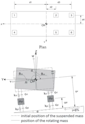
Thus, it can be concluded that the vehicle of class 3C is the most com-mon acom-mong heavy vehicles. This vehicle has been used in this work. As discussed previously, this work considered the nine-degree-of-freedom vehicle proposed by Moroz [14]: bounce of the suspended and non-suspended masses, and rotations around the longitudinal axis (roll) and transverse axis (pitch). The parameters used are
Table 1
Car mechanical and dynamic parameters
Parameter Value Unit
Vehicle suspended mass – mv 20.60 t Inertia moment of mass in roll – Ixx 15.00 t.m² Inertia moment of mass in pitch – Iyy 65.00 t.m² Front tire mass (non–suspended mass) – mpd 0.32 t t
Rear tire mass (non–suspended mass) – mpt 0.53 t t Front suspension system stiffness – kvd 432.00 kN/m
Rear suspension system stiffness – kvt 585.00 kN/m Front tire stiffness – kpd 840.00 kN/m Rear tire stiffness – kpt 1680 kN/m Front suspension system damping – cvd 3.00 kNs/m
Rear suspension system damping – cvt 6.00 kNs/m Front tire damping – cpd 1.00 kNs/m Rear tire damping – cpt 1.00 kNs/m
Distance d1 4.00 m
Distance d2 0.80 m
Distance d3 2.00 m
the same as those adopted by Santos [1] and Moroz [14], and are presented in table 1. Figure 1 shows the vehicle model used. The vehicle will be modelled considering the local axes v and w, in other words, the displacements of the vehicle (uv) and the tires (up,i) are
per-pendicular to the deck surface. Therefore, the vehicle interaction forces should be decomposed according to the super elevation so, only then, the interaction forces can be applied in the uniilar model of the bridge.
Given that the bridge is curved, an additional horizontal force is applied to the model: the centrifugal force. The centrifugal force can be added to the interaction forces from the dynamic analysis of the vehicle, as the vehicle has only vertical damp-ers and the lateral stifness of the tires are neglected. All these forces produce a moving load that travels along the bridge at a constant velocity.
Once the centrifugal force (Fc) is applied to the centre of mass of the suspended mass, it is necessary to know the height of the centre of mass with respect to the pavement, in order to obtain the associated transport moment. This height was found in Ejzenberg [19], which considers a distance of 2.16m for heavy trucks loaded. This distance was adopted in this work.
2.2 Structural modelling
For the study to be carried out in the later chapters, a bridge of the 900 branch of the Anhanguera complex will be analysed. The bridge has four curved spans (100m, 125m, 125m, 100m) and two straight 40m spans, as shown in igure 2. The radius of curvature in plan is constant and equal to 234.5m.
The structure is made of concrete, with box girder section of vari-able height in the curved stretches, it being higher in the region of the supports. After the curved sections there is a joint in the P4 column, which separates them from the two straight spans. These latter ones have cross section with constant height until the en-counter E2.
In the model, the properties of all sections were considered, ac-cording to the height variation shown. Figure 3 shows the prop-erties and dimensions of the sections of the support (a) and the middle of the span (b) of the curved section. For the straight spans the section is the same as in igure 3 (b).
The super elevation of the bridge varies from 2% to 6%, as shown in igure 4. For purposes of study, it was used only the maximum super elevation of 6%. In the P2 and P3 columns the superstruc-ture has an eccentricity of 90 cm in relation to the column. In col-umn P4 this eccentricity increases to 92.5cm.
It was considered a linear model for concrete, with compressive strength equivalent to 50 MPa for superstructure, 40 MPa for me-so-structure and 25 MPa for infra-structure.
The modelling of the analysed structure was done in the software ADINA - Automatic Dynamic Incremental Nonlinear Analysis [17]. The superstructure, columns and stakes were modelled with 3D bar elements, with properties equivalent to the respective sections. The blocks were modelled with shell elements, with thickness
Figure 1
Vehicle model
Figure 2
equivalent to the height of the blocks, since they have less compu-tational cost than solid elements and well represent the rigidity of the blocks. For the purpose of evaluating the displacements of the super-structure, it was considered suicient to model the stakes to a depth of 2m from the bottom of the block.
The supporting devices were modelled using bars, with the cor -responding degrees of freedom at their end. Rigid links were used to connect the support devices to the super-structure and to the columns. To simulate the super elevation of the bridge, given by the slope of the box girder section, the local systems of the 3D bars that model the superstructure were rotated. Figure 7 shows the ‘uniilar’ model of the bridge.
2.3 Pavement roughness proile
A proile of random irregularities can be described mathematically by means of spectral density functions, obtained experimental-ly. The roughness spectrum of the pavement adopted in this
work was calibrated by Honda [18], it being expressed by eq. 1.
(1)
where
α
depends on the state of conservation of the pavement, classiied in ive categories, according to the International Organi-zation for StandardiOrgani-zation (ISO); β is the exponent that depends on the material the pavement is made of, equal to 2.03 for asphalt pavements and 1.85 for concrete pavements; ωk is the wave fre-quency, deined as the inverse of the wavelength.According to Rossigali [16], among the various standardized scales that can be adopted as a measure of pavement irregularity, a widely used worldwide reference to denote pavement quality as a function of the roughness rate is the International Roughness Index (IRI). The correlation between ISO standards and the clas -siication scale adopted by DNIT as a function of IRI is presented in table 2.
Figure 3
Dimensions and properties of the cross-sections: (a) at the support (b) at the middle of the span (drawing
supplied by EGT Engenharia)
B
B
Figure 4
Cross-sections on pillars: (a) P1 (b) P2 e P3 (c) P4 (d) P5 (drawing supplied by EGT Engenharia)
B
B
B
B
A
C
B
D
Table 2
Correlation between the classifications adopted in Brazil (IRI) and by ISO
Pavement condition α(x10 -6m2/(m/ciclo) ) IRI (m/km)
The roughness proiles were generated from eq. (1) as a series of cosines (eq. 2) (Santos [1]):
(2)
where uir(x) is the random roughness of the pavement; αk is the roughness amplitude; ωk is the roughness frequency in cycles per meter; φk is the random phase angle deined in the interval [0.2π];
x is the position along the bridge axis and N is the total number of
terms in the series.
The amplitude αk is expressed by eq. (3):
(3)
Yang and Lin [20] deine the frequency increase by Δω=(ωmax -ωmin)/N, where ωmax and ωmin are the frequencies of maximum and minimum roughness admitted in the response.
According to Campos [21], the wavelength of the roughness should be between 0.5m and 50m. The waves with dimensions outside these ranges are evaluated as macro-texture, micro-texture and mega-texture, not to be considered as pavement irregularities. The roughness proile was obtained for an IRI of 4.10 m/km, which is classiied as poor-quality pavement. Figure 5 shows the irregu-larity proile adopted.
2.4 Application of the contact forces
on the structural model
The tires iteration eforts are statically condensed in the centre of mass of the vehicle, in order to obtain the vehicle reduced model. Thus, the loading model is reduced to three forces: vertical force (fwk), due to the bounce movement; transverse moment (mvk), due to the pitch movement; and longitudinal moment (mxk), due to the roll movement.
The interaction forces, due to the excitation of the vehicle, con-densed statically in its centre of mass, are then applied to the bridge ‘uniilar’ model. Of course, static loads due to vehicle weight
(P) and centrifugal force (Fc) should be added to the interaction
eforts. The vehicle is positioned eccentrically with respect to the axis of the bridge, considering the range of its furthest distance, in order to maximize the longitudinal moment (see igure 6a). The forces are then transported to the centre of mass of the cross sec-tion, generating a longitudinal moment equal to:
(4)
where h is the height of the pavement with respect to the centre of
the suspended mass, adopted equal to 2.16m, l is the eccentricity
of the vehicle in relation to the axis of the bridge, equal to 3.15m, and ys is the distance to the centre of mass of the structure,
vari-able for each cross section.
After calculating the longitudinal moment, the loads are applied to the bridge axis remembering that the interaction forces fwk and mvk must be decomposed according to the super elevation, to take from the vehicle axes w and v to the Z and Y axes of the ‘uniilar’ model (see igure 6b).
Note that the decomposition of the moment mvk generates a vertical
moment Mzk which, although small, is considered in the analysis.
Therefore, the vertical force Fzk in the global direction of the bridge
is shown in eq. 5:
(5)
The horizontal force from the decomposition of the interaction force must be added to the centrifugal inertia force, resulting in the total horizontal force Fyk to be applied in the bridge model (eq. 6).
(6)
The moment mvk must also be decomposed at a moment in the Y
direction and a moment in the Z direction (eq. 7).
(7)
It was considered that the applied moment Mykis equal to the
Figure 5
decomposed moment of interaction myk plus the moment due to the distribution of the vehicle’s own weight (eq. 8).
(8)
where Pi is the force that the wheel i exerts on the structure due to
the dead weight of the vehicle.
These forces are applied to the ‘uniilar’ bridge model, divided into three-dimensional beam elements, so that at each node k of the discretized bridge the ive reduced forces are speciied, i.e., verti-cal force (Fzk), transverse moment (Myk), longitudinal moment (Mxk), vertical moment (Mzk) and horizontal force (Fyk), see igure 7. Thus,
at the instant the vehicle is on node k, the ive reduced forces are
speciied and, for the other instants, these values are null, because the centre of mass of the vehicle is on other nodes.
3. Results and discussions
First of all, the modal analyses of the bridge and the vehicle, whose frequencies are found in table 3, were performed. From the irst two vibration modes of the bridge, the Rayleigh coeicients for 2.5% modal damping ξ were calibrated.
The bridge has very low frequencies, as seen in table 3. In this way, the higher the speed, the closer to the frequency of the bridge will be the loading of the vehicle. Thus, the study was carried out for the maximum speed for the traic conditions in the bridge of 80 km/h, as well as for speeds of 60km/h and 40km/h.
Firstly, the eforts of the vehicle-pavement interaction were ob-tained, under the initially adopted hypothesis of rigid deck. These eforts were decomposed according to the super elevation of the bridge, also considering the moments of transportation to the cen -tre of mass of the section of the bridge.
With the applied eforts in the model of the bridge the dynamic anal-ysis was carried out, resulting in temporal displacement functions for each node. As the applied forces were obtained considering rigid deck, they need to be adjusted, since the bridge has displace-ments when the vehicle travels along the bridge. This adjustment is performed through the iterative process described below:
Figure 6
(a) Positioning of the vehicle to calculate the forces. (b) Decomposition of the forces, according
to super elevation
B
B
A
B
Figure 7
1st Step: From the hypothesis of rigid deck and undeformed
struc-ture, for each instant t, the pavement roughness ur(xi) is applied to
each wheel i of position xi =x-d, x being the position of the centre
of mass (CM) of the vehicle at time t (x=V.t) and d the longitudinal
distance from the CM to the tire (see igure 8). By the dynamic analysis of the vehicle, the contact forces for each wheel f1(t) to
f6(t) are obtained.
2nd Step: Reduction of the forces into the centre of the suspended
mass for application in the ‘uniilar’ structural model.
Note that when the CM is at the beginning of the bridge (x=0) only
the irst wheel axle is on the bridge and is inluenced by the ir-regularity. The other axes, which would be outside the bridge, de-spite being considered because of the reduction of the forces in the vehicle centre of mass, are not subjected to any irregularity, and, therefore, would not inluence the dynamic response.
3rd Step: Application of the forces on the model of the bridge. 4th Step: Evaluation of the structural displacement, namely the
ver-tical translation (uzk,j(t)), longitudinal rotation (θxk, j(t)) and
transver-sal rotation θyk, j(t), for each node k, at the time t in which the vehicle
centre of mass (CM) is on it.
It is known that a displacement should be extracted for each wheel. However, due to the application of the reduced eforts, in this meth-odology a simpliication was adopted, obtaining only the displace-ments and rotations for the centre of mass of the vehicle. The
re-spective displacements for each wheel can be found by multiplying the longitudinal and transverse rotations by the corresponding dis-tances from the centre of mass to each wheel, adding these par-cels to the vertical displacements, as will be seen in the next step.
5th Step: The displacements obtained in the irst iteration j=1 are
added to the roughness of the pavement ur(xi) considered in the
irst step, for each wheel i and for each time t, in order to obtain an
“equivalent irregularity” function, considering the efects of struc-tural displacements distinctly on each tire line (see equation 9).
Table 3
Bridge and vehicle natural frequencies
Modes Bridge frequencies
(Hz) Bridge mode
Vehicle frequency
(Hz) Car mode
1 0,47 Vertical bending 1,68 Bounce of the suspended mass
2 0,59
Torsion with longitudinal displacement
2,15 Roll of the suspended mass
3 0,62 Lateral bending of
the straight span 2,23
Pitch of the suspended mass 4 0,69 Vertical bending 10,06 Roll of the
non-suspended mass 5 0,89 Lateral bending
with torsion 10,14
Pitch of the non-suspended mass 6 0,92 Lateral bending
with torsion 10,40
Roll of the non-suspended mass
Figure 8
Application of the irregularity on the vehicle model
Figure 9
Figure 10
Figure 11
Figure 12
(9)
where l is the distance from the bridge axis to the vehicle axis.
6th Step: New contact forces are obtained by the dynamic analysis
of the vehicle, under the support excitation provided by the “equiv-alent irregularity” of the 3rd step.
7th Step: After the new contact forces are obtained, the responses
of the interaction forces in the frequency domain are determined by applying the Fourier transform to each iteration.
8th Step: The deviations between the result in the frequency domain
of iteration i and iteration i-1 are calculated using the SRSS criterion
- Square Root of the Sum of Squares for the maximum amplitudes.
9th Step: If the deviation between two consecutive iterations is less than
Figure 13
1%, then it is considered that convergence has been obtained and the inal model analysis is performed. If not, steps 2 through 6 should be repeated until convergence of the interaction forces are obtained. Figure 9 shows a lowchart with the proposed methodology. In this study, only three iterations were necessary to obtain the conver -gence of the interaction forces, except for the speed of 60 km/h for which
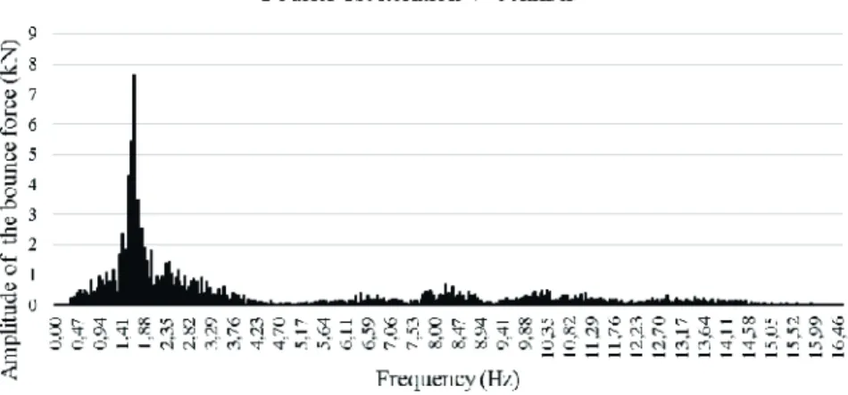
only two iterations would be suicient. Figures 10 to 12 show the com-parison of the forces applied to the bridge for the irst and third iterations. It was obtained the Fourier transform of the interaction force
Fz, referring to the bounce motion, for each iteration, evaluating
the deviation between the result of the iteration i and the itera -tion i-1, using the SRSS criterion - Square Root of the Sum of
Figure 14
Squares for the maximum amplitudes, as indicated in eq. 10:
(10)
where n is the number of frequencies considered for the
calcula-tion of the amplitudes
Figures 13 to 15 show the Fourier analyses for each interaction. Note that, for all iterations, the highest amplitude peak has a fre-quency corresponding to 1.67 Hz, very close to 1.68 Hz of the irst bounce mode of the vehicle’s suspended mass. It is also noticed
Figure 15
that there is an increase in the amplitudes near the frequencies of 8 to 10 Hz, which are close to the vibration modes of the non-sus-pended masses of the vehicle, but with much smaller amplitudes. Table 4 shows the diferences found between the iterations. From the static point of view, one would expect that the rigid deck situation would correspond to larger contact forces and then, with the correction of the displacements, the lexibilization of the deck would decrease the inter-action forces. However, this didn’t occur in a general way in the dynamic analysis. Depending on the frequency that is excited, the lexibilization of the deck can increase or decrease the interaction forces. As seen in Table 4, for the velocities of 40km/h and 60km/h, the interaction forces increased from the irst to the last iteration, whereas for the velocity of 80 km/h the interaction forces were reduced.
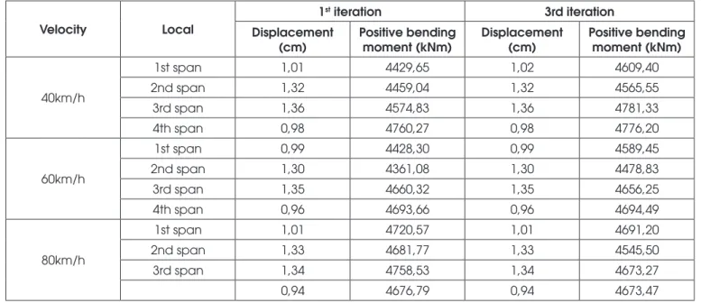
Table 5 presents the displacements and positive bending moments for the 1st and 3rd iterations for the speeds of 80km/h, 60km/h and
40km/h. A good convergence is observed, with small diference of the results of bending moments, and the structural displacements practically did not change.
For the purpose of illustration, igures 16 and 17 present the history of displacements and bending moments in the four curved spans, where one can observe the proximity of the answers between the 1st and 3rd iterations.
4. Conclusions
The most important product of this work is the proposition of a sim-pliied methodology for the dynamic analysis of curved bridges, in which the separation of bridge and vehicle models is postulated, and these are coupled only by the interaction forces. For the deter-mination of these forces it is considered that the vehicle is initially on a rigid deck and, later, this hypothesis is corrected, through an iterative process. This methodology is both simple and accessible to structural engineers, using a commercially available inite ele-ment program. Thus, designers will be increasingly able to perform dynamic analyses on curved bridges, simultaneously considering the efect of moving loads constituted by centrifugal forces and vehicle-pavement interaction forces, and using more realistic mod-els that consider the data referring to the actual traic in the road networks, as well as the state of conservation of the pavements. In the case study addressed herewith, no more than three itera-tions were necessary to obtain convergence of the interaction forces. It was observed that, depending on the frequency being excited, the interaction forces may increase or decrease with the lexibility correction, diferently to what is expected under purely static reasoning, according to which the more rigid the deck, the larger the load it would absorb.
It was also observed a good convergence in the dynamic respons-es of the bridge, with small diference of the bending moments
Table 4
Difference between the iterations using
the SRSS method
Velocity Iteration Deviation (%)
80 1-2 -3,60 2-3 -0,10 1-3 -3,70 60 1-2 0,34 2-3 -0,20 1-3 0,14 40 1-2 8,5 2-3 -0,03 1-3 8,47
Table 5
Displacements and positive bending moments – 1
stand 3
rditeration
Velocity Local
1st iteration 3rd iteration
Displacement (cm) Positive bending moment (kNm) Displacement (cm) Positive bending moment (kNm) 40km/h
1st span 1,01 4429,65 1,02 4609,40 2nd span 1,32 4459,04 1,32 4565,55 3rd span 1,36 4574,83 1,36 4781,33 4th span 0,98 4760,27 0,98 4776,20
60km/h
1st span 0,99 4428,30 0,99 4589,45 2nd span 1,30 4361,08 1,30 4478,83 3rd span 1,35 4660,32 1,35 4656,25 4th span 0,96 4693,66 0,96 4694,49
80km/h
Figure 16
Figure 17
Comparison of the positive bending moments My for the 1
stand 3
rditeration – V=80km/h
between the irst and third iteration, and the structural displace-ments practically did not change.
It is worth emphasizing that the results presented here are com-pletely dependent of the structural typology and its dynamic char-acteristics, and may present considerable diferences if some of these factors are altered. However, the proposed methodology
and the iterative procedure through simple adaptations remain an adequate means to evaluate the structural dynamic response.
5. Acknowledgments
de-sign data of the Anhanguera bridge, object of study of this work. The second author acknowledges a grant from CNPq (3-2757/2013-9).
6. References
[1] SANTOS, E. F. Análise e redução de vibração em pontes rodoviárias. Doctoral Dissertation (in Portuguese), COPPE/ UFRJ, Rio de Janeiro, RJ, Brasil. 2007.
[2] ALMEIDA, R. S. Análise de vibrações em pontes rodoviárias induzidas pelo tráfego de veículos sobre pavimentos irregu-lares. Master Thesis (in Portuguese), UERJ, Rio de Janeiro, RJ, Brasil. 2006.
[3] WILLIS, R. Appendix to the Report of the Commissioners Appointed to Inquire into the Application of Iron to Railway Structures. Stationary Oice, London. 1849.
[4] STOKES, G. Discussion of a diferential equation relating to the breaking of railway bridges, Trans. Cambridge Philo-sophic Soc, v8. 1849.
[5] MELO, E.S Interação dinâmica veículo-estrutura em pequenas pontes rodoviárias. Master Thesis (in Portu-guese), UERJ, Rio de Janeiro, RJ, Brasil. 2007.
[6] INGLIS, C.E. A Mathematical Treatise on Vibrations in Rail-way Bridges. Cambridge Univ. Press, London, 1934 [7] TIMOSHENKO, S., Vibration Problems in Engineering. 3rd
Edition, D. Van. Nostrand. 1964.
[8] HUANG, T., VELETSOS, A.S. Analyses of Dynamic Response of Highway Bridges. ASCE, J. Mech, Div., 1970. Vol. 96. [9] BRUCH, Y.A. Análise Dinâmica de Placas Retangulares
pelo Método dos Elementos Finitos. Master Thesis (in Portu-guese), COPPE/UFRJ. RJ, Brasil, 1973
[10] CARNEIRO, R.J.F.M. Análise de Pontes Rodoviárias sob Ação de Cargas Móveis. Master Thesis (in Portuguese), PUC-Rio, Rio de Janeiro, RJ, Brasil. 1986.
[11] FERREIRA, K.I.I. Avaliação do Critério para Cálculo dos Efeitos de Cargas Móveis em Pontes Rodoviárias. Master Thesis (in Portuguese), PUC-Rio, RJ, Brasil. 1991.
[12] CHANG, D., LEE, H., Impact Factors for Simple-Span Highway Girder Bridges. Journal of Structural Engineering, ASCE, v.120, n.3, pp704-715.
[13] NOWAK, A.S. Load Model for Bridge Design Code. Cana-dian Journal of Civil Engineering., v21, pp.36-49. 1994. [14] MOROZ, F. V. Uma metodologia para análise da inluência
do tráfego de veículos pesados na resposta dinâmica de pontes rodoviárias. Master Thesis (in Portuguese), EPUSP, São Paulo, SP, Brasil. 2009.
[15] ROSSIGALI, C. E. Estudos probabilísticos para modelos de cargas móveis em pontes rodoviárias no Brasil. Master Thesis (in Portuguese), COPPE/UFRJ, Rio de Janeiro, RJ, Brasil. 2006.
[16] __________. Atualização do modelo de cargas móveis para pontes rodoviárias de pequenos vão no Brasil. Doctoral Dissertation (in Portuguese), COPPE/UFRJ, Rio de Janeiro, RJ, Brasil. 2013.
[17] ADINA - Automatic Dynamic Incremental Nonlinear Analy-sis Software: version 9.0.1. Developed by ADINA R&D, Inc. Massachusetts, 2013. Available at: http://www.adina.com. Access in 06/02/2015.
[18] HONDA, H., KAJIKAWA, Y., KOBORI, T., Spectra of Road Surface Roughness on Bridges. Journal of the Structural Di-vision, ASCE, v108, ST9, pp 1956-1996, 1982
[19] EJZENBERG, S. Os veículos pesados e a segurança no projeto das curvas horizontais de rodovias e vias de transito rápido. Master Thesis (in Portuguese), EPUSP, São Paulo, SP, Brasil. 2009.
[20] YANG, Y, LIN, B. Vehicle-Bridge Interaction Analysis by Dynamic Condensation Method. Journal of Structural Engi-neering, ASCE, v121, pp 1636-1643, 1995.