A Work Project, presented as part of the requirements for the Award of a Masters Degree in Management from the Faculdade de Economia da Universidade Nova de Lisboa
Steel Futures and Company
Characteristics: Which
Companies use Steel
Futures?
Alexander Nikles (24790/2709)
A Project carried out on the Corporate Finance course,
with the supervision of:
Miguel Ferreira
04/01/2017
Steel Futures and Company Characteristics:
Which Companies use Steel Futures?
Abstract
My thesis examines the link between firm characteristics and the usage of steel futures working with annual data from 1,536 steel-related companies’ between 2003 and 2015. I use fixed effects regression with binary response to estimate a firm’s likelihood of using steel futures. The chance of using steel futures for firms with a high degree of steel exposure relative to less steel exposed ones, is significantly positively affected by firm size, leverage, debt structure, return on assets and investment grade.
1. Introduction
In 2008 the London Metal Exchange and Chicago Mercantile Exchange Group introduced future contracts for standardized steel products. For the first time, there has been an exchange-traded derivative for the world’s second largest commodity after crude oil (Morrison, 2011). Regardless of whether medium-sized steel processor, automotive industry or multinational steel producer, manufacturers and buyers are more or less strongly dependent on the steel price. Especially in China, world’s largest steel producing economy, steel futures have seen robust growth in the past years and “Shanghai Futures Exchange and Shanghai Steel Exchange Center each see hundreds of thousands of trades a day” (Day, 2011; see also Appendix 1).
Previous research conducted by Almeida et al. (2016) finds that steel futures partly substitute existing hedging instruments, i.e. purchase obligations. In the statistical analysis Almeida et al. (2016) include company characteristics as control variables. In doing so, he partly shed light on the question, whether, for instance, a firm’s leverage, firm size or R&D expenses may affect its hedging behavior. In particular, Almeida et al. (2016) find proof that a firm’s steel exposure positively affects the usage of steel futures. Intuitively this makes sense, since steel futures have been introduced to serve a certain audience, namely corporations, suffering from steel price volatility. In turn, the extent to which firms are affected by steel price volatility depends on a firm’s steel exposure, i.e. steel inputs and outputs.
Hence, in my thesis, I focus on highly steel-exposed firms and how their hedging behavior is affected by firm characteristics. More precisely, I seek to deepen the understanding whether and which company characteristics increase the likelihood that highly steel-exposed companies use steel futures to hedge their steel-related price risk. To do so, I use the analysis of Almeida et al. (2016) as a starting point to confirm the favoring effect of steel exposure on steel future usage (Main Effect). Then, I add interaction terms to test a manifold set of firm characteristics. The interpretation of interaction effects allows a detailed insight into the
interdependence between the introduction of steel futures, company characteristics and high steel exposure. In other words, interaction effects help to assess the precise effect of each of the objects of interest. For instance, are above-average-sized firms with a high degree of steel exposure generally more likely to hedge after 2008 than above-average-sized firms with less steel exposure.
In my research, I find, that after the introduction of steel futures in 2008, the likelihood of using commodity derivatives increase more for highly steel exposed firms compared to less steel exposed firms. Furthermore, this main effect is stronger for ex ante (1) large, (2) highly levered and (3) profitable firms, which hold an (4) investment rating. To the best of my knowledge, the latter evidence exploiting the introduction of steel futures as a quasi-natural experiment is new to the literature.
The subsequent literature review aims to emphasize important theoretical considerations regarding risk and liquidity management and hedging and discusses previous empirical findings.
2. Literature Review and Hypothesis Development
Corporations and individuals aim to diminish the variability in their earnings. This is especially true for the steel business, which is strongly cyclical, driven by macro trends and challenged by technological advances (Rohini, 2004; also see Appendix 2). According to a survey conducted by Rawls and Smithson (1990), risk management is considered to be one of the most crucial activities in corporations’ financial departments. The relevance of the survey is confirmed by recent growth numbers for exchange-traded derivatives. According to Sundaram (2013), the trading volume of future contracts and options has grown by a compound annual growth rate of more than 11% from 1998 to 2011.
2.1. The Rationale of Hedging: Why do Firms hedge?
First, the existing literature emphasizes the impact of managers’ personal risk aversion and their inability to diversify their individual portfolio on their hedging behavior (Stulz, 1984). In accordance to Stulz (1984), the shareholders of the company usually hold a diversified investment portfolio, while the manager of a company is strongly dependent on the company’s results. The manager’s portfolio is barely diversified and characterized by his individual risk aversion. Hence, the manager aims to mitigate the company’s earnings variance in order to smoothen his own income variability. Another approach emphasizes the impact of the structure of corporate income taxes and bankruptcy costs (Smith and Stulz, 1985). Hedging activities may allow the company to optimize their capital structure. More precisely, hedging activities typically transfer the company’s risk outside the corporation, thus increasing the amount of debt the company can sustain. This increase in corporate leverage leads to tax savings since cost of external financing is tax deductible. In addition, Smith and Stulz (1985) point out, while bearing in mind that the company’s income tax function is convex, that it is desirable for companies to have less peaks and valleys in their earnings since the expected tax burden of a more volatile income is higher.
2.2. The Credit Rationing Model
Another research study published by Froot, Scharfstein and Stein (1993) points out, that a company inevitably increases its internal variability in terms of earnings and cash-flows by waiving hedging instruments. An increased variability immediately affects a company’s funding and investment behavior. For instance, a negative variation in cash flows will compel the company to increase their external financing in order to sustain the company’s desired level of investment. However, under some circumstances lenders may deny the additional credit due to market imperfections. This phenomenon is known as credit rationing. In order to avoid suffering from credit rationing, it may be valuable for companies to hedge.
Previous literature has uncovered various potential explanations for the occurrence of credit rationing. One of them is adverse selection, which leads to an outcome, where only the riskiest projects receive sufficient external financing due to the lenders’ focus on profit maximization (Stiglitz and Weiss (1981), Allen (1983) and Bester (1985)). Another approach to credit rationing has been published by Holmström and Tirole (1998) and rather focussesthe impact of moral hazard and agency costs on the supply of external financing.
In order to build a theoretical foundation for the empirical analysis, I now illustrate Tirole’s (2006) model for risk and liquidity management.
2.2.1. Single Period Fixed Investment Model
Following Tirole (2006), an entrepreneur seeks external financing in order to fund an investment, whose probability of success and return 𝑅" is uniformly distributed with 𝜏. Moreover, the chance of success of the investment depends on the effort undertaken by the entrepreneur, 𝜌% in the case of high effort and 𝜌& in the case of low effort. The size of external funds required equals the difference between the amount to be invested and the entrepreneur’s assets. In case of low effort, the entrepreneur enjoys a private benefit 𝐵. Hence, the loan agreement needs to be structured in a way, that allows the lender to remunerate himself for the capital expenditure, while offering the entrepreneur a sufficient incentive to omit misbehavior, i.e. low effort. Due to this, the entrepreneur has to participate in the success of the investment with share 𝑅(. A lender will only commit to an investment if:
𝑝*∗ 𝑅( ≥ 𝑝-∗ 𝑅(+ 𝐵 (1)
A borrower is deterred from misbehavior, if this inequality holds. The ability to assess the effort of the entrepreneur seems to be crucial to accomplish a loan agreement with aligned interests. In reality, the lender is unable to observe whether the entrepreneur misbehaves or not. Therefore, the entrepreneur must secure the loan with own assets. If the entrepreneur is not able to provide a minimum of liquid assets, i.e. cash, potential lenders will refuse to provide the
loan. Hence, the company is rationed in their ability to raise credit. In other words, credit rationing describes the situation where borrowers are unable to take out a loan, even if they are willing to bear the required interest (Tirole, 2006). Thus, one determinant of credit rationing is the availability of internal, liquid assets. Furthermore, apart from direct credit cost 𝐶", credit rationing is affected by the corresponding agency costs. The agency cost (or agency rent) equals the incentive (𝐶0), which needs to be granted to ensure the entrepreneur’s high effort. The higher the agency cost, the higher the probability of credit rationing. In order to be able to achieve a state without credit rationing, following condition needs to be fulfilled (Tirole, 2006):
(𝜌% − (𝑝&+ 𝜏)) ∗ 𝑅" > 𝐶"+ 𝐶0 (2)
The interpretation of equation 2 is intuitive. The expected return 𝑅" must exceed the sum of total direct credit cost 𝐶" plus incentive-related costs 𝐶0.
2.2.2. Intermediate Stage and Liquidity Shocks
In order to study the role of risk management, Tirole (2006) extends the basic model with an intermediate state: The entrepreneur may experience a liquidity shock in the intermediate stage, which deters the entrepreneur from entering into new promising investment opportunities, serve reinvestment needs or maintain their daily businesses.
In comparison with the basic, two-stage model, the three-stage model with an intermediate stage is complemented by an intermediate income (r) and a reinvestment need (𝜌). However, to avoid moral hazard in the intermediate stage, the intermediate compensation r is exchanged by a higher compensation in the final stage. Again, in this setting the maximum reinvestment amount granted by the lenders depends on the moral hazard induced by the entrepreneur. If the costs of a rescue, contingent on the incentives for the entrepreneur, exceed the expected payoff, depending on the entrepreneur’s high or low effort, lenders will refuse to reinvest. Additionally, the outcome of the reinvestment negotiation is strongly affected by the value of company-owned assets in the intermediate stage since they determine the available amount of liquidation.
The higher the value of the assets that can rapidly be converted into cash (or cash itself), the higher the pledgeable income, that in turn determines the amount granted by the lenders (Tirole, 2006). Going back to the initial classification of solvent and illiquid companies, one may infer a general statement concerning liquidity management in a three-stage model: Both companies, solvent and illiquid, must plan their liquidity needs in advance. For solvent firms this happens through the determination of a tailored debt structure and an accurate payout ratio. For illiquid firms at least by securing their credit lines in accordance to the firm value. In other words, managing liquidity either means sustaining a sufficient cash buffer or using financial instruments to mitigate the effect of adverse shocks on the company’s income and investment portfolio.
2.3. Empirical Findings
As initially stated, risk management is considered to be one of the most crucial corporate financial tasks. Recently, risk management has been innovating a lot and novel hedging instruments have emerged. This setting allows us to examine situations, where novel hedging instruments have been introduced and some of the companies start to deploy these instruments, while others do not. The following section has two major objectives. First, it outlines previous statistical evidence describing the effect of hedging activities on company characteristics, such as market valuations. Second, it discusses previous research focusing on the extent to which certain company characteristics favor the usage of hedging instruments.
2.3.1. Hedging influences Firm Characteristics
Ongoing innovation allowed hedging instruments to penetrate more and more industries and corporations. Weather hedges are one of the most recent innovations in this area. The effect of the introduction of weather hedges on firm value has been analyzed by Péréz-Gonzalez and Yun (2013). This mechanism allows company to decrease their dependence on external weather conditions. According to the authors, the introduction of weather hedges was followed by three
effects. First, a significant increase in the market valuations of hedging companies. Second, an enlarged investment volume, which is in line with the previously presented model that externalization of risk increases a company’s credit capacity (Smith and Stulz, 1985; Tirole, 2006). Third, companies took advantage of their expanded credit capacity and increased their leverage. A study conducted by Carter et al. (2006) obtained evidence, that fuel hedges positively affect airline companies’ market values. It is pointed out, that this increase in firm value is primarily achieved by reducing the underinvestment costs. Agency costs of underinvestment occur, when shareholders reject to invest in low-risk investments to prevent a shift in wealth in favor of the companies’ debtholders (Myers, 1977). On the contrary, a study conducted by Jin et. al (2006) did not find sufficient evidence, that hedging activities of oil and gas producers exert a significant influence on the companies’ market valuations.
Gilje and Taillard (2015) point in another direction and provide an insight into corporate hedging activities of oil producers. In their research on the effect of external risk shocks they present empirical evidence, that firms hedge because they aim to diminish the likelihood of financial distress and decrease the risk of underinvestment, which in turn affects firm value. This finding is in line with the theoretical explanations by Smith and Stulz (1985).
Another empirical study that supports the previously presented theoretical approach by Froot et al. (1993) can be found in a research study on highway construction in the U.S, where procurement costs had been decreased significantly after relieving construction companies from oil price risk (Howell, 2015). Howell (2015) finds, that those companies are typically facing low cash flow and hence limited investment ability, when their exposure to oil price risk is the greatest.
2.3.2. Company Characteristics affect the Probability of Hedging
In line with the theoretical model by Tirole (2006), it seems straightforward to assume, that some companies are more likely to hedge than others due to structural differences. Previous
research has confirmed this intuition. A study conducted by Gay and Nam (1998) points out, that companies with promising growth opportunities and low cash are more likely to be engaged in hedging. They further outline, that this positive relationship is to some extent driven by the companies’ objective to avoid underinvestment. In line with these findings, Carter et al. (2006) points out, that airline companies with promising investment opportunities tend to hedge more. In accordance with those findings, Nance, Smith and Smithson (1993) provide evidence that hedging is favored by the growth opportunities in a company’s investment portfolio. Moreover, Nance, Smith and Smithson (1993) present statistical evidence, that firm size is positively associated with hedging. However, one need to consider the findings by Byoun (2007) stating, that large firms also show significantly lower indebtedness, thus a lower chance of financial distress. Gézcy et al. (1997) also find a significantly positive relationship of growth opportunities, measured by long-term debt times market-to-book value, firm size and hedging while underscoring the impact of financial limitations. An insightful study conducted by Adam (2009) finds significant, positive correlation between a mining company’s capital expenditures and hedging. This supports previous arguments, that companies with promising investments at hand, will engage in hedging in order to mitigate volatility in their cash-flows. However, other studies, such as Graham and Rogers (2002), reject the hypothesis, that a company’s prospective growth opportunities affect their hedging behavior significantly. After providing an insight into existing research on risk management and hedging, the following section derives the hypotheses to be tested and depicts the methodological approach.
2.4. Hypotheses Development
Both the credit rationing model by Tirole (2006) and previous empirical findings suggest a relationship between company characteristics and corporate hedging behavior. As a starting point, it seems reasonable to expect a positive relationship between hedging and growth opportunities. Companies expecting to expand their business in the near future, will usually
also expect to take out a loan or seek alternative external financing. In turn, an increased debt burden requires financial planning to be able to bear the long-term borrowing costs. Furthermore, a company’s hedging behavior may also be affected by its individual credit default risk, i.e. the existence of an investment grade, and their debt structure, as both characteristics determine a firm’s credit costs. Finally, hedging, in particular exchange-traded derivatives, require knowledge and induce costs, i.e. transaction costs. Hence, exchange traded-derivative may primarily be used by large corporations. Accordingly, I define six hypotheses.
Treatment-Related Hypotheses 1
(1a) Highly steel-exposed companies are significantly more likely to use steel futures after
2008.
Firm-Characteristics-Related Hypotheses 2a – 2e
(2a) The probability a highly steel-exposed firm is hedging after 2008 is positively correlated with the firm’s growth opportunities, measured by Tobin’s Q.
(2b) The probability a highly steel-exposed firm is hedging after 2008 is negatively related to the firm’s cash holdings.
(2c) The probability a highly steel-exposed firm is hedging after 2008 is significantly correlated with its total assets (firm size).
(2d) The probability a highly steel-exposed firm is hedging after 2008 is determined by a company’s leverage and its structure. A high leverage with a proportionally high share of long-term debt increases the likelihood of hedging.
(2e) The probability a highly steel-exposed firm is hedging after 2008 is negatively correlated with the existence of an Investment Rating.
3. Data
In the following I illustrate the data collection and assembling process. Furthermore, some challenges that occurred during the collection are described.
3.1. A panel dataset
First, I collected 10-K and 20-F annual financial reports for 1,536 companies identified by their Central Index Keys (CIKs) from 2003 to 2015 and stored by the US Security Exchange Commission (SEC). The list of 1,536 companies was retrieved by analyzing the Bureau of Economic Analysis (BEA) input-output table in order to pick all companies having an input share larger than 1% from steel producing industries and companies, which belong to those steel producing industries itself. The limitation to firms having a steel exposure higher than 1% was made in order to facilitate parsing and limit the sample for practical reasons.
A set of 11,488 filings was collected and parsed for an extensive list of keywords (see Appendix 3), which largely follows Almeida et al. (2016). Our parsing result ends up to be a list of 11,488 lines consisting of a column for each search term and a binary variable, which is set to 1 in case one of the keywords is found and to 0 otherwise. This data is cleaned and merged in various dimensions. For instance, some firms had 10-K filings, but after a certain point in time there have been no records in Compustat anymore. Moreover, I exclude observations with negative assets, sales or capex. Companies, which at least reported one of the keywords in the respective filing, are expected to be hedging against steel price volatility in the respective year. In a second step, accounting data are retrieved from Compustat. For this purpose, the list of CIKs was matched with their counterpart in Compustat, the Global Company Key (GVKEY). Following, I draw data on returns and security prices from the Center for Research in Security Prices (CRSP) by matching GVKEYS and CRSP’s Permanent Company Identifier (PERMCO).
3.2. Data-related Assumptions and Limitations
A main limitation, which is caused by parsing the annual reports for a rather generic list of keywords diminishes the precision of the parsing results. In this context, one should consider the following. The parsing results neither enable us to identify the specific hedging instrument used by the company nor do they specify the magnitude of hedging efforts. However, the
chosen, less complicated method facilitates the creation of a much larger sample while still allowing to assess the impact of the introduction of steel futures. Furthermore, the parsing results may identify some companies as being commodity hedger while those companies actually do not engage in hedging. This phenomenon is due to the “syntax sensitivity” of textual analysis. For instance, some companies may describe their risk management as follows: “Our company does not engage in hedging, such as commodity futures or options”. I checked a selection of reports manually and concluded that this issue is not a serious constraint for the statistical analysis. Thus, I assume that each company that reports one of the keywords in their annual report is using hedging instruments. Moreover, as I seek to find a treatment effect of the introduction of steel futures in 2008, the assumption holds, that the effect of firms being falsely considered as commodity hedgers would similarly distort both pre- and post-treatment companies. Hence, it seems reasonable to exclude this issue from our analysis. Furthermore, it is important to bear in mind, that the 10-K filings merely disclose information regarding the usage of hedging instrument. Usually, these reports do not specify whether steel futures are used or not. However, thanks to the experimental setting described in the following section, the firm’s disclosure is not necessary to assess which companies are actually using those novels contracts.
4. Methodology and Variables
Again, the objective of this research is to identify company characteristics, which significantly affect the probability of being a steel future user while considering a company’s high steel exposure and the treatment in 2008. As described in detail in the previous section, I use a panel data set consisting of 1,536 steel-related companies between 2003 and 2015. The introduction of steel futures in 2008 can be understood as an experimental setting as before 2008 all companies from the sample merely had access to a limited selection of hedging tools, such as purchase obligations. From 2008 onwards their toolbox of hedging instruments was
complemented with future contracts on several steel products. As stated in the introduction, steel futures have been introduced for a certain audience. Usually, firms which are strongly affected by steel price volatility. Again, this was also the motivation to limit the sample to firms with at least 1% steel-exposure. Thus, my approach is incremental. First, I seek to prove the positive effect of high steel exposure on the usage of steel futures after 2008. This is shown in a similar way by Almeida et al. (2016). Second, within the group ofhighly steel-exposed firms, and this is novel, I seek to assess the effect of certain firm characteristics by using triple-interaction terms. To pursue this two-stage approach, I use a Difference-in-Differences Estimation (Woolridge, 2009). We use a set of control and treatment variables, which are depicted in table 1.
Table 1. Variable Definition and Computation
According to Woolridge (2009), this approach is particularly advantageous for assessing the effect of a single event, treatment or policy. The introduction of steel futures in 2008 is such
a treatment. All firms showing a steel exposure larger than 1% but less or equal to 10% are assigned to the control group. All firms showing a steel exposure above 10% are assigned to the treatment group, because the 10% reflect the 75% percentile of the steel exposure in the sample (see Appendix 4). As such, it includes all firms with are particularly affected by steel price volatility. However, it is important to bear in mind, that the exact value of the chosen threshold should not affect the interpretation of my results, since its sole purpose is to distinguish less steel-exposed firms from more steel-exposed firms. Our treatment effect, as said, is the introduction of steel futures in 2008. Regarding the econometric model, our dependent variable Commodity Hedger is binary as it will either be 1 if the company is hedging or 0 otherwise.
Woolridge (2009) specifies two main approaches for binary response variables: Linear Probability Model and Index Models. The Linear Probability Model largely offers the main benefits of a normal linear regression model, in particular its good interpretability. It constitutes as follows:
𝑃 𝑦 = 1 𝑥 = 𝛽; + 𝛽"𝑥"+. . . +𝛽=𝑥= (3)
An incremental increase in an explanatory variable (all else equal) indicates the change in the probability of being a commodity hedger (𝑦 = 1). The direction and magnitude of each explanatory variable is determined by 𝛽>. For example, if 𝛽> = 0.01 a one unit increase in 𝑥>
will increase the chance that y becomes 1 by 1%. However, the Linear Probability Model comes with disadvantages, such as constant marginal effects and predicted outcomes beyond one and below zero (Woolridge, 2009). An alternative approach, Almeida et al. (2016) followed, is the usage of a non-linear index model, i.e. probit or logit. Index models for binary response variable are sometimes advantageous since they naturally limit the dependent variable Y between 0 and 1 and do not have constant marginal effects (Woolridge, 2009). However, my sample consists of panel data and I control for year and firm fixed effects. I use fixed effects
regression due to the fact that I seek to elaborate the effect of a set of company characteristics on the likelihood of being commodity hedger over the period from “pre 2008” to “post 2008” and some variables used in the regression do not change over time (Allison, 2005). In my case, the sample includes both time-invariant explanatory variables, for instance Steel Exposure and all variables with the ending “_2007”, and firm-invariant variables, such as the Steel Futures Available dummy. Fixed effects regression addresses these issues but brings increased complexity especially regarding the usage of interaction terms. In my case, the interaction terms are the main interest of the analysis since they clearly indicate how certain company characteristics have affected steel-exposed firms after 2008, i.e. which companies actually use steel futures. According to Ai and Norton (2003) the integration and interpretation of interaction terms in logit and probit in terms of marginal effects can be misleading. This issue is further specified by Karaca-Mandic, Norton and Dowd (2012) concerning interaction effects in non-linear models with fixed effects. According to Karaca-Mandic, Norton and Dowd (2012), interaction effects in index models, such as logit and probit, are problematic due to the omitted constant and only applicable under strong assumption, i.e. fixed effects are zero.
All in short, due to the downside of non-linear models in terms of interaction effects, I am using a fixed effects linear probability model maximizing the within-R2 of the estimate.
In order to retrieve robust standard errors, they are clustered by industry#year. Furthermore, in the interaction terms, I use “de-meaned” company characteristics. More precisely, I compute the mean value of each company characteristic across the sample at the end of 2007. Afterwards, this mean value is subtracted from each firm’s value of the corresponding characteristic. The result is a “de-meaned” value for each company characteristic and firm. This approach allows me to analyze, for instance, the effect of an above-average leverage on the probability of being commodity hedger for a highly steel-exposed firm.
5. Descriptive Statistics
As initially stated, I retrieve data from 2003 to 2015 on 1536 firms having a steel-exposure larger than 1%. I ended up with 8,292 firm years. I find that in 1,142 firm years (≈13.8%) our response variable “Commodity Hedger” equals one. Furthermore, we find that the average steel exposure across these 1536 firms is 6.7%. The 75% quintile equals roughly 10% (see Appendix 4). Due to this, as described before, in the regression, the dummy variable “High Steel Exposure” is set to one if the firm’s steel exposure exceeds 10%. The summary statistics concerning the previously defined variables are listed in appendices 5 and 6. Appendix 5 depicts the statistics for less steel-exposed firms, whereas table Appendix 6 depicts highly-steel exposed firms. Its particularly interesting to observe that firm characteristics for highly steel-exposed firms seem to be different from less steel-steel-exposed firms’ characteristics. For instance, less steel-exposed firms have a mean leverage of 15.4%, highly steel-exposed firms bear on average a leverage of 20.2%. Furthermore, the mean firm size for highly steel-exposed firms equals 6.63 (logarithmized assets total) and is larger than the mean firm size of less steel-exposed firms with 5.97. A similar observation can be made regarding long-term debt to assets ratio. The average long-term debt ratio for highly-steel exposed firms is 3.7 % pt. larger than for less steel-exposed firms.
To check for differences in treatment and control statistically, I performed a t-test on all control variables at the end of 2007. I find no statistical evidence, that any company characteristic is significantly different comparing highly or less steel-exposed firms (See Appendix 7).
6. Results
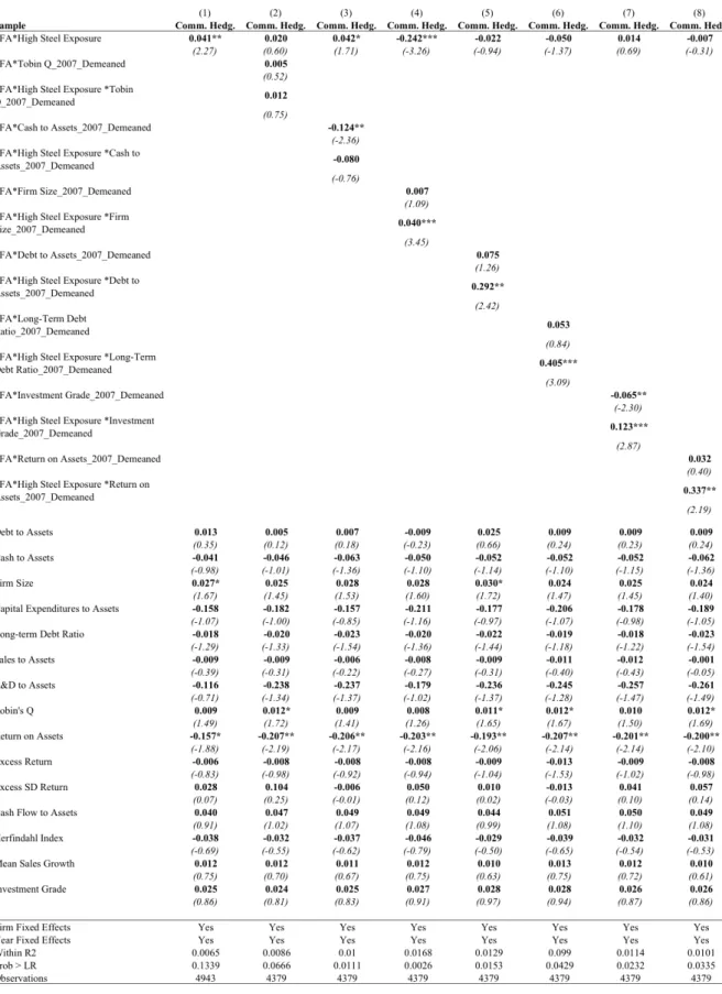
The results of a regression with binary response variable and both firm and year fixed effects is shown in table 3 on the following page. Column (1) reports the impact of the introduction of steel futures merely considering control variables and the interaction term High Steel
Exposure*Steel Futures Available as done by Almeida et al. (2016). The variable “Steel Futures Available” is omitted due to year fixed-effects, i.e. the variable is not time varying. I assume, that in the paper by Almeida et al. (2016) one year was omitted instead. Furthermore, one need to bear in mind the dummy High Steel Exposure indicates an exposure larger than 10% since all sample firms have a steel exposure > 1%.
Column (1) suggests that a high-steel exposure increases the hedging probability by 4.1% after 2008. Thus, we can confirm hypothesis 1a. Highly steel exposed firms are ceteris paribus (c.p.) more likely to be hedging after the introduction of steel futures in 2008. This insight underlines the finding of Almeida et al. (2016). Furthermore, Appendix 8 confirms the parallel trends assumptions. The parallel trends assumption suggests, that before the treatment the dependent variable y developed similar for the treatment and the control group (Friedman, 2013). Indeed, the curve is similar before, but diverges after 2008. More precisely, before 2008 the average likelihood of being a commodity hedger for less steel-exposed firms are 8,79% and 13,59% for highly steel-exposed firms. After 2008, the mean value constitutes as 13,41% for less steel exposed firms and 24,39% for highly steel-exposed firms. To sum up, both less and more steel-exposed firms face a significant increase in their hedging likelihood after the introduction of steel future in 2008, but the difference between the mean hedging probability of the groups increases.
Now, I include the interaction terms in our regression to assess firm characteristics causing this diverging trend.
Hypothesis 2a states a positive relationship between growth opportunities, proxied by Tobin's Q, and hedging after 2008. The results indicate no significant relationship. The coefficient for highly steel-exposed firms is slightly positive with 0.012 but not significant at conventional levels. Thus, in this setting, we can refuse Hypothesis 2a. The effect of the introduction of steel futures is not larger for highly steel-exposed firms with promising growth
opportunities than for less steel-exposed firms with promising growth opportunities. My research does not confirm previous research, such as Nance, Smith and Smithson (1993). Concerning Hypothesis 2b, contrary to my expectation, I find no negative and significant effect between cash and equivalents ratio, usage of steel futures and high steel exposure. With respect to Hypothesis 2c, column (4) reports, that the triple interaction term Steel Futures Available*Firm Size_2007*High Steel Exposure is significantly positive with 0.040. More precisely, highly exposed, large firms are more likely to hedge after 2008 than less steel-exposed, large firms. This finding is in line with Almeida et al. (2016), who also finds a generally positive relationship between firm size and commodity hedging. With regard to hypothesis 2d, I find that an above-average leverage and long-term debt ratio positively affect hedging probability for highly steel-exposed firms. Hence, highly steel-exposed, above-average indebted firms with an above-average long-term debt ratio are more likely to be using steel futures than less steel-exposed firms, all else equal. Finally, regarding hypothesis 2e we find that holding an investment grade as a highly steel-exposed firm after 2008 significantly increases the chance of being commodity hedger as the coefficient equals 0.123. In other words, highly steel-exposed firms that hold an investment grade are more likely to hedge than less steel-exposed firms holding an investment grade. Another interesting insight can be derived from the relationship between return on assets and hedging behavior. The interaction term for highly steel-exposed firms is significantly and strongly positive and equals 0.337. This shows, that highly-steel exposed firms having an above-average return on assets in 2007 are more likely to hedge after 2008 than less steel-exposed firms, all else equal.
In terms of robustness, the results of the conditional fixed-effects logit model, while keeping in mind that the combination of index models, interaction terms and fixed effects is underlying strong assumptions, at least confirm the sign and significance of the strongest effects, i.e. firm size, return on assets and investment grade (see Appendix 10).
7. Discussion
In the following, the results presented in the prior section are discussed, embedded in the existing literature and empirical research on hedging and are further interpreted.
The finding that highly steel-exposed are on average more likely to be hedging after the introduction of steel futures in 2008 is intuitive as those company have hedging needs since they suffer the most from steel price volatility. The same applies for the positive relationship between debt to assets, i.e. leverage, and a firm’s hedging behavior. On the one hand, firms with high debt burden may find it desirable to smoothen their cash flow in order to avoid liquidity shortages. On the other hand, hedging allows firms to increase their debt burden. It becomes clear, that a highly steel-exposed firm’s debt structure affects its hedging behavior. The effect for highly steel-exposed firms is strongly and significantly positive. Hence, for firms with a high degree of steel exposure, we see that above-average long-term debt burden, which is rather predictable and less cost-intense, shows a significantly positive sign compared to less steel-exposed firms with equal characteristics. In turn, a proportionally high amount of expensive current liabilities with a short maturity decreases the likelihood of being commodity hedger. A potential explanation for this effect may be found in the firms’ capital structure. As outlined in the very beginning, hedging allows companies to optimize their capital structure since it makes cash flows more predictable. It increases a firm’s debt capacity. If a firm seeks to increase its debt, it can either increase short-term debt or raise long-term credit. Due to much higher costs of current liabilities, the company usually prefers long-term credit over short-term obligations. Hence, hedging firms’ long-term and short-term debt to total debt ratio will develop contrarily over time.
Furthermore, as previously mentioned, the interaction term Steel Futures Available*High Steel Exposure is positive and significant without other interaction terms included. Additionally, let us bear in mind two things. Firstly, I set the value of the respective
firm characteristic to the end of 2007 for the interaction terms only. Secondly, Almeida et al. (2016) found statistical evidence, that steel futures and purchase obligations are substitutes.
To summarize, one may state, that highly steel-exposed firms have been hedging before 2008 with alternative instruments, such as purchase obligations, thus enhancing their debt structure, which in turn affects the usage of steel futures after 2008.This assumption is underlined by the parallel trends analysis, which reports a significant share of hedging firms before 2008. One may conclude, that high steel exposure and capital structure are interdependent determinants of commodity-related hedging activities. This would also justify the positive impact of return on assets for highly steel-exposed firms.
Another conclusion can be drawn regarding the effect of firm size on corporate commodity hedging. Our results support the findings by Gézcy et al. (1997), that firm size is positively affecting corporate hedging, i.e. the usage of steel futures for highly steel-exposed firms after 2008. This finding seems to be common sense since exchange traded derivatives involve transaction costs and require knowledge, ideally available in an internal, specialized department. Large corporations are more likely able to bear these costs.
Finally, with respect to the effect of a positive investment grade, it is crucial to take into consideration that a holding an investment grade primarily means low credit default risk, i.e. a good credit rating. Intuitively, a functioning risk management may increase the likelihood of receiving an investment grade, since it typically aims to diminish the chance of income volatility and financial distress. Another hint that steel exposure and company characteristics may be interdependent.
To sum up, one may state, that financial distress and constraints are generally favoring the usage of hedging instruments.
8. Conclusion
The main objective of my thesis was to identify company characteristics, which determine the usage of steel futures and explain the diverging trend concerning less and highly steel exposed firms after the introduction of steel futures in 2008. First, my research shows, that a high steel exposure increases the likelihood that a company is using steel futures. The share of hedging firms is constantly higher for those firms having a steel exposure larger than 10%. To further analyze the finding, that highly exposed firms are more likely to hedge than less steel-exposed firms I interpreted the coefficient of the triple interaction term. Large, i.e. above-average sized, highly steel exposed firms will more likely be using steel futures than their less steel-exposed counterparts. Furthermore, I find that a high long-term debt to assets ratio increases the chance of using steel futures for highly steel exposed firms compared to less steel exposed firms. Further investigating the reasons for the different levels of significance for the control and the treatment firms should be one of the objectives of further research in this area. Finally, we see that the differential effect of leverage, return on assets and holding an investment grade shows a significantly positive sign, too. Taking into account the initially stated benefits of hedging, such as tax savings, it becomes clear that the interdependence between firm characteristics requires further research. For instance, a small company that does not engage in hedging may suffer from interrelated consequences, such as higher taxes leading to smaller returns leading to smaller return on assets. Future research should aim to break down theses interdependences.
All in short, my empirical results reflect the mutual causality behind corporate hedging activities. Indeed, the usage of steel futures by highly steel-exposed firms is favored by certain aforementioned company characteristics, but, on the other hand, according to previous empirical research, hedging seems to generally increase a company’s valuation (firm size) and enhances a firm’s debt capacity. In other words, are above-average sized firms more likely to
be hedging just because they are able to bear the hedging costs more efficiently or did a firm become above-average sized because of using hedging tools.
9. Bibliography
Adam, Tim. 2009. “Capital expenditures, financial constraints, and the use of options”. Journal
of Financial Economics, 92 (2): 238-251.
Ai, Chunrong; Norton, Edward C. 2003. “Interaction terms in logit and probit models”. Economics Letters, 80 (1): 123-129.
Allison, Paul David (2005): Fixed effects regression methods for longitudinal data. 1. Edt. Cary, NC: SAS Institute.
Allen, Franklin. 1983. “Credit Rationing and Payment Incentives”. The Review of Economic
Studies, 50 (4): 639-646.
Almeida, Heitor; Watson Hankins, Kristine; Williams, Ryan. 2016. “Risk Management with Supply Contracts”. http://business.illinois.edu/halmeida/Hedge.pdf (accessed December 29, 2016).
Bester, Helmut. 1985. “Screening vs. Rationing in Credit Markets with Imperfect Information”.
The American Economic Review, 75(4): 850-855.
Byoun, Soku. 2007. “Financial Flexibility, Leverage, and Firm Size”. http://www.baylor.edu/business/finance/doc.php/231009.pdf (accessed December 29, 2016). Carter, David A.; Rogers, Daniel A.; Simkins, Betty J. 2006. “Does Hedging Affect Firm Value? Evidence from the US Airline Industry”. Financial Management, 35 (1): 53-86. Day, Matt. 2011. “Steel Users Seek Futures”. Wall Street Journal. http://www.wsj.com/articles/SB10001424053111904194604576583113702321854 (accessed October 9, 2016)
Froot, Kenneth A.; Scharfstein, David S.; Stein, Jeremy C. 1993. “Risk Management: Coordinating Corporate Investment and Financing Policies”. The Journal of Finance, 48 (5): 1629-1658.
Friedman, Jed. 2013. “The often (unspoken) assumptions behind the difference-in-difference estimator in practice”. World Bank Blog. http://blogs.worldbank.org/impactevaluations/often-unspoken-assumptions-behind-difference-difference-estimator-practice (accessed December 29, 2016).
Gay, Gerald D.; Nam, Jouahn. 1998. “The Underinvestment Problem and Corporate Derivatives Use”. Financial Management, 27 (4): 53-69.
Géczy, Christopher; Minton, Bernadette A.; Schrand, Catherine. 1997. “Why Firms Use Currency Derivatives”. The Journal of Finance, 52 (4): 1323-1354.
Gilje, Erik; Taillard, Jerome P. 2015. “Does Hedging Affect Firm Value? Evidence from a Natural Experiment”. Working Paper
Graham, John R.Rogers, Daniel A. 2002. “Do Firms Hedge in Response to Tax Incentives?”.
The Journal of Finance, 57 (2): 815-839.
Holmström, Bengt; Tirole, Jean. 1998. “Private and Public Supply of Liquidity”. Journal of
Political Economy, 106 (1): 1-40.
Jin, Yanbojorion, Philippe. 2006. “Firm Value and Hedging: Evidence from U.S. Oil and Gas Producers”. The Journal of Finance, 61 (2): 893-919.
Karaca-Mandic, Pinar; Norton, Edward C.; Dowd, Bryan. 2011. “Interaction Terms in Nonlinear Models”. https://www.ncbi.nlm.nih.gov/pmc/articles/PMC3447245/ (accessed November 11, 2016)
Morrison, Joanne. 2011. “Steel Futures Forge Ahead”; In: www.futuresindustry.com
Myers, Stewart C. 1977. “Determinants of corporate borrowing”. Journal of Financial
Economics, 5 (2): 147-175.
Nance, Deana R.; Smith, Clifford W.; Smithson, Charles W. 1993. “On the Determinants of Corporate Hedging”. The Journal of Finance, 48 (1): 267-284.
Péréz-Gonzalez, Francisco; Yun, Hayong. 2013. “Risk Management and Firm Value: Evidence from Weather Derivatives”. The Journal of Finance, 68 (5): 2143-2176.
Sundaram, Rangarajan K. 2013. “Derivatives in Financial Market Development”. Stern
University NY. http://people.stern.nyu.edu/rsundara/papers/RangarajanSundaramFinal.pdf.
(accessed August 28, 2016)
Rawls, S. Waite; Smithson, Charles W. 1990. “Strategic Risk Management”. Journal of Applied
Corporate Finance, 2 (4): 6-18.
Rohini, S. 2004. “Steel Industry: A Performance Analysis”, Economic and Political Weekly, April 17, pp 1613-1620. International Iron and Steel Institute (2007), “World Steel in Figures” Stulz, Rene M. 1984. “Optimal Hedging Policies”. The Journal of Financial and Quantitative
Analysis, 19 (2): 127-140.
Stiglitz, Joseph E.; Weiss, Andrew. 1981. “Credit Rationing in Markets with Imperfect Information”. The American Economic Review, 71(3): 391-410.
Smith, Clifford W. Stulz, Rene M. 1985. “The Determinants of Firms' Hedging Policies”. The
Journal of Financial and Quantitative Analysis, 20 (4): 391-405.
Tirole, Jean. 2006. The theory of corporate finance. Princeton, N.J.: Princeton University Press. Wooldridge, Jeffrey M. 2009. Introductory econometrics. Mason, OH: South Western, Cengage Learning.