Assessing long-term fiscal developments : a new approach

(1)

Carlos Pestana Barros & Nicolas Peypoch

A Comparative Analysis of Productivity Change in Italian and Portuguese Airports

WP 006/2007/DE _________________________________________________________

António Afonso, Luca Agnello, Davide Furceri and Ricardo M. Sousa

Assessing Long-Term Fiscal Developments: a New Approach WP 19/2009/DE/UECE _________________________________________________________ Department of Economics WORKING PAPERS ISSN Nº0874-4548

School of Economics and Management TECHNICAL UNIVERSITY OF LISBON

(2)

Assessing Long-Term Fiscal Developments:

a New Approach

*

António Afonso,

#

Luca Agnello,

♦

Davide Furceri

♦ $

Ricardo Sousa

±

February 2009 Abstract

We use a new approach to assess long-term fiscal developments. By analyzing the time-varying behaviour of the two components of government spending and revenue – responsiveness and persistence – we are able to infer about the sources of fiscal behaviour. Drawing on quarterly data we estimate recursively these components within a system of government revenue and spending equations using a Three-Stage Least Square method. In this way we track fiscal developments, i.e. possible fiscal deteriorations and/or improvements for eight European Union countries plus the US. Results suggest that positions have not significantly changed for Finland, France, Germany, Spain, the United Kingdom and the US, whilst they have improved for Belgium, Italy, and the Netherlands. JEL: E62, H50.

Keywords: Fiscal Deterioration, Fiscal Sustainability.

* _{We are grateful to Silvia Albrizio and Matthijs Lof for research assistance and an anonymous referee for}

useful suggestions. The opinions expressed herein are those of the authors and do not necessarily reflect those of the ECB or the Eurosystem.

#_{European Central Bank, Directorate General Economics, Kaiserstraße 29, D-60311 Frankfurt am Main,}

Germany. ISEG/TULisbon – Technical University of Lisbon, Department of Economics; UECE – Research Unit on Complexity and Economics, R. Miguel Lupi 20, 1249-078 Lisbon, Portugal; emails: [email protected]; [email protected].

♦ _{University of Palermo, Department of Economics, Viale delle Scienze, 90128 Palermo, Sicily, Italy; emails:}

[email protected]; [email protected].

$_{OECD, 2, rue André Pascal, F-75775 Paris Cedex 16, France; email: [email protected].}

±_{Economic Policies Research Unit (NIPE), University of Minho, Department of Economics, Campus of}

Gualtar, 4710-057 - Braga, Portugal. Financial Markets Group (FMG), London School of Economics, Houghton Street, London WC2 2AE, United Kingdom; emails: [email protected]; [email protected].

(3)

Contents Non-technical summary ... 3 1. Introduction... 5 2. Related literature... 7 3. Methodology... 9 4. Empirical analysis... 11 4.1. Data ... 11

4.2. Results and discussion ... 13

5. Conclusion ... 18

References... 19

(4)

Non-technical summary

Over the last decades, several studies have addressed the issue of the sustainability of public finances. The issue is relevant since any inadequate fiscal policy behaviour may turn unstable the relationship between government spending and revenue, with the consequence of producing conditions for potential “fiscal deterioration” and lack of public finances sustainability. In practice, the trajectories of both expenditure and revenues deviate from the path ensuring the convergence towards the fiscal “equilibrium” in such a way that government spending grows faster than government revenue.

In this paper we contribute to the literature by using a new approach to examine to what extent two main characteristics of fiscal policy behaviour, i) the sensitivity of fiscal variables to economic developments and the ii) dependence of fiscal behaviour on its own past developments, impact on the patterns of both government spending and revenue, thereby determining conditions of fiscal sustainability or fiscal deterioration. In order to address our problem, we decompose government spending and government revenue into two components: responsiveness and persistence. The former, can be defined as the response of fiscal policy to output, while persistence reflects the likely autocorrelation on budgetary policy decisions. As discussed in the empirical section, given that we are interested in testing whether and to what extent the time-varying behaviour of the fiscal policy characteristics may simultaneously influence the patterns of both expenditure and revenue and eventually determine conditions of fiscal deterioration, we need to estimate a specification including both the expenditure and revenue equations.

Therefore, focusing on the development of the abovementioned fiscal policy characteristics, we are able to infer about deficit evolution over time and about the existence of possible fiscal deterioration. More interestingly, we can also assess whether changes in the fiscal positions are due to different degrees of responsiveness or persistence between government spending and revenue.

We employ this approach to assess the fiscal developments for nine countries: Belgium, Finland, France, Germany, Italy, the Netherlands, Spain, the UK and the U.S. To this purpose we use a set of quarterly fiscal data taken from national accounts (in the case of the U.S. and the U.K.) or computed by drawing on the higher frequency (monthly) availability of fiscal cash data (in the case of the other countries). This is also a novelty with respect to the existing related literature, which generally focuses on annual data.

Our results suggest that fiscal deterioration has not been an issue for the majority of the countries analyzed. In fact, fiscal position has not significantly changed for Finland,

(5)

France, Germany, Spain, the United Kingdom and the US, whilst it has even improved for Belgium, Italy, and Netherlands.

We show that, for Italy, Belgium and (partially) for the Netherlands, fiscal improvement has been mainly driven by a higher responsiveness of government revenue relative to government spending. On the other hand, in the case of France, periods of fiscal deterioration can be attributed to the higher persistence of spending. Additionally, we have not detected conditions for potential fiscal deterioration or fiscal improvement in the other European Union countries (Finland, Germany, Spain, and the UK) plus the U.S. For these countries, the empirical evidence suggests that non-significant change in the fiscal position is due to a similar behaviour in terms of persistence and responsiveness of government spending and government revenue or because higher revenue responsiveness has been balanced by higher spending persistence.

(6)

1. Introduction

Over the last decades, several studies have addressed the issue of the sustainability of public finances. What the empirical literature usually tests is whether both government expenditures and government revenues display a fiscal sustainable “equilibrium” growth pattern over time. Under such condition, the two budgetary items tend to co-move, i.e. their structural (or long-run) relationship does not change throughout time, implying that the size of the government deficit remains stable and under the control of policymaker. However, it is worth noting that, the stability of the “equilibrium” is the result of the ability of the policymaker, in the presence of shocks, to act in such a way to assure that the gap between government revenue and expenditure remains unchanged.

Any inadequate fiscal policy behaviour may turn unstable the relationship between government spending and revenue with the consequence of producing conditions for potential “fiscal deterioration” and lack of public finances sustainability. In practice, the trajectories of both expenditure and revenues deviate from the path ensuring the convergence towards the fiscal “equilibrium” in such a way that government spending grows faster than government revenue.

In this paper we contribute to the literature by using a new approach to examine to what extent two main characteristics of fiscal policy behaviour, i) the sensitivity of fiscal variables to economic developments and the ii) dependence of fiscal behaviour on its own past developments, impact on the patterns of both government spending and revenue, thereby determining conditions of fiscal sustainability or fiscal deterioration. In order to address our problem, and following the empirical works by Fatas and Mihov (2002), and Afonso et al. (2008), we decompose government spending and government revenue into two components: responsiveness and persistence. The former, can be defined as the response of fiscal policy to output, while persistence reflects the likely autocorrelation on

(7)

budgetary policy decisions. To note that, we depart from the above mentioned empirical studies in what concern the estimation methodology. In fact, as further discussed in the empirical section, given that we are interested to test whether and to what extent the time-varying behaviour of the fiscal policy characteristics may simultaneously influence the patterns of both expenditure and revenue and eventually determine conditions of fiscal deterioration, we need to estimate a system including both the expenditure and revenue equations.

Therefore, focusing on the development of the abovementioned fiscal policy characteristics, we are able to infer about deficit evolution over time and about the existence of possible fiscal deterioration. More interestingly, we can also assess whether changes in the fiscal positions are due to different degree of responsiveness or persistence between government spending and revenue.

We employ this approach to assess the fiscal developments for nine countries: Belgium, Finland, France, Germany, Italy, the Netherlands, Spain, the UK and the U.S. To this purpose we use a set of quarterly fiscal data taken from national accounts (in the case of the U.S. and the U.K.) or computed by drawing on the higher frequency (monthly) availability of fiscal cash data (in the case of the other countries). This is also a novelty with respect to the existing related literature, which generally focuses on annual data.1

The results of the paper regarding fiscal developments suggest that fiscal positions have not significantly changed for Finland, Germany, Spain, the United Kingdom and the U.S., they have improved for Belgium, Italy, and the Netherlands, while results suggest some fiscal deterioration for France. Moreover, the results show that while in the case of no change of the fiscal position this is due to the fact that higher responsiveness of revenue

1_{Studies that also use higher frequency data, but in the specific context of testing fiscal sustainability via unit}

roort tests and cointegration, either quarterly or montly, are: Hakkio and Rush (1991) for US, Smith and Zin (1991) for Canada, Mac Donald (1992) for US, Baglioni and Cherubini (1993) for Italy, Quintos (1995) for the US, Haug (1995) for the US, and Hatemi-J (2002) for Sweden. Afonso (2005) provides a broader review of the empirical evidence.

(8)

is balanced by the higher responsiveness of spending, in the case of fiscal improvement this has been mainly driven by the higher responsiveness of revenue.

The remainder of the paper is organized as follows. Section 2 presents a brief review of the related empirical literature. Section 3 presents the empirical methodology we use to assess fiscal developments. Section 4 presents the data and how they are constructed. Section 5 reports and discusses the empirical results for assessing fiscal deterioration (or fiscal improvement). Finally, section 6 concludes.

2. Related literature

Unit root and cointegration tests are commonly used to examine the sustainability of public finances and the possibility of fiscal deterioration if past fiscal policies are to be kept in the future. Standard empirical strategies focus on testing if the first differences of the debt series are stationary or if government spending and revenue are co-integrated. Common practice is to interpret rejection of these tests as evidence against either strong or weak fiscal sustainability, depending on how far from unity is the coefficient for government spending in the cointegration relationship between government spending and revenue. This interpretation is based on the work of Hamilton and Flavin (1986), Trehan and Walsh (1988, 1991), Ahmed and Rogers (1995) and Quintos (1995). In this framework, the empirical assessments of fiscal sustainability have been usually carried out on a country basis.

More recently fiscal developments have also been assessed for the OECD and European Union country groupings, given that several economic and econometric arguments support the use of panel analysis for such purpose. Notably, Afonso and Rault (2007, 2008) used 1st and 2nd generation panel unit root tests as well as recent panel cointegration techniques that allow for correlation to be accommodated both within and between units. Within such strand of research, fiscal policies seem to have been

(9)

sustainable for the EU panel while estimations point to past fiscal developments being an issue in some countries.

The long-term (i.e. cointegration) relationship between primary budget balances and government debt, essentially a fiscal reaction function, also provides evidence on the sustainability features of public finances.2 On the other hand, Bohn (2007) argues that rejection of sustainability based on standard (country specific) cointegration tests are invalid because the present-value borrowing constraint could be satisfied even if government spending and revenue are not cointegrated nor deficit and debt are difference- stationary.

So far, few empirical studies have analysed the stability of the relation between spending and revenue by examining the influence of the changes in fiscal policy characteristics. Specifically, most of them identify only the fiscal policy characteristics affecting both spending and revenue without investigating whether their interplay and their time-varying nature may be responsible for future conditions of fiscal deterioration.

Focusing only on government spending, Fatás and Mihov (2004, 2006) identify three fiscal policy characteristics explaining their evolution: responsiveness, persistence and discretionary. Afonso et al. (2008) extend the analysis of Fatás and Mihov (2006) by estimating, separately, two regression models relating government expenditure and revenue to the same common set of fiscal policy characteristics defined above. However, the use of a single equation estimation approach does not allow to assess whether, and to what extent, the time-varying behaviour of the fiscal policy characteristics may simultaneously influence the patterns of both expenditure and revenue and change their structural long-run relationship. In this respect, the empirical strategy used in our paper,

2_{See Trehan and Walsh (1991), while Afonso (2008) also assesses such type of fiscal reaction functions for}

(10)

based on the simultaneous estimation of both expenditure and revenue equations, makes it possible to overcome this problem.

3. Methodology

In order to assess fiscal developments and analyze the role of responsiveness and persistence in determining conditions of potential fiscal deterioration, we estimate recursively for each country i (with i =1,…,N ) the following system of structural equations:

( )

(

)

(

)

( )

(

)

(

)

⎪ ⎩ ⎪ ⎨ ⎧ = + + + = = + + + = − − T t R Y R T t G Y G R t ik t i R ik t i R ik R ik t i G t ik t i G ik t i G ik G ik t i , , 2 , 1 log log log , , 2 , 1 log log log , 1 , , , , 1 , , , K K ε γ β α ε γ β α (1)

where G is real government spending, R is real government revenue and Y is real GDP. For each sample of length k (where k =k +h and h=_{1 K},2, ,T−k)3, the country-specific coefficient βik measures the responsiveness of fiscal policy, that is, the behaviour of fiscal policy over the business cycle, while the coefficient γik represents a measure of fiscal persistence, i.e. the degree of dependence of the current fiscal behaviour from its own past setting.

We note that the variables entering system (1) are expressed in levels for three main reasons. First, as also done by Fatás and Mihov (2004, 2006) and Afonso et al. (2008), it is necessary to include in the regressions the level of the current and lagged value of government spending and revenue in order to capture the persistence of fiscal policy. Second, once the lagged dependent variable is used in levels, and considering the

3 _k_{is the length of the sample window used to initialize the recursive estimation procedure. In our analysis,}

(11)

fact that the series employed are not stationary, the inclusion of output expressed in first differences may lead to a situation where the coefficient of the lagged variable converges to one and the coefficient of the stationary series (output expressed in differences) converges to zero (see Wirjanto and Amano, 1996). Third, the time series properties of G, R, and Y show that the series are integrated of order one and, at the same time, inspection

of autocorrelation of the residuals of each equation in system (1) and unit root tests, indicate that they are stationary both for the entire sample and for each sample of length k.

This implies that our estimates are super-consistent. Moreover, from a theoretical point of view, G and Y, and R and Y, should be cointegrated given that the spending-to-GDP and

revenue-to-GDP ratios are bounded and strictly greater than zero.

Difficulties in estimating system (1) are related to the presence of lagged endogenous variables among the explanatory variables. In order to insure consistent estimates from (1), we use a Three-Stage Least Square (TSLS) method (see e.g. Zellner and Theil, 1962). In particular, to avoid any endogeneity bias due to the simultaneity in the determination of output, government spending and revenue, we instrument for current GDP (Y) with two lags of GDP, the index of oil prices (see e.g. Fatás and Mihov 2003 and

2006), and the lagged value for revenue and spending, respectively in the spending and revenue equation.

After estimating recursively the system (1), we compute, for each country i and for

each of the

(

T − k+1

)

sets of parameters estimates (i.e. one set for each sample period), the Wald-statistics to test the following joint restrictions:

R ik G ik R ik G ik H₀ :γ =γ ∧β =β . (2)

(12)

Testing jointly for the equality between the parameters of responsiveness and persistence associated to the government spending and revenue equations implies to investigate whether potential episodes of fiscal deterioration occurred during the time. If we accept the null hypothesis, we conclude that the behaviour of both government spending and revenues evolve dynamically in such a way to avoid any structural change of the fiscal position. On the contrary, rejection of the null hypothesis signals structural changes in the fiscal behaviour towards deterioration or improvement. In particular, in order to discriminate between these two cases, and to assess whether changes in the fiscal position are due to different responsiveness or persistence between government spending and revenue, we test the following single hypothesis:

0: ikG ikR 1: ikG ikR

H γ =γ H γ ≠γ (3) ₀: G R ₁: G R

ik ik ik ik

H β =β H β ≠β . (4)

From the analysis of the single tests, and the analysis of the estimates of the parameters we can obtain three possible outcomes: i) fiscal deterioration (due to fiscal persistence and/or to fiscal responsiveness); ii) fiscal improvement (due to persistence and/or responsiveness); iii) indeterminacy, when government spending persistence is bigger than revenue persistence ( G R

ik ik

γ >γ ), but spending responsiveness is lower than revenue responsiveness ( G R

ik ik

β <β ), and vice versa ( G R; G R ik ik ik ik

γ <γ β >β ).

4. Empirical analysis 4.1. Data

This section provides a summary description of the data employed in the empirical analysis. A detailed description is provided in the appendix.

(13)

Regarding the construction of our data set, and since we are interested in using high frequency fiscal data, drawing on quarterly (monthly) series, one has to use the available cash data, which, for some countries, indeed covers only the central government. Therefore, it is obviously not our purpose to extrapolate our results and findings for the general government. However, we believe that the gain of using high frequency fiscal data is paramount vis-à-vis the absence of quarterly data for the general government, particularly if the patterns are not too different, since it provides more in time information about possible future fiscal developments. Indeed, and as mentioned by Afonso and Sousa (2009), the patterns of such high frequency fiscal data follow very closely the developments of the annual national accounts data provided by the European Commission (AMECO database), while in most of the cases, the levels themselves are also close.4

In our study we use quarterly data for nine countries: Belgium, Finland, France, Germany, Italy, Netherlands, Spain, U.K., and U.S. National currency data for all years prior to the switch of the euro area countries to the euro have been converted using the fixed euro conversion rate in order to provide comparable series across time for each country. All variables are seasonally adjusted and are expressed in natural logarithms of real terms.

For the government finance statistics – that is, government spending and government revenue – and, in the case of the euro area countries, we use budgetary data on a cash basis.5_{It normally refers to the Central Government, therefore, with the exclusion of}

the Local and/or the Regional Authorities. The data is typically disseminated through the monthly publications of the General Accounting Offices, Ministries of Finance, National

4_{Other studies have also used central government cash data, and explained its relevance, namely, Pérez}

(2007), Castro Fernández and Hernández de Cos (2006), Biau and Girard (2005), Heppke-Falk et al. (2006), and Giordano et al. (2005).

5 _{Onorante et al. (2008) discuss some issues about infra-annual budgetary cash data, namely, the accounting}

procedures, the methods of compilation, the timing of recording of transactions, and the coverage of budgets. The authors show that the data can be useful for fiscal forecasting in the euro area.

(14)

Central Banks and National Statistical Institutes of the respective countries. The latest figures are also published in the Special Data Dissemination Standard (SDDS) section of the International Monetary Fund (IMF) website, to which euro area Member States contribute. For the U.S., we consider the Federal Government spending and revenue, whilst, for the U.K., figures correspond to the Public Sector. That is, both for the U.S. and the U.K., quarterly fiscal data is available directly from national accounts.

For GDP and GDP deflator, we use the International Financial Statistics from the IMF.

The data are available in the following samples: 1980:1-2007:3, for Belgium; 1970:1-2007:4, for Finland; 1970:2-2007:2, for France; 1979:1-2007:2, for Germany; 1980:1-2007:3, for Italy; 1977:1-2007:1, for the Netherlands; 1985:1-2006:4, for Spain; 1955:2-2007:4, for the U.K.; and, 1967:2-2007:4, for the U.S.6

4.2. Results and discussion

In this section we report and discuss the estimates of or measures of responsiveness and persistence, as well as the tests discussed in the second section, for each country in our sample. Table 1 summarises the recursive estimates of the responsiveness and persistence coefficients. In addition, Table 2 provides the estimates of those measures for two sub-periods: before and after 1992, for the European Union countries (Maastricht); and with a split in 1987:3 for the US (before and after Greenspan).

6 _{Some infra-annual budgetary cash data is interpolated due to the existence of missing values: for France,}

January and February of the years of 1970 and 1976-1993. In the case of Germany, we also include: (i) one dummy for the period after 1991:1 (inclusive), corresponding to the German reunification; and (ii) another dummy for 2000:3, to track the spike in government revenue associated with the sale of UMTS (Universal Mobile Telecommunications System) licenses. For Belgium, we add a dummy for the period after 1991:1 (inclusive) to account for the substantial fall in government spending. Finally, for France, we add a dummy to track the spike in government spending in the period 1993: 4.

(15)

Table 1 – Recursive window estimates for responsiveness and persistence

First 60 quarters Full sample

Responsiveness Persistence Wald tests Responsiveness Persistence Wald tests

Country G βˆ _βˆR _γ_ˆG _γ_ˆR β W W_γ W_joint _βˆG _βˆR _γ_ˆG _γ_ˆR β W W_γ W_joint BEL -0.13 0.53*** _0.16*** _{0.16 19.1}*** _{0.0 22.0}*** _-0.12** _0.54** _0.24*** _0.48*** _39.3*** _5.4** _73.2*** ESP 0.50*** _0.82*** _0.49*** _0.34*** _{3.6 1.4 4.8}* _{0.02 0.18}*** _0.79*** _0.66*** _8.01*** _3.63* _8.04** FIN 0.65*** _1.01*** _0.60*** _{0.07 2.6 11.0}*** _30.1*** _0.12*** _0.65*** _0.90*** _0.44*** _31.4*** _34.3*** _34.4*** FRA 0.31*** _0.73*** _0.66*** _0.24** _7.1*** _7.8*** _7.9** _0.25*** _0.22*** _0.72*** _0.71*** _{0.3 0.0 2.8} GER 0.21*** _0.33*** _0.69*** _0.60*** _{1.7 0.7 1.8}_0.21*** _0.22*** _0.76*** _0.69*** _{2.5 0.9 3.2} ITA 1.24*** _1.35*** _{-0.04 0.23}** _{0.1 2.6}* _13.5*** _0.36*** _0.82*** _0.18** _0.29*** _12.4*** _{1.0 37.9}*** NLD 0.27*** _0.42*** _0.66*** _0.57*** _{1.4 0.6 1.4}_0.24*** _0.29*** _0.49*** _0.57*** _{1.3 1.2 12.9} UK 0.31*** _0.25*** _0.80*** _0.85*** _{0.2 0.3 1.0}_0.05*** _0.06*** _0.95*** _0.94*** _{0.3 0.5 0.7} US 0.12 0.33*** _0.91*** _0.70*** _2.7* _4.1** _4.9* _{0.03 0.18}*** _0.97*** _0.82*** _11.0*** _11.0*** _11.0***

Notes: W_β- Wald test forβG =βR. W_{γ - Wald test for}γG =γR.W_β- Wald test forβG=βR. W_joint- Wald test

forβG =βR∧γG =γR. *_,**_,***_{, respectively significant at 10%, 5% and 1%.}

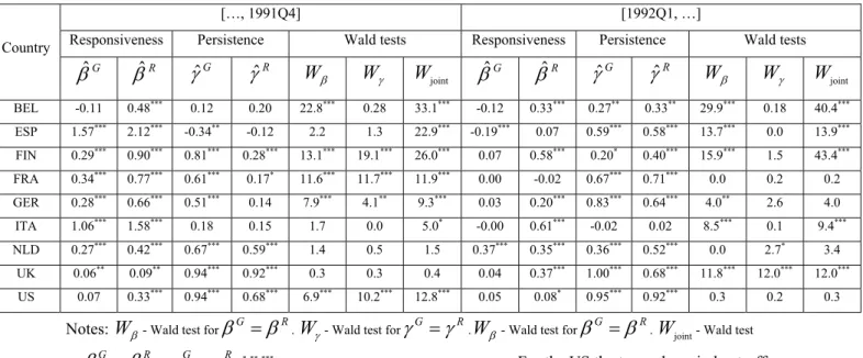
Table 2 – Sub-period estimates for responsiveness and persistence

[…, 1991Q4] [1992Q1, …]

Responsiveness Persistence Wald tests Responsiveness Persistence Wald tests Country G βˆ _βˆR _γ_ˆG _γ_ˆR β W W_γ W_joint _βˆG _βˆR _γ_ˆG _γ_ˆR β W W_γ W_joint BEL -0.11 0.48*** _{0.12 0.20 22.8}*** _{0.28 33.1}*** _{-0.12 0.33}*** _0.27** _0.33** _29.9*** _{0.18 40.4}*** ESP 1.57*** _2.12*** _-0.34** _-0.12 _{2.2 1.3}_22.9*** _-0.19*** _{0.07 0.59}*** _0.58*** _13.7*** _{0.0 13.9}*** FIN 0.29*** _0.90*** _0.81*** _0.28*** _13.1*** _19.1*** _26.0*** _{0.07 0.58}*** _0.20* _0.40*** _15.9*** _{1.5 43.4}*** FRA 0.34*** _0.77*** _0.61*** _0.17* _11.6*** _11.7*** _11.9*** _{0.00 -0.02 0.67}*** _0.71*** _{0.0 0.2 0.2} GER 0.28*** _0.66*** _0.51*** _{0.14 7.9}*** _4.1** _9.3*** _{0.03 0.20}*** _0.83*** _0.64*** _4.0** _{2.6 4.0} ITA 1.06*** _1.58*** _{0.18 0.15 1.7 0.0 5.0}* _{-0.00 0.61}*** _{-0.02 0.02 8.5}*** _{0.1 9.4}*** NLD 0.27*** _0.42*** _0.67*** _0.59*** _{1.4 0.5 1.5}_0.37*** _0.35*** _0.36*** _0.52*** _{0.0 2.7}* _3.4 UK 0.06** _0.09** _0.94*** _0.92*** _{0.3 0.3 0.4 0.04}_0.37*** _1.00*** _0.68*** _11.8*** _12.0*** _12.0*** US 0.07 0.33*** _0.94*** _0.68*** _6.9*** _10.2*** _12.8*** _{0.05 0.08}* _0.95*** _0.92*** _{0.3 0.2 0.3}

Notes: W_β- Wald test forβG =βR. W_{γ - Wald test for}γG =γR.W_β- Wald test forβG =βR. W_joint- Wald test

forβG =βR∧γG =γR. *_,**_,***_{, respectively significant at 10%, 5% and 1%.}_{For the US the two sub-period cut-off}

date is 1987Q3.

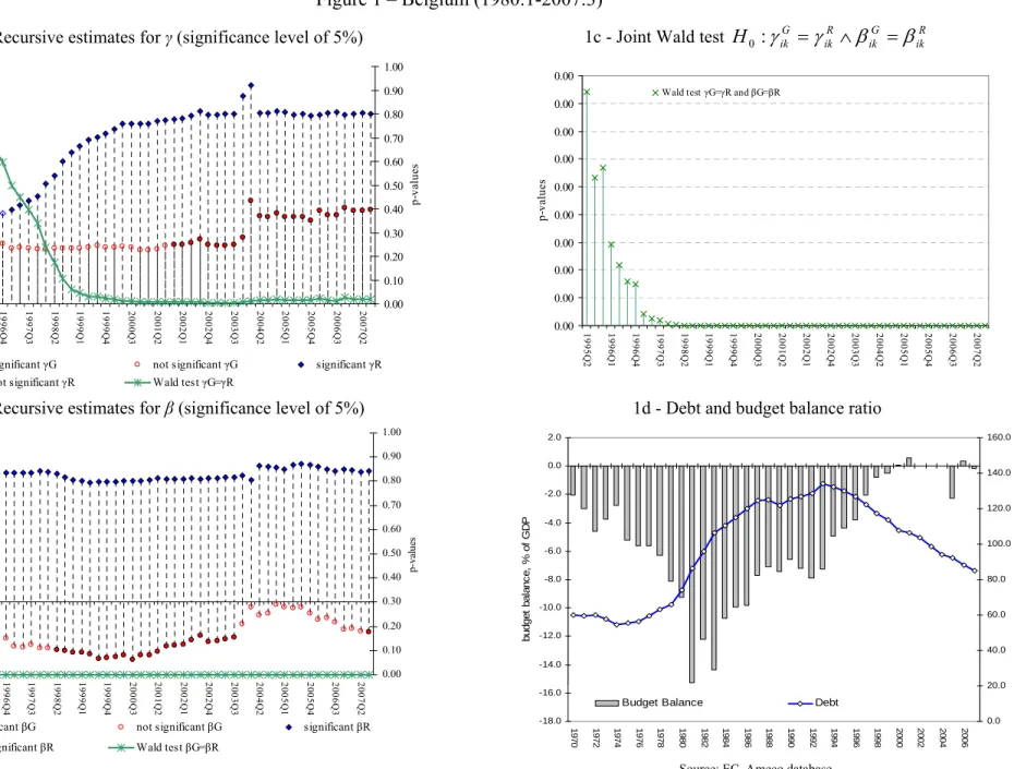
Belgium

The case of Belgium is a particularly interesting one. As it is possible to see from Figure 1d Belgium has been characterized by fiscal deterioration at the beginning of the 1980s, and by fiscal consolidation afterward. Our results seem to confirm this evidence. In Figures 1a and 1b we report the recursive estimates over time of our measures of

(16)

persistence and responsiveness for government spending and revenue. Looking at the figures, we can observe, that the estimates of both persistence and responsiveness of government revenue are higher than the ones of government spending. In particular, Wald tests indicate that the discrepancy in the behaviour of government spending and revenue is highly significant for most of the sample windows (see also Table 1). This suggests that in our period of observation (1980:1-2007:2) fiscal consolidation has occurred in Belgium, and it has been driven by the higher responsiveness and persistence of government revenue, compared to spending. Moreover, splitting the sample period in two sub-periods, before and after the Maastricht Treaty, we can see that fiscal consolidation in both periods has been characterised by higher responsiveness in government revenue (see Table 2).

France

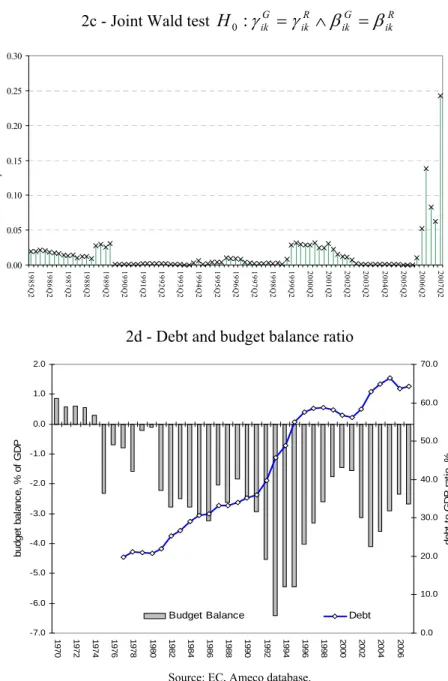
The fiscal balance in France was relatively stable, although in deficit (see Figure 2d), in the first part of the last three decades, at least if compared to other Economic and Monetary Union members (such as Belgium and Italy).

However, our results suggest that a significant fiscal deterioration has occurred during the period 2000-2002 (see Figures 2a, 2b and 2c). Until 1998:4 spending responsiveness is statistically significantly lower than revenue responsiveness and spending persistence is statistically significant bigger than the revenue one, which would imply an overall balanced behaviour. Instead, during the period 2000-2002, government spending persistence is significantly higher that revenue one whilst the null of equality between government spending and government revenue responsiveness is accepted. Indeed, empirical evidence seems to suggest that the periods of fiscal deterioration for France during 2000-2002 are mainly driven by the higher persistence of spending.

(17)

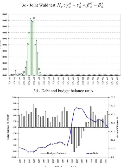
Finland

Public finances have been always quite sound during the last three decades (an exception is represented by the fiscal deterioration during the crisis of the first half of the 1990s). Moreover, looking at Figure 3d, we can see that no major changes in the budget balance seem to have occurred. Our analysis provides similar conclusions, but also shows how this fiscal position has been achieved trough a different behaviour of spending and revenue in terms of responsiveness and persistence (see Figures 3a and 3b). In particular, while government spending persistence has been higher than government revenue persistence, revenue has been more responsive than spending. This is also confirmed by the analysis for the two sub-periods (see Table 1 and 2).

Germany

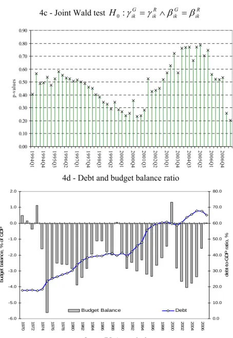
The pattern of the budget balance depicted in Figure 4d, seems to suggest that neither strong fiscal improvements nor deteriorations have occurred in Germany in the last three decades. This hypothesis has been confirmed by our analysis. In fact, as it is possible to see by the joint and the single tests (see Figures 4a, 4b and 4c), the difference, both in terms of responsiveness and persistence, between government spending and revenue is never statistically significant. Moreover, it does not seem that a strikingly different behaviour before and after 1992 has emerged (see Table 2). Nevertheless, it is interesting to observe that magnitude of government revenue responsiveness declined after 2000-2001, while it remained rather stable for government spending, somewhat anticipating a situation of lower revenues and the Excessive Deficit Procedure that Germany faced in 2002.7

7_{Afonso and Claeys (2007) mention that a large revenue reduction, unmatched by expenditure cuts in}

(18)

Italy

Budget deficits have been considerably high and increasing during the 1970s and the 1980s, and only started decreasing after the beginning of the 1990s (see Figure 5d). Our analysis, which starts in 1980:1, uncovers empirical evidence for fiscal consolidation in the period after the Maastricht Treaty (see Table 2). Moreover, from the analysis of the coefficients and the associated Wald tests, we can argue that fiscal improvements in the second half of the 1990s have been achieved rather through higher revenue responsiveness (see Figure 5b). Indeed, the null hypothesis of identical government revenue and spending responsiveness is mostly rejected after 1997.

Netherlands

Fiscal balances have improved in the Netherlands in the 1990s, after some deterioration in the 1980s. This is (partly) captured by our analysis. In particular, looking at the pattern of the estimates of responsiveness and persistence, we can see that around 1996 government revenue has become more persistent than government spending, after several years where the situation was the opposite (see Figure 6a). In contrast, regarding responsiveness, government revenue and spending do not seem to have differed in statistically significant terms (see Figure 6b), apart from the period 2000:2-2001:3, when spending responsiveness decreased and the budget position improved (see Figure 6d).

Spain

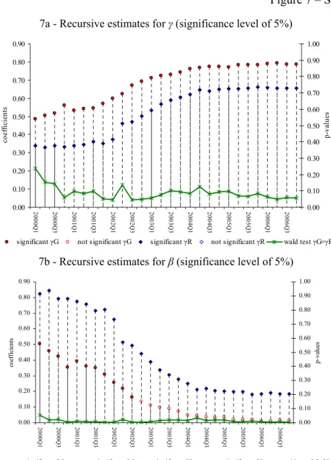
Analyzing the pattern for fiscal budget balances in Spain, we can see that there has been a process of fiscal consolidation from 1995 onwards. In fact the budget deficit passed from above 6% of GDP in 1995 to a surplus of 2.3% of GDP in 2007. The joint test of our measure of persistence confirms this outcome (see Figure 7c). However, and for the period

(19)

of analysis, we can reject that the measures of persistence and responsiveness are the same (see Figure 7c). In particular, while government spending has been more persistent than government revenue, revenue was more responsive than spending. This, together with the fact that the levels of deficit and debt have been reduced over time, seems to point out that the higher responsiveness of revenue more than balanced the higher persistence of spending.

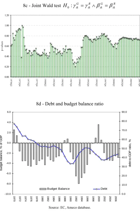
United Kingdom

Fiscal balances in the UK have been quite stable with the debt-to-GDP ratio decreasing throughout the 1970s and 1980s (see Figure 8d). In particular, except for 2000 and 2001 (due to relatively high GDP growth), it is possible to argue that there has not been any significant changes towards fiscal improvement or deterioration. This was mainly due to the fact that higher government spending and revenue showed a very similar behaviour in terms of persistence and responsiveness (see Figures 8a and 8b).

USA

Similarly to the UK, the fiscal balances in the U.S. have been quite stable, although in deficit, with an improvement of the fiscal position between 1992 and 2000 (see Figure 9d). Overall, it is possible to argue that there has not been any significant long-term change towards fiscal consolidation or deterioration. Unlike the case of UK, however, this was due to the fact that higher revenue responsiveness has been balanced by higher spending persistence (see Figures 9a and 9b).

5. Conclusion

In this work, we propose a new approach to assess long-term fiscal developments. By analyzing the time-varying behaviour of the two components of government spending

(20)

and revenues – that is, responsiveness and persistence –, we are able to infer about the sources of fiscal deterioration and/or fiscal improvement. Drawing on quarterly data we use a Three-Stage Least Square method and recursively estimate those components within a system of government revenue and spending equations.

The results suggest that fiscal deterioration has not been an issue for the majority of the countries analyzed. In fact, fiscal position has not significantly changed for Finland, France, Germany, Spain, the United Kingdom and the US, whilst it has even improved for Belgium, Italy, and Netherlands.

We show that, for Italy, Belgium and (partially) for the Netherlands, fiscal improvement has been mainly driven by a higher responsiveness of government revenue relative to government spending. On the other hand, in the case of France, periods of fiscal deterioration can be attributed to the higher persistence of spending. This result is in line with the argument that although revenue is more responsive than spending, spending is more persistent than revenue (see Afonso, et al. 2008).

Additionally, we have not detected conditions for potential fiscal deterioration or fiscal improvement in the other European Union countries (Finland, Germany, Spain, and the UK) plus the U.S. For these countries, the empirical evidence suggests that non-significant change in the fiscal position is due to a similar behaviour in terms of persistence and responsiveness of government spending and government revenue or because higher revenue responsiveness has been balanced by higher spending persistence.

References

Afonso, A. (2005). “Fiscal Sustainability: the Unpleasant European Case”, FinanzArchiv, 61 (1), 19-44.

Afonso, A. (2008). “Ricardian Fiscal Regimes in the European Union”, Empirica, 35 (3), 313–334.

(21)

Afonso, A. and Claeys, P. (2007). “The dynamic behaviour of budget components and output”, Economic Modelling, 25, 93-117.

Afonso, A. and Rault, C. (2007). “What do we really know about fiscal sustainability in the EU? A panel data diagnostic”, ECB Working Paper n. 820.

Afonso, A. and Rault, C. (2008). “3-step Analysis of Public Finances Sustainability: the Case of the European Union”, ECB Working Paper n. 908.

Afonso, A. and Sousa, R. (2009). “The macroeconomic effects of fiscal policy”, ECB Working Paper n. 991.

Afonso, A.; Agnello, A.; and Furceri, D. (2008). “Fiscal Policy Responsiveness, Persistence and Discretion”, ECB Working Paper 954.

Ahmed, S., and Rogers, J. (1995). “Government Budget Deficits and Trade Deficits. Are Present Value Constraints Satisfied in Long-term Data?” Journal of Monetary

Economics 36, 351–374.

Biau, O. and Girard, E. (2005). “Politique budgétaire et dynamique économique en France: l'approche VAR structurel”, Économie et Prévision, 169–171, 1–24.

Baglioni, A., and Cherubini, U. (1993). “Intertemporal Budget Constraint and Public Debt Sustainability: The Case of Italy,” Applied Economics 25, 275–283.

Bohn, H. (1991). “The Sustainability of Budget Deficits with Lump-Sum and with Income-Based Taxation”, Journal of Money, Credit, and Banking 23, 581–604.

Bohn, H. (2007). “Are stationarity and cointegration restrictions really necessary for the intertemporal budget constraint?” Journal of Monetary Economics, 54 (7), 1837-1847. De Castro Fernández, F. and Hernández de Cos, P. (2006). “The economic effects of

exogenous fiscal shocks in Spain: a SVAR approach”, ECB Working Paper 647.

Fatás, A. and Mihov, I. (2003). “The Case for Restricting Fiscal Policy Discretion”,

Quarterly Journal of Economics, 118, 1419-1447.

Fatás, A. and Mihov, I. (2006). “The Macroeconomics Effects of Fiscal Rules in the US States”, Journal of Public Economics, 90, 101-117.

Giordano, R.; Momigliano, S.; Neri, S.; Perotti, R. (2007). “The effects of fiscal policy in Italy: Evidence from a VAR model”, European Journal of Political Economy, 23, 707-733.

Heppke-Falk, K..; Tenhofen, J.; Wolff, G. (2006). “The macroeconomic effects of exogenous fiscal policy shocks in Germany: a disaggregated SVAR analysis”, Deutsche Bundesbank, Discussion Paper 41.

(22)

Hakkio, G., and Rush, M. (1991). “Is the Budget Deficit Too Large?” Economic Inquiry 29, 429–445.

Hamilton, J., and Flavin, M. (1986). “On the Limitations of Government Borrowing: A Framework for Empirical Testing”, American Economic Review 76, 808–816.

Hatemi-J, A. (2002). “Fiscal Policy in Sweden: Effects of EMU Criteria Convergence”,

Economic Modelling 19, 121–136.

Haug, A. (1995). “Has Federal Budget Deficit Policy Changed in Recent Years?”

Economic Inquiry 33, 104–118.

MacDonald, R. (1992). “Some Tests of the Government’s Intertemporal Budget Constraint Using U.S. Data”, Applied Economics 24, 1287-1292.

Olekalns, N. (2000). “Sustainability and Stability? Australian Fiscal Policy in the 20th Century,” Australian Economic Papers 39, 138–151.

Onorante, L., Pedregal, D., Pérez, J, and Signorini, S. (2008). “The usefulness of infra-annual government cash budgetary data for fiscal forecasting in the euro area”, ECB Working Paper n. 901.

Pérez, J. (2007). “Leading indicators for euro area government deficits”, International

Journal of Forecasting, 23, 259-275.

Quintos, C. (1995). “Sustainability of the Deficit Process with Structural Shifts”, Journal

of Business & Economic Statistics 13, 409–417.

Smith, G., and Zin, S. (1991). “Persistent Deficits and the Market Value of Government Debt,” Journal of Applied Econometrics 6, 31–44.

Trehan, B., and Walsh, C. (1988). “Common Trends, the Government’s Budget Constraint, and Revenue Smoothing”, Journal of Economic Dynamics and Control 12, 425–444.

Trehan, B., and Walsh, C. (1991). “Testing Intertemporal Budget Constraints: Theory and Applications to U.S. Federal Budget and Current Account Deficits”, Journal of Money,

Credit, and Banking 23, 206–223.

Wirjanto, T., and Amano, R. (1996). “Nonstationary regression models with a lagged dependent variable”, Communications in statistics. Theory and methods, 25 (7), 1489-1503.

Zellner, A. and Theil, H. (1962). “Three Stage Least Squares: Simultaneous Estimation of Simultaneous Equations”, Econometrica, 30 (1), 54-78.

(23)

Appendix. Data description and sources A.1 Belgium Data

GDP

The source is the IMF, International Financial Statistics (series " IFS.Q.124.9.9B.B$$.Z.W.$$$"). We seasonally adjust quarterly data using Census X12 ARIMA, and the series comprise the period 1980:1-2007:3.

Price Deflator

All variables were deflated by the GDP deflator (2000=100). The source is the IMF, International Financial Statistics (series IFS.Q.124.9.9B.BIP.Z.F.$$$”). We seasonally adjust quarterly data using Census X12 ARIMA, and the series comprise the period 1980:1-2007:3.

Government Spending

The source is the Belgium Ministry of Finance. Government Spending is defined as State Government expenditure on a cash basis (series “BISM.M.FJHC.BE.91”). We seasonally adjust quarterly data using Census X12 ARIMA, and the series comprise the period 1967:1-2008:1.

Government Revenue

The source is the Belgium Ministry of Finance. Government Revenue is defined as State Government revenue on a cash basis (series “BISM.M.FJBC.BE.91”). We seasonally adjust quarterly data using Census X12 ARIMA, and the series comprise the period 1967:1-2008:1.

A.2 Finland Data GDP

The source is the IMF, International Financial Statistics (series " IFS.Q.172.9.9B.B$$.Z.W.$$$"). We seasonally adjust quarterly data using Census X12 ARIMA, and the series comprise the period 1970:1-2007:4

Price Deflator

All variables were deflated by the GDP deflator (2000=100). The source is the IMF, International Financial Statistics (series “IFS.Q.172.9.9B.BIP.Z.F.$$”). We seasonally adjust quarterly data using Census X12 ARIMA, and the series comprise the period 1970:1-2007:4.

The source is the IMF via Finnish Ministry of Finance. Government Spending is defined as State Government expenditure on a cash basis (series “IFS.M.17282...ZF...”). We seasonally adjust quarterly data using Census X12 ARIMA, and the series comprise the period 1970:1-2007:4.

The source is the IMF via Finnish Ministry of Finance. Government Revenue is defined as State Government revenue on a cash basis (series “IFS.M.17281...ZF...”). We seasonally

(24)

adjust quarterly data using Census X12 ARIMA, and the series comprise the period 1970:1-2007:4.

A.3 France Data GDP

Data for GDP are quarterly, seasonally adjusted, and comprise the period 1970:1-2007:2. The source is the IMF, International Financial Statistics (series " IFS.Q.132.9.9B.B$C.Z.F.$$$").

Price Deflator

All variables were deflated by the GDP deflator (2000=100). Data are quarterly, seasonally adjusted, and comprise the period 1970:1-2007:2. The source is the IMF, International Financial Statistics (series “IFS.Q.132.9.9B.BIR.Z.F.$$$”).

The source is the IMF via French Ministry of Finance. Government Spending is defined as State Government expenditure on a cash basis (series “IFS.M.13282z..ZF...”). We seasonally adjust quarterly data using Census X12 ARIMA, and the series comprise the period 1970:1-2007:2.

The source is the IMF via French Ministry of Finance. Government Revenue is defined as State Government revenue on a cash basis (series “IFS.M.13281...ZF...”). We seasonally adjust quarterly data using Census X12 ARIMA, and the series comprise the period 1970:1-2007:2.

A.4 Germany Data GDP

Data for GDP are quarterly, seasonally adjusted, and comprise the period 1960:1-2007:4. The source is the IMF, International Financial Statistics (series "IFS.Q.134.9.9B.B$C.Z.F.$$$").

Price Deflator

All variables were deflated by the GDP deflator (2000=100). Data are quarterly, seasonally adjusted, and comprise the period 1960:1-2007:2. The source is the IMF, International Financial Statistics (series "IFS.Q.134.9.9B.BIR.Z.F.$$$”).

The source is the Bundesbank and the Monthly Reports released by the German Ministry of Finance. Government Spending is defined as General Government total expenditure on a cash basis. We seasonally adjust quarterly data using Census X12 ARIMA, and the series comprise the period 1979:1-2007:3.

The source is the Bundesbank and the Monthly Reports released by the German Ministry of Finance. Government Revenue is defined as General Government total revenue on a cash basis. We seasonally adjust quarterly data using Census X12 ARIMA, and the series comprise the period 1979:1-2007:3.

(25)

A.5 Italy Data GDP

Data for GDP are quarterly, seasonally adjusted, and comprise the period 1960:1-2007:3. The source is the IMF, International Financial Statistics (series "IFS.Q.136.9.9B.B$C.Z.F.$$$").

Price Deflator

The source is the Bank of Italy and the Italian Ministry of Finance. Government Spending is defined as Central Government primary expenditure on a cash basis. We seasonally adjust quarterly data using Census X12 ARIMA, and the series comprise the period 1960:1-2007:4.

The source is the Bank of Italy and the Italian Ministry of Finance. Government Revenue is defined as Central Government total revenue on a cash basis. We seasonally adjust quarterly data using Census X12 ARIMA, and the series comprise the period 1960:1-2007:4.

A.6 Spain Data GDP

Data for GDP are quarterly, seasonally adjusted, and comprise the period 1970:1-2007:2. The source is the IMF, International Financial Statistics (series " IFS.Q.184.9.9B.B$C.Z.F.$$$").

Price Deflator

The source is the IMF via Spanish Ministry of Finance. Government Spending is defined as State Government expenditure on a cash basis (series “IFS.M.18482...Zf...”). We seasonally adjust quarterly data using Census X12 ARIMA, and the series comprise the period 1985:1-2006:4.

The source is the IMF via Spanish Ministry of Finance. Government Revenue is defined as State Government revenue on a cash basis (series “IFS.M.18481...Zf...”). We seasonally adjust quarterly data using Census X12 ARIMA, and the series comprise the period 1986:1-2006:4.

(26)

A.7 Netherlands Data GDP

The source is the IMF, International Financial Statistics (series " IFS.Q.138.9.9B.B$C.Z.W.$$$"). We seasonally adjust quarterly data using Census X12 ARIMA, and the series comprise the period 1970:1-2007:4.

Price Deflator

All variables were deflated by the GDP deflator (2000=100). The source is the IMF, International Financial Statistics (series “IFS.Q.138.9.9B.BIR.Z.F.$$$”). We seasonally adjust quarterly data using Census X12 ARIMA, and the series comprise the period 1970:1-2007:2.

The source is the IMF via Dutch Ministry of Finance. Government Spending is defined as State Government expenditure on a cash basis (series “IFS.M.138.C.C2.$$$.C.G.$$$”). We seasonally adjust quarterly data using Census X12 ARIMA, and the series comprise the period 1970:1-2007:1.

The source is the IMF via Dutch Ministry of Finance. Government Revenue is defined as State Government revenue on a cash basis (series “IFS.M.138.C.C1.$$$.C.G.$$$”). We seasonally adjust quarterly data using Census X12 ARIMA, and the series comprise the period 1970:1-2007:1.

A.8 U.K. Data GDP

Data for GDP are quarterly, seasonally adjusted, and comprise the period 1955:1-2007:4. The source is the Office for National Statistics, Release UKEA, Table A1 (series "YBHA").

Price Deflator

All variables were deflated by the GDP deflator. Data are quarterly, seasonally adjusted, and comprise the period 1955:1-2007:4. The source is the Office for National Statistics, Release MDS, Table 1.1 (series “YBGB”).

The source is the Office for National Statistics (ONS), Release Public Sector Accounts. Government Spending is defined as total current expenditures of the Public Sector ESA 95 (series “ANLT”) less net investment (series “ANNW”). We seasonally adjust quarterly data using Census X12 ARIMA, and the series comprise the period 1947:1-2007:4.

The source is the Office for National Statistics (ONS), Release Public Sector Accounts. Government Revenue is defined as total current receipts of the Public Sector ESA 95 (series “ANBT”). We seasonally adjust quarterly data using Census X12 ARIMA, and the series comprise the period 1947:1-2007:4.

(27)

A.9 U.S. Data GDP

The source is Bureau of Economic Analysis, NIPA Table 1.1.5, line 1. Data for GDP are quarterly, seasonally adjusted, and comprise the period 1947:1-2007:4.

Price Deflator

All variables were deflated by the GDP deflator. Data are quarterly, seasonally adjusted, and comprise the period 1967:1-2007:4. The source is the Bureau of Economic Analysis, NIPA Tables 1.1.5 and 1.1.6, line 1.

The source is Bureau of Economic Analysis, NIPA Table 3.2. Government Spending is defined as total Federal Government Current Expenditure (line 39). Data are quarterly, seasonally adjusted, and comprise the period 1960:1-2007:4.

The source is Bureau of Economic Analysis, NIPA Table 3.2. Government Revenue is defined as government receipts at annual rates (line 36). Data are quarterly, seasonally adjusted, and comprise the period 1947:1-2007:4.

(28)

Figure 1 – Belgium (1980:1-2007:3)

1a - Recursive estimates for γ (significance level of 5%) 1c - Joint Wald test H₀ :γ_ikG =γ_ikR ∧β_ikG =β_ikR

0.00 0.10 0.20 0.30 0.40 0.50 0.60 199 5Q 2 199 6Q 1 199 6Q 4 199 7Q 3 199 8Q 2 199 9Q 1 199 9Q 4 200 0Q 3 200 1Q 2 200 2Q 1 200 2Q 4 200 3Q 3 200 4Q 2 200 5Q 1 200 5Q 4 200 6Q 3 200 7Q 2 co ef fi ci en ts 0.00 0.10 0.20 0.30 0.40 0.50 0.60 0.70 0.80 0.90 1.00 p-va lu es

significant γG not significant γG significant γR not significant γR Wald test γG=γR

0.00 0.00 0.00 0.00 0.00 0.00 0.00 0.00 0.00 0.00 19 95Q 2 19 96Q 1 19 96Q 4 19 97Q 3 19 98Q 2 19 99Q 1 19 99Q 4 20 00Q 3 20 01Q 2 20 02Q 1 20 02Q 4 20 03Q 3 20 04Q 2 20 05Q 1 20 05Q 4 20 06Q 3 20 07Q 2 p-va lu es

Wald test γG=γR and βG=βR

1b - Recursive estimates for β (significance level of 5%) 1d - Debt and budget balance ratio

-0.30 -0.20 -0.10 0.00 0.10 0.20 0.30 0.40 0.50 0.60 0.70 199 5Q 2 199 6Q 1 199 6Q 4 199 7Q 3 199 8Q 2 199 9Q 1 199 9Q 4 200 0Q 3 200 1Q 2 200 2Q 1 200 2Q 4 200 3Q 3 200 4Q 2 200 5Q 1 200 5Q 4 200 6Q 3 200 7Q 2 co ef fi cie nts 0.00 0.10 0.20 0.30 0.40 0.50 0.60 0.70 0.80 0.90 1.00 p-v al ue s

significant βG not significant βG significant βR not significant βR Wald test βG=βR

-18.0 -16.0 -14.0 -12.0 -10.0 -8.0 -6.0 -4.0 -2.0 0.0 2.0 1 970 1972 1974 1976 9781 1980 1982 1984 1986 9881 1990 1992 1994 1996 1998 2000 2002 2004 2006 bu dg et ba la nc e, % o f GD P 0.0 20.0 40.0 60.0 80.0 100.0 120.0 140.0 160.0 de bt -t o-G D P r a ti o , %

Budget Balance Debt

(29)

Figure 2 – France (1970:2-2007:2)

0.00 0.10 0.20 0.30 0.40 0.50 0.60 0.70 0.80 1985Q 2 1986Q 1 1986Q 4 1987Q 3 1988Q 2 1989Q 1 1989Q 4 1990Q 3 1991Q 2 1992Q 1 1992Q 4 1993Q 3 1994Q 2 1995Q 1 1995Q 4 1996Q 3 1997Q 2 1998Q 1 1998Q 4 1999Q 3 2000Q 2 2001Q 1 2001Q 4 2002Q 3 2003Q 2 2004Q 1 2004Q 4 2005Q 3 2006Q 2 2007Q 1 co ef fi cien ts 0.00 0.10 0.20 0.30 0.40 0.50 0.60 0.70 0.80 0.90 1.00 p-va lu es

significant γG not significant γG significant γR not significant γR wald test γG=γR

0.00 0.05 0.10 0.15 0.20 0.25 0.30 19 85 Q 2 19 86 Q 2 19 87 Q 2 19 88 Q 2 19 89 Q 2 19 90 Q 2 19 91 Q 2 19 92 Q 2 19 93 Q 2 19 94 Q 2 19 95 Q 2 19 96 Q 2 19 97 Q 2 19 98 Q 2 19 99 Q 2 20 00 Q 2 20 01 Q 2 20 02 Q 2 20 03 Q 2 20 04 Q 2 20 05 Q 2 20 06 Q 2 20 07 Q 2 p-va lu es

2b - Recursive estimates for β (significant level of 5%) 2d - Debt and budget balance ratio

0.00 0.10 0.20 0.30 0.40 0.50 0.60 0.70 0.80 0.90 1985Q 2 1986Q 1 1986Q 4 1987Q 3 1988Q 2 1989Q 1 1989Q 4 1990Q 3 1991Q 2 1992Q 1 1992Q 4 1993Q 3 1994Q 2 1995Q 1 1995Q 4 1996Q 3 1997Q 2 1998Q 1 1998Q 4 1999Q 3 2000Q 2 2001Q 1 2001Q 4 2002Q 3 2003Q 2 2004Q 1 2004Q 4 2005Q 3 2006Q 2 2007Q 1 co ef fi ci en ts 0.00 0.10 0.20 0.30 0.40 0.50 0.60 0.70 0.80 0.90 1.00 p-va lue s

significant βG not significant βG significant βR not significant βR wald test βG=βR -7.0 -6.0 -5.0 -4.0 -3.0 -2.0 -1.0 0.0 1.0 2.0 19 70 19 72 19 74 19 76 19 78 19 80 19 82 19 84 19 86 19 88 19 90 19 92 19 94 19 96 19 98 20 00 20 02 20 04 20 06 budget bal anc e, % of G D P 0.0 10.0 20.0 30.0 40.0 50.0 60.0 70.0 debt -t o-G D P rat io, %

Budget Balance Debt

(30)

Figure 3 – Finland (1970:1-2007:4)

0.00 0.10 0.20 0.30 0.40 0.50 0.60 0.70 0.80 0.90 1.00 19 85 Q 2 19 86 Q 2 19 87 Q 2 19 88 Q 2 19 89 Q 2 19 90 Q 2 19 91 Q 2 19 92 Q 2 19 93 Q 2 19 94 Q 2 19 95 Q 2 19 96 Q 2 19 97 Q 2 19 98 Q 2 19 99 Q 2 20 00 Q 2 20 01 Q 2 20 02 Q 2 20 03 Q 2 20 04 Q 2 20 05 Q 2 20 06 Q 2 20 07 Q 2 co ef fi ci en ts 0.00 0.10 0.20 0.30 0.40 0.50 0.60 0.70 0.80 0.90 1.00 p-va lu es

0.00 0.00 0.00 0.00 0.00 0.00 0.00 0.00 0.00 0.00 0.00 19 85Q 2 19 86Q 2 19 87Q 2 19 88Q 2 19 89Q 2 19 90Q 2 19 91Q 2 19 92Q 2 19 93Q 2 19 94Q 2 19 95Q 2 19 96Q 2 19 97Q 2 19 98Q 2 19 99Q 2 20 00Q 2 20 01Q 2 20 02Q 2 20 03Q 2 20 04Q 2 20 05Q 2 20 06Q 2 20 07Q 2 p-va lu es

3b - Recursive estimates for β (significant level of 5%) 3d - Debt and budget balance ratio

0.00 0.20 0.40 0.60 0.80 1.00 1.20 1985Q 2 1986Q 2 1987Q 2 1988Q 2 1989Q 2 1990Q 2 1991Q 2 1992Q 2 1993Q 2 1994Q 2 1995Q 2 1996Q 2 1997Q 2 1998Q 2 1999Q 2 2000Q 2 2001Q 2 2002Q 2 2003Q 2 2004Q 2 2005Q 2 2006Q 2 2007Q 2 co ef fi ci en ts 0.00 0.10 0.20 0.30 0.40 0.50 0.60 0.70 0.80 0.90 1.00 p-va lu es

significant βG not significant βG significant βR not significant βR wald test βG=βR

-10.0 -8.0 -6.0 -4.0 -2.0 0.0 2.0 4.0 6.0 8.0 10.0 19 70 19 72 19 74 19 76 19 78 19 80 19 82 19 84 19 86 19 88 19 90 19 92 19 94 19 96 19 98 20 00 20 02 20 04 20 06 bu dg et b a lanc e, % of G D P 0.0 10.0 20.0 30.0 40.0 50.0 60.0 70.0 de bt -t o -G D P r a ti o, %

Budget Balance Debt

(31)

Figure 4 – Germany (1979:1-2007:2)

0.00 0.10 0.20 0.30 0.40 0.50 0.60 0.70 0.80 19 94 Q 1 19 94 Q 4 19 95 Q 3 19 96 Q 2 19 97 Q 1 19 97 Q 4 19 98 Q 3 19 99 Q 2 20 00 Q 1 20 00 Q 4 20 01 Q 3 20 02 Q 2 20 03 Q 1 20 03 Q 4 20 04 Q 3 20 05 Q 2 20 06 Q 1 20 06 Q 4 co ef fi cien ts 0.00 0.10 0.20 0.30 0.40 0.50 0.60 0.70 0.80 0.90 1.00 p-va lu es

0.00 0.10 0.20 0.30 0.40 0.50 0.60 0.70 0.80 0.90 1994Q 1 1994Q 4 1995Q 3 1996Q 2 1997Q 1 1997Q 4 1998Q 3 1999Q 2 2000Q 1 2000Q 4 2001Q 3 2002Q 2 2003Q 1 2003Q 4 2004Q 3 2005Q 2 2006Q 1 2006Q 4 p-va lu es

0.00 0.05 0.10 0.15 0.20 0.25 0.30 0.35 19 94Q 1 19 94Q 4 19 95Q 3 19 96Q 2 19 97Q 1 19 97Q 4 19 98Q 3 19 99Q 2 20 00Q 1 20 00Q 4 20 01Q 3 20 02Q 2 20 03Q 1 20 03Q 4 20 04Q 3 20 05Q 2 20 06Q 1 20 06Q 4 co ef fi ci en ts 0.00 0.10 0.20 0.30 0.40 0.50 0.60 0.70 0.80 0.90 1.00 p-va lu es

-6.0 -5.0 -4.0 -3.0 -2.0 -1.0 0.0 1.0 2.0 19 70 19 72 19 74 19 76 19 78 19 80 19 82 19 84 19 86 19 88 19 90 19 92 19 94 19 96 19 98 20 00 20 02 20 04 20 06 bu dget b a la n c e, % of G D P 0.0 10.0 20.0 30.0 40.0 50.0 60.0 70.0 80.0 de bt -t o-G D P r a ti o , %

Budget Balance Debt

(32)

Figure 5 – Italy (1980:1-2007:3)

-0.10 -0.05 0.00 0.05 0.10 0.15 0.20 0.25 0.30 0.35 0.40 0.45 1995Q 2 1996Q 1 1996Q 4 1997Q 3 1998Q 2 1999Q 1 1999Q 4 2000Q 3 2001Q 2 2002Q 1 2002Q 4 2003Q 3 2004Q 2 2005Q 1 2005Q 4 2006Q 3 2007Q 2 co ef fi ci en ts 0.00 0.10 0.20 0.30 0.40 0.50 0.60 0.70 0.80 0.90 1.00 p-va lu es

0.00 0.00 0.00 0.00 0.00 0.00 0.00 0.00 0.00 1995Q 2 1995Q 4 1996Q 2 1996Q 4 1997Q 2 1997Q 4 1998Q 2 1998Q 4 1999Q 2 1999Q 4 2000Q 2 2000Q 4 2001Q 2 2001Q 4 2002Q 2 2002Q 4 2003Q 2 2003Q 4 2004Q 2 2004Q 4 2005Q 2 2005Q 4 2006Q 2 2006Q 4 2007Q 2 p-va lue s

0.00 0.20 0.40 0.60 0.80 1.00 1.20 1.40 1.60 1995Q 2 1996Q 1 1996Q 4 1997Q 3 1998Q 2 1999Q 1 1999Q 4 2000Q 3 2001Q 2 2002Q 1 2002Q 4 2003Q 3 2004Q 2 2005Q 1 2005Q 4 2006Q 3 2007Q 2 co ef fi ci en ts 0.00 0.10 0.20 0.30 0.40 0.50 0.60 0.70 0.80 0.90 1.00 p-va lu es

-14.0 -12.0 -10.0 -8.0 -6.0 -4.0 -2.0 0.0 1 970 1972 1974 1976 9781 1980 1982 1984 1986 9881 1990 1992 1994 1996 1998 2000 2002 2004 2006 bu dg et ba la n c e , % o f G D P 0.0 20.0 40.0 60.0 80.0 100.0 120.0 140.0 de bt -t o-G D P r a ti o , %

Budget Balance Debt

(33)

Figure 6 – Netherlands (1977:1-2007:1)

0.00 0.10 0.20 0.30 0.40 0.50 0.60 0.70 0.80 1992Q 2 1993Q 1 1993Q 4 1994Q 3 1995Q 2 1996Q 1 1996Q 4 1997Q 3 1998Q 2 1999Q 1 1999Q 4 2000Q 3 2001Q 2 2002Q 1 2002Q 4 2003Q 3 2004Q 2 2005Q 1 2005Q 4 2006Q 3 co ef fi cie nt s 0.00 0.10 0.20 0.30 0.40 0.50 0.60 0.70 0.80 0.90 1.00 p-va lu es

0.00 0.10 0.20 0.30 0.40 0.50 0.60 19 92 Q 2 19 92 Q 4 19 93 Q 2 19 93 Q 4 19 94 Q 2 19 94 Q 4 19 95 Q 2 19 95 Q 4 19 96 Q 2 19 96 Q 4 19 97 Q 2 19 97 Q 4 19 98 Q 2 19 98 Q 4 19 99 Q 2 19 99 Q 4 20 00 Q 2 20 00 Q 4 20 01 Q 2 20 01 Q 4 20 02 Q 2 20 02 Q 4 20 03 Q 2 20 03 Q 4 20 04 Q 2 20 04 Q 4 20 05 Q 2 20 05 Q 4 20 06 Q 2 20 06 Q 4 p-va lu es

0.00 0.05 0.10 0.15 0.20 0.25 0.30 0.35 0.40 0.45 0.50 1992Q 2 1993Q 1 1993Q 4 1994Q 3 1995Q 2 1996Q 1 1996Q 4 1997Q 3 1998Q 2 1999Q 1 1999Q 4 2000Q 3 2001Q 2 2002Q 1 2002Q 4 2003Q 3 2004Q 2 2005Q 1 2005Q 4 2006Q 3 co ef fi ci en ts 0.00 0.10 0.20 0.30 0.40 0.50 0.60 0.70 0.80 0.90 1.00 p-va lu es

significant βG not significant βG significant βR not significant βR wald test βG=βR -7.0 -6.0 -5.0 -4.0 -3.0 -2.0 -1.0 0.0 1.0 2.0 3.0 1970 1972 1974 1976 1978 1980 1982 1984 1986 1988 1990 1992 1994 1996 1998 2000 2002 2004 2006 budget bal anc e, % of G D P 0.0 10.0 20.0 30.0 40.0 50.0 60.0 70.0 80.0 90.0 debt -t o-G D P r a ti o, %

Budget Balance Debt

(34)

Figure 7 – Spain (1985:1-2006:4)

0.00 0.10 0.20 0.30 0.40 0.50 0.60 0.70 0.80 0.90 20 00 Q 1 20 00 Q 3 20 01 Q 1 20 01 Q 3 20 02 Q 1 20 02 Q 3 20 03 Q 1 20 03 Q 3 20 04 Q 1 20 04 Q 3 20 05 Q 1 20 05 Q 3 20 06 Q 1 20 06 Q 3 co ef fi ci en ts 0.00 0.10 0.20 0.30 0.40 0.50 0.60 0.70 0.80 0.90 1.00 p-va lu es

0.00 0.02 0.04 0.06 0.08 0.10 0.12 2000Q 1 2000Q 3 2001Q 1 2001Q 3 2002Q 1 2002Q 3 2003Q 1 2003Q 3 2004Q 1 2004Q 3 2005Q 1 2005Q 3 2006Q 1 2006Q 3 p-va lu es

0.00 0.10 0.20 0.30 0.40 0.50 0.60 0.70 0.80 0.90 200 0Q 1 200 0Q 3 200 1Q 1 200 1Q 3 200 2Q 1 200 2Q 3 200 3Q 1 200 3Q 3 200 4Q 1 200 4Q 3 200 5Q 1 200 5Q 3 200 6Q 1 200 6Q 3 co ef fi cie nt s 0.00 0.10 0.20 0.30 0.40 0.50 0.60 0.70 0.80 0.90 1.00 p-va lu es

-8.0 -7.0 -6.0 -5.0 -4.0 -3.0 -2.0 -1.0 0.0 1.0 2.0 3.0 197 0 197 2 197 4 197 6 197 8 198 0 198 2 198 4 198 6 198 8 199 0 199 2 199 4 199 6 199 8 200 0 200 2 200 4 200 6 budget bal anc e, % of G D P 0.0 10.0 20.0 30.0 40.0 50.0 60.0 70.0 80.0 debt -t o-G D P r a ti o, %

(35)

Figure 8 – United Kingdom (1955:2-2007:4)

0.00 0.20 0.40 0.60 0.80 1.00 1.20 19 70Q2 1972Q4 1975Q2 1977Q4 1980Q2 1982Q4 1985Q2 1987Q4 1990Q2 1992Q4 1995Q2 1997Q4 2000Q2 2002Q4 2005Q2 2007Q4 co ef fi ci en ts 0.00 0.10 0.20 0.30 0.40 0.50 0.60 0.70 0.80 0.90 1.00 p-va lu es

0.00 0.20 0.40 0.60 0.80 1.00 1.20 1970 Q 2 1972 Q 4 1975 Q 2 1977 Q 4 1980 Q 2 1982 Q 4 1985 Q 2 1987 Q 4 1990 Q 2 1992 Q 4 1995 Q 2 1997 Q 4 2000 Q 2 2002 Q 4 2005 Q 2 2007 Q 4 p-va lu es

0.00 0.05 0.10 0.15 0.20 0.25 0.30 0.35 0.40 0.45 19 70 Q2 19 72 Q4 19 75 Q2 19 77 Q4 19 80 Q2 19 82 Q4 19 85 Q2 19 87 Q4 19 90 Q2 19 92 Q4 19 95 Q2 19 97 Q4 20 00 Q2 20 02 Q4 20 05 Q2 20 07 Q4 co ef fi cien ts 0.00 0.10 0.20 0.30 0.40 0.50 0.60 0.70 0.80 0.90 1.00 p-va lu es

-10.0 -8.0 -6.0 -4.0 -2.0 0.0 2.0 4.0 6.0 19 70 19 72 19 74 19 76 19 78 19 80 19 82 19 84 19 86 19 88 19 90 19 92 19 94 19 96 19 98 20 00 20 02 20 04 20 06 budget bal anc e, % of GD P 0.0 10.0 20.0 30.0 40.0 50.0 60.0 70.0 80.0 90.0 debt -t o-GD P r a ti o, %

Budget Balance Debt

(36)

Figure 9 – United States (1967:2-2007:4)

0.00 0.20 0.40 0.60 0.80 1.00 1.20 198 2Q 2 198 3Q 2 198 4Q 2 198 5Q 2 198 6Q 2 198 7Q 2 198 8Q 2 198 9Q 2 199 0Q 2 199 1Q 2 199 2Q 2 199 3Q 2 199 4Q 2 199 5Q 2 199 6Q 2 199 7Q 2 199 8Q 2 199 9Q 2 200 0Q 2 200 1Q 2 200 2Q 2 200 3Q 2 200 4Q 2 200 5Q 2 200 6Q 2 200 7Q 2 co ef fi ci en ts 0.00 0.10 0.20 0.30 0.40 0.50 0.60 0.70 0.80 0.90 1.00 p-va lu es

0.00 0.01 0.02 0.03 0.04 0.05 0.06 0.07 0.08 0.09 0.10 1982Q 2 1983Q 2 1984Q 2 1985Q 2 1986Q 2 1987Q 2 1988Q 2 1989Q 2 1990Q 2 1991Q 2 1992Q 2 1993Q 2 1994Q 2 1995Q 2 1996Q 2 1997Q 2 1998Q 2 1999Q 2 2000Q 2 2001Q 2 2002Q 2 2003Q 2 2004Q 2 2005Q 2 2006Q 2 2007Q 2 p-va lu es

0.00 0.05 0.10 0.15 0.20 0.25 0.30 0.35 0.40 19 82Q 2 19 83Q 2 19 84Q 2 19 85Q 2 19 86Q 2 19 87Q 2 19 88Q 2 19 89Q 2 19 90Q 2 19 91Q 2 19 92Q 2 19 93Q 2 19 94Q 2 19 95Q 2 19 96Q 2 19 97Q 2 19 98Q 2 19 99Q 2 20 00Q 2 20 01Q 2 20 02Q 2 20 03Q 2 20 04Q 2 20 05Q 2 20 06Q 2 20 07Q 2 co ef fi ci en ts 0.00 0.10 0.20 0.30 0.40 0.50 0.60 0.70 0.80 0.90 1.00 p-va lu es

-7.0 -6.0 -5.0 -4.0 -3.0 -2.0 -1.0 0.0 1.0 2.0 3.0 1970 1972 1974 1976 1978 1980 1982 1984 1986 1988 1990 1992 1994 1996 1998 2000 2002 2004 2006 bud get ba la n c e, % o f G D P 0.0 10.0 20.0 30.0 40.0 50.0 60.0 70.0 80.0 de bt -t o-G D P r a ti o, %

Budget Balance Debt