Is fiscal policy effective in Brazil? An empirical analysis

Working

Paper

433

Is fiscal policy effective in Brazil? An empirical

analysis

Diogo de Prince Mendonça

Emerson Marçal

Márcio Holland

CEMAP - Nº09

Working Paper Series

WORKING PAPER 433–CEMAP Nº 09•NOVEMBRO DE 2016• 1

Os artigos dos Textos para Discussão da Escola de Economia de São Paulo da Fundação Getulio

Vargas são de inteira responsabilidade dos autores e não refletem necessariamente a opinião da

FGV-EESP. É permitida a reprodução total ou parcial dos artigos, desde que creditada a fonte. Escola de Economia de São Paulo da Fundação Getulio Vargas FGV-EESP

Is fiscal policy effective in Brazil? An empirical analysis

Version: November 16, 2016

Diogo de Prince Mendonça

Professor of Economics at the Federal University of the State of Sao Paulo (UNIFESP)

Emerson Marçal

Professor of Economics at the São Paulo School of Economics at the Getulio Vargas Foundation (FGV-EESP)

Márcio Holland

Professor of Economics at the São Paulo School of Economics at the Getulio Vargas Foundation (FGV-EESP)

Abstract

The main goal of this paper is to determine the effectiveness of fiscal policy in Brazil. With a sample from 1997 to 2014, we are not able to obtain the relevant impact of fiscal stimuli on output, even when altering both the methodology and the model specifications. Our more robust estimate of the government spending fiscal multiplier is approximately 0.5. Higher multipliers are reported using TVAR and other approaches and specifications, although they are biased for outliers and lack of robustness. We were not able to find any statistically significant response of the output to tax changes, but changes in output appear to generate tax revenue. Finally, we discuss plausible explanations for such ineffectiveness of fiscal policy. Among several factors highlighted by the economic literature, we suggest that the level of the government spending undermines the importance of fiscal shocks. That would explain the type of fiscal conundrum manifested in Brazil.

JEL codes: E62, C22, H50

1. Introduction

The 2008 financial crisis and exhaustion of monetary stimulus put fiscal policy at the forefront of debate, particularly its use in mitigating the downturn effect of the crisis on output and employment. The effects of fiscal policy on output remain a controversial issue. The economic meltdown, with its deep and protracted impact on both the goods and labor markets, presented the perfect opportunity to approach divergent views about its use. For a few years following the 2008 crash, there was no room for austerity until government debts skyrocketed. Governments had to shift towards fiscal retrenchment, even under economic weakness. The results of recent fiscal policies are mixed, and their effectiveness remains an open issue. Even almost a decade after the financial turmoil, the IMF raised the concern that “countercyclical policies have run out of space or lack the power to raise growth or deal with negative shock” (Gaspar et al, 2016).

The literature on the fiscal multiplier for emerging countries is scarce. Batini et al. (2014), for instance, uses different methods to estimate the fiscal multiplier for Brazil in attempting to identify the effect of fiscal shocks on output in Brazil from 1997 to 2014. To do so, we estimate a Structural VAR (vector autoregressive) – also considering sign restriction - and TVAR to generate impulse-response functions. We use the TVAR to identify whether there are differences in the fiscal multiplier in periods of expansion and contraction (or low economic growth) of the output. We focus on the government spending multiplier since the tax multiplier is difficult to access due to data constraints on the effective tax rate. As the base of incidence of taxes has widened in most parts of our sample and, therefore, the likelihood of tax revenue is far from tax policy stance, empirical exercises using changes in tax revenues tend to be biased.

The contributions of this paper are twofold. On one hand, the paper identifies the response of output to fiscal policy using a variety of methods of estimations and tests of robustness. On the other hand, because the results remained quite similar regardless of the empirical methodology, we took advantage of the experience of our country case to develop a novel explanation for why the fiscal multiplier could be so small even during a difficult economic period. The increased government spending, combined with its resilient upward trend, appears to diminish the effectiveness of fiscal stimulus for most of the time periods in our sample.

We divide this work into the following sections. The next section reviews the literature and discussions of the effectiveness of fiscal policy. The third section presents the econometric methodologies used herein. The fourth section shows the empirical results — such as, for instance, the impulse-response functions obtained in our research to measure the potential impact of the fiscal

retrenchment/laxity on output. Next, we analyze whether there are differences in the fiscal multiplier if we consider the period before the 2008 crisis, i.e., if the crisis of 2008 affected the fiscal multiplier. At the end, in our concluding section, some remarks are presented.

2. The literature and the Brazilian case

The discussion of the effectiveness of fiscal policy is closely associated with the fiscal multiplier, which is measured as government expenditures and tax revenue elasticity on output. The literature indicates that there is no clear way to assess the fiscal multiplier. One can easily find quite different values for fiscal multipliers based on different methodologies and countries. The multiplier may depend on factors such as trade openness, the exchange rate regime, the fiscal instrument (either spending or tax-based fiscal policies), public debt level, monetary policy stance (normal or zero-lower-bound), and the state of the economy (contraction or expansion). Recently, Riera-Crichton, Vegh and Vuletin (2014) added a new dimension related to whether government spending goes up or down. In our case, three-quarters of the time, government spending increases in nominal terms, and in half of the quarters of the sample, they were expansionary in the percentage of GDP.

Despite such innumerable determinants, the fiscal multiplier is also sensitive to the method of estimation. For instance, the DSGE approach has shown larger multipliers than the VAR approach. However, as highlighted by Mineshima et al. (2014), the DSGE model presents difficulties in modeling nonlinearity and does so differently compared to the Taylor rule for monetary policy because “there is no widely accepted fiscal policy (rule) to be included in a DSGE model”.

On the other hand, VAR models are subject to a number of criticisms. Commodity-exporting countries, such as Brazil, may experience revenue changes because of the booms and busts of international commodity prices, not because of discretionary fiscal policy. Because VAR models suffer from the omitted variable problem and the required quarterly data may not be available for a sufficiently long time span, it can be difficult to assess the values of the multipliers.

Significant efforts have been made to show the importance of fiscal instruments. As is widely known, spending cuts based fiscal consolidation policies can be more effective than tax hike-based policies, and the fiscal multiplier of the former is likely to be higher than that of the latter. Moreover, the procedure of Alesina et al. (2014) involves the simulation of a multi-year fiscal plan rather than of individual fiscal shocks. According to the authors’ findings, “Fiscal adjustments based on spending cuts are much less costly, in terms of output losses, than tax-based ones and have especially low

output costs when they consist of permanent rather than stop and go changes in taxes and spending”. As the authors explain, “The difference between tax-based and spending-based adjustments appears not to be explained by accompanying policies, including monetary policy. It is mainly due to the different response of business confidence and private investment”.

The debt level is also a very important explanation of the size of the fiscal multiplier. After moving above a certain threshold of debt, fiscal policies become ineffective. Otherwise, if the economy operates with a low level of debt, then the fiscal multiplier tends to be higher. In Ilzetzki (2011), the fiscal multiplier can eventually become negative when the debt exceeds certain level. Brazil obtained reasonable results in terms of debt reduction until 2013, when the gross debt-to-GDP ratio skyrocketed. Even when it was declining, the Brazilian debt-to-GDP ratio was well above the level of its peers.

In Brazil, the interest rate of the debt is much higher than the monetary policy rate, which is already considered one of the most persistently high in the world. Because of this debt constraint, Brazil is expected to have a small fiscal multiplier. In other words, fiscal stimuli would be welcome during contractions; however, the high level of the debt can rapidly lose sight of solvency in the medium term. The debt level is a major issue that is most likely to occur in developing economies. In line with Easterly’s (2013) idea, part of the public debt increase is considered “normal” in advanced economies.

The state of the economy is another critical factor of the fiscal multiplier. Using regime-switching models, Auerbach and Gorodnichenko (2012a) estimated the effects of fiscal policies that may vary over the business cycle. They found considerable differences in the size of spending multipliers during recessions and expansions. In general, fiscal multipliers are smaller in terms of expansions than downturns since an increase in public demand crowds out private demand at full capacity, leaving the product at the same level (with higher prices). The idea is that the supply constraint is asymmetric: while the fiscal policy impact is limited by the inelastic pool of resources in an expansion, this constraint is not bound in the downturn (Batini et al, 2014).

Because the monetary shock has a negative effect on GDP growth and GDP growth would respond positively to the fiscal shock, some authors have conducted studies on the impact of the rock-bottom interest rate policy in the US. According to a general New Keynesian model, as explored in Christiano, Eichenbaum and Rebelo (2010), the government spending fiscal multiplier can be larger than usual due to the monetary policy stance. They analyzed a special case of the zero-lower-bound interest rate policy in the US and concluded that this policy amplifies the impact of expansionary stimuli.

According to these authors, “First, when the central bank follows a Taylor rule, the value of the government-spending multiplier is generally less than one. Second, the multiplier is much larger if the nominal interest rate does not respond to the rise in government spending. For example, suppose that government spending goes up for 12 quarters and the nominal interest rate remains constant. In this case, the impact multiplier is roughly 1.6 and has a peak value of approximately 2.3. Third, the value of the multiplier depends critically on how much government spending occurs in the period during which the nominal interest rate is constant…for government spending to be a powerful weapon in combating output losses associated with the zero-bound state” (p. 5-6).

Additionally, Brazil has experienced one the highest short-term interest rates worldwide for a long period. During our sample span, the monetary policy rate also changed substantially, although it remained high. It increased from 2009 to 2012, and after an easing cycle, another tight policy stance arose in 2013. While fiscal policy predominantly operates in a countercyclical direction, monetary policy operates in a pro-cyclical direction. Therefore, we expect a smaller fiscal multiplier when controlling specifications for monetary variables such as the interest rate and inflation rate.

Batini et al. (2014) summarize the cases in which emerging or low-income countries have a smaller or larger fiscal multiplier. Some factors that increase the fiscal multiplier would be liquidity constraints in less developed financial markets, agents that are less forward looking because of the unstable environment, the reduction of an effective monetary policy response, and lower government debt. Some factors that decrease the fiscal multiplier are higher precautionary savings in uncertain environments, inefficiencies in public expenditure management, and smaller and more open economies. Ultimately, Brazil is not a fully open economy with trade and financial restrictions, and this attribute tends to increase its fiscal multiplier.

One of the methods used to estimate the fiscal multiplier is based on the structural vector autoregression models (SVAR). In this framework, some identifying restrictions must be imposed to obtain estimates of fiscal multiplier. In addition to the structural model approach discussed by Coenen et al. (2010), three methodologies are available to study the effects of fiscal policy shocks on the economy. The first is called a narrative approach or event study. Some studies consider fiscal episodes using dummy variables related to presidential speeches, wars or well-documented fiscal expansions to identify the effects of fiscal policy. Burnside et al. (2001), Christiano et al. (1999) and Ramey and Shapiro (1998) are examples of studies in this line.

This last method may be suitable when it is assumed that the selected episode is truly exogenous and unanticipated. In this case, it is close to a natural experiment in macroeconomics. However, these conditions are not easy to verify and are difficult to satisfy in practice.

Another approach uses sign restrictions to identify fiscal shock impulse responses. Mountford and Uhlig (2009) and Caldara and Kamps (2008) apply this methodology to estimate the fiscal policy multiplier, for example. The approach can handle anticipated fiscal policy shocks but relies on the validity of imposed sign restrictions on the multipliers.

The most common approach for estimating the fiscal multiplier is based on the Blanchard and Perotti (2002) identification scheme for three variables (tax, government spending and GDP growth). Perotti (2005) extends this methodology for five variables (tax, government spending, GDP growth, inflation and interest rate). The idea is to recover the structural shocks of tax and government spending and use them as instruments for the effect of shocks in reduced form on the product. According to Perotti (2005) and Mountford and Uhlig (2009), the estimated effect of the fiscal multiplier is slightly affected by controlling for monetary policy1

.

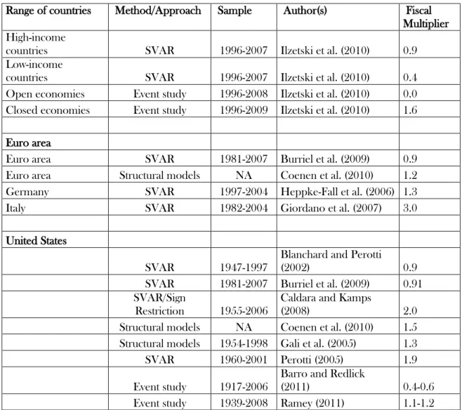
Table 1 summarizes the fiscal multiplier that is estimated according to selected studies. We only present the government spending multiplier because the tax fiscal multiplier is suspected of being biased due to a type of variable error2

. Many studies obtained a fiscal multiplier above 1 for Europe and the USA. However, it is not clear from the theoretical point of view if the fiscal multiplier of emerging and low-income economies should be higher or lower compared to developed countries (Batini et al, 2014). The few available empirical studies suggest that fiscal multipliers in emerging and low-income countries are smaller than in developed countries (Estevão and Samake, 2013; Ilzetski et al, 2013, Ilzetski, 2011, Kraay, 2012).

1 _{The interest rate encompasses expectations of future changes in fiscal policy and can absorb some of the estimated}

effects of fiscal shocks. However, whether the impact of government spending shocks is miscalculated depends on issues such as the autocorrelation structure of the omitted announcement of fiscal policy shock (Perotti, 2005).

2 _{A tax-based fiscal multiplier is generally estimated using tax revenues. The drawback of this variable is the fact that}

tax revenue can change regardless of the policy orientation. In Brazil, for instance, tax revenue has increased over the years even when tax exemptions were intensified, likely because of the formalization process in the labor market. In other words, tax revenue can increase even during expansionary fiscal policies or diminish in times of fiscal austerity.

Table 1 - Some values of the fiscal multiplier in the literature with different methodologies Range of countries Method/Approach Sample Author(s) Fiscal

Multiplier High-income

countries SVAR 1996-2007 Ilzetski et al. (2010) 0.9 Low-income

countries SVAR 1996-2007 Ilzetski et al. (2010) 0.4 Open economies Event study 1996-2008 Ilzetski et al. (2010) 0.0 Closed economies Event study 1996-2009 Ilzetski et al. (2010) 1.6

Euro area

Euro area SVAR 1981-2007 Burriel et al. (2009) 0.9 Euro area Structural models NA Coenen et al. (2010) 1.2 Germany SVAR 1997-2004 Heppke-Fall et al. (2006) 1.3 Italy SVAR 1982-2004 Giordano et al. (2007) 3.0

United States

SVAR 1947-1997

Blanchard and Perotti

(2002) 0.9

SVAR 1981-2007 Burriel et al. (2009) 0.91

SVAR/Sign

Restriction 1955-2006

Caldara and Kamps

(2008) 2.0

Structural models NA Coenen et al. (2010) 1.5 Structural models 1954-1998 Gali et al. (2005) 1.3

SVAR 1960-2001 Perotti (2005) 1.9

Event study 1917-2006

Barro and Redlick

(2011) 0.4-0.6

Event study 1939-2008 Ramey (2011) 1.1-1.2

There have been few studies that estimate fiscal multipliers for Brazil (see table 2). Using the SVAR approach, Peres (2006) obtains small multipliers for the period from 1995 to 2004. Cavalcanti and Silva (2010) use the VAR model, including public debt, as an endogenous variable in the system; their estimate for the multiplier is approximately zero for the period 1995-2008. Based on the signal restriction approach, Mendonça et al. (2009) obtained a negative multiplier for the period 1995-2008. Also using the SVAR approach, Oreng (2012) finds positive and large multipliers using recent data than when using 2004-2011, a period of great macroeconomic stability and low levels of concern regarding debt sustainability. This may have affected the estimation.

Matheson and Pereira (2016) estimate a multiplier of approximately 0.5 using the SVAR approach and controlling for real minimum wage, real primary government spending, and real private credit to the private sector for the 1999-2014 period. However, they noticed that spending and credit public multipliers felt close to zero after the 2008 global crisis. DSGE is also used to estimate the

fiscal multiplier in Brazil as in Celso Junior et al. (2016). The authors obtained a very small but positive government spending fiscal multiplier.

Table 2 – Brazil: some values of the fiscal multiplier

Method Sample Fiscal multiplier Costa Junior et al. (2016) DSGE After 2008 0.055

Matheson and Pereira (2016) SVAR 1999-2014 Close to 0.0 to 0.5 Oreng (2012) SVAR 2004-2011 From 0.7 to 1.0 Mendonça et al. (2009) Sign

restriction

1995-2007 Negative (probability of 77% to GDP contraction)

Cavalcanti and Silva (2009) SVAR 1995-2008 Close to zero Peres (2006) VAR 1994-2005 From 0.3 to 0.4

3. Empirical strategy

Our main goal is to estimate the size of the fiscal multiplier for Brazil — that is, the response of the GDP growth to unexpected shocks of government spending. As is widely known, the value of the coefficient is positively associated with the idea of fiscal policy effectiveness. Usually, one reports peak values in the cumulated impulse response functions (IRF) as the fiscal multiplier.

Our approach can be summarized as seen in figure 1. The first step is to check whether our VAR is a well-specified econometric model by evaluating the residuals tests of normality, autocorrelation, heteroscedasticity, and nonlinearity functional form.

In the second step, we investigate whether the variables and the lags are significant in the estimated models using the Autometrics algorithm3

. Autometrics is an algorithm for automatic model selection within the general-to-specific framework. Autometrics uses one-step and multi-step simplification along multiple paths following a tree search model. Diagnostic tests serve to (additionally) check the simplified models (Doornik and Hendry, 2009). This step is important because a poorly well-specified econometric model cannot provide good estimates for impulse

response functions. With the selection algorithm, we still evaluate the presence of outliers with both impulse and dummy variables.

In the third step, we choose an identification strategy. There are many ways to try to identify the structural shocks. One usual choice is the Cholesky decomposition, but other identification schemes are available. We implement two other identification strategies. The first one is based on Blanchard and Perotti (2002) and Perotti (2005). The second one is the sign-restriction approach. The final step is the IRF (impulse response function) estimation.

Figure 1 - Steps of the empirical strategy

Our VAR models contain two different set of variables. The first set of variables includes net tax revenue (T), government spending (G), and GDP growth (Y), whereas for the second one, we add the inflation rate (π), and money market interest rates known as the Selic rate.

We are aware that VAR models have been subject to several criticisms (IMF, 2010; Romer, 2011; and Caldara and Kamps, 2012). DSGE models are alternative approaches, but they also have drawbacks. We are also aware that other key macroeconomic variables could be taken into consideration, such as trade openness, debt level, and financial market deepening. However, their variations over the time span used in our estimations are negligible. We would strongly recommend including them in cases of a panel-based empirical analysis, as those variables are most likely change across countries. Specification tests/ Autometrics Normality Autocorrelation Homoscedasticity RESET/Nonlinearity Outliers Step 1 Step 2 Step 3 TVAR VAR

3 variables 5 variables _variables3 and 5

Step 4

SVAR SVAR Cholesky

IRF IRF IRF

• Perotti • Sign-restriction • BP

The first identification strategy is to calculate the impulse response function by using Cholesky to decompose the shocks with both the first three and five variables VARs.

The other strategy uses a Structural VAR for the three and five variables system. But first we deal with the case with three variables. The reduced form VAR model is:

𝑋𝑡 = 𝐶(𝐿)𝑋𝑡−1+ 𝑈𝑡 (1)

where 𝑋_𝑡 = [𝑇𝑡 𝐺𝑡 𝑌𝑡]′, 𝐶(𝐿) is an autoregressive lag polynomial and 𝑈𝑡 is the vector of the

reduced form errors.

We can write the reduced-form residuals 𝑈_𝑡 as linear combinations of the structural shocks 𝑉_𝑡 as the following:

𝐴𝑈_𝑡 = 𝐵𝑉_𝑡 (2)

where the matrices A and B describe the instantaneous relations between the reduced form errors and the structural shocks. We cannot identify the matrices A and B without imposing constraints on their elements. A classic method of identification is based on Blanchard and Perotti (2002). We can present the relationship between the reduced form and the structural disturbances of equation (2) in matrix form as follows:

[ 1 0 −𝛼_𝑌𝑇 0 1 −𝛼𝑌𝐺 −𝛼_𝑇𝑌 _−𝛼 𝐺𝑌 1 ] [ 𝑢_𝑡𝑇 𝑢𝑡𝐺 𝑢_𝑡𝑌 ] = [1 𝛽𝐺 𝑇 ₀ 0 1 0 0 0 1 ] [ 𝑣_𝑡𝑇 𝑣𝑡𝐺 𝑣_𝑡𝑌 ] (3)

where the reduced form of the residuals 𝑈_𝑡 = [𝑢_𝑡𝑇 𝑢_𝑡𝐺 𝑢_𝑡𝑌]′, the structural shocks 𝑉_𝑡= [𝑣_𝑡𝑇 _𝑣

𝑡𝐺 𝑣𝑡𝑌]′, and the coefficients 𝛼𝑌𝑇 and 𝛼𝑌𝐺 are respectively the automatic response of economic

activity to net taxes and government spending. 𝛽_𝐺𝑇 measures how the structural shock to the government expenditure contemporaneously affects the tax revenue. Especially for the Brazilian case, unlike Blanchard and Perotti (2002) — BP hereafter — we assume that government decisions on spending are taken before decisions on revenue. Our point is that the Brazilian government decides to spend without considering the possibility of collecting taxes. This implies that 𝛽_𝑇𝐺 _{= 0}4_.

We can write the equations in (3) showing the reduced-form innovations of government spending and revenues:

𝑢_𝑡𝑇 _{= 𝛼} 𝑌𝑇𝑢𝑡𝑌+ 𝛽𝐺𝑇𝑣𝑡𝐺+ 𝑣𝑡𝑇 (4) 𝑢𝑡𝐺 = 𝛼𝑌𝐺𝑢𝑡𝑌+ 𝑣𝑡𝐺 (5) 4 _{BP consider 𝛽} 𝐺𝑇= 0.

Due to the correlation of the reduced-form residuals 𝑢_𝑡𝑗 with structural shocks 𝑣𝑡𝑘, we cannot estimate

𝛼_𝑘𝑗’s using Ordinary Least Squares. Thus, we use exogenous contemporaneous elasticities (𝛼_𝑌𝑇 _and

𝛼_𝑌𝐺_{) to compute the cyclically adjusted reduced-form residuals for net taxes 𝑢}

𝑡𝑇,𝐶𝐴 and for government

spending 𝑢_𝑡𝐺,𝐶𝐴. Then, 𝑢_𝑡𝐺,𝐶𝐴 = 𝑢_𝑡𝐺_{− 𝛼}

𝑌𝐺𝑢𝑡𝑌 = 𝑣𝑡𝐺 (6)

𝑢_𝑡𝑇,𝐶𝐴 = 𝑢_𝑡𝑇_{− 𝛼}

𝑌𝑇𝑢𝑡𝑌 = 𝛽𝐺𝑇𝑣𝑡𝐺+ 𝑣𝑡𝑇 (7)

where we consider the VAR residuals as estimating 𝛽̂. We assume 𝛼_𝐺𝑇 _𝑌𝐺 = 0 because government spending does not respond to real GDP within a quarter following Heppke-Falk et al. (2006). This is in line with BP because they were not able to identify any automatic feedback from economic activity to government purchases of goods and services. We consider various parameter values of 𝛼_𝑌𝑇 according to the literature to analyze a range for the government spending effect on economic growth. Thus, we use the 𝛼_𝑌𝑇 _{values of 0.62, 0.87, 1.54, and 2.08, which are associated respectively with the}

empirical findings for the cases of Spain, Slovenia, European Union (EU), and the United States. The values of these countries/regions are based respectively on the work of Fernández and Cos (2006), Jemec et al. (2013), Burriel et al. (2009) and Blanchard and Perotti (2002). We call the results with the respective 𝛼_𝑌𝑇 values Spain-based, Slovenia-based, European Union-based and BP for the Blanchard and Perotti approach.

Finally, we can estimate the remaining coefficients in the equation for GDP using instrumental variables to take into account the correlation between the regressors and the error term. Following BP, we use cyclically adjusted reduced-form residuals as instruments for the fiscal variables. They may still be correlated with one another, but they are no longer correlated with 𝑣_𝑡𝑌_{. Thus, we can estimate}

𝑢_𝑡𝑌 _{= 𝛼} 𝑇 𝑌_𝑢 𝑡𝑇+ 𝛼𝐺𝑌𝑢𝑡𝐺+ 𝑣𝑡𝑌 (8) using 𝑣̂_𝑡𝑇 _{and 𝑣̂} 𝑡𝐺 as instruments.

In case of the VAR with five variables, we can use the Cholesky decomposition and extend the BP identification strategy for five variables. Perotti (2005) extends his paper to the five-variable framework by including inflation and interest rates in the system, i.e., 𝑋_𝑡 = [𝐺𝑡 𝑌𝑡 𝜋𝑡 𝑇𝑡 𝑖𝑡]′.

We can write the relationship between the reduced-form and structural disturbances in matrix form as for VAR with three variables.

                                                                             i t T t t Y t G t T G i t T t t Y t G t i T i i Y i G T T Y T Y G Y T Y G G v v v v v u u u u u                      1 0 0 0 0 0 1 0 0 0 0 1 0 0 0 0 0 1 0 0 0 0 0 1 1 0 1 0 0 1 0 0 1 0 0 0 1 (9)

The parameter value 𝛼_𝜋𝐺 = −0.5 is our default as well as in other works. We follow Perotti (2005), who argues that the nominal wages of government employees (which represent a large part of government consumption) do not react contemporaneously to changes in inflation. Therefore, the government wage bill decreases in real terms if there is an unanticipated rise in inflation. Again, we assume 𝛼_𝑌𝐺 = 0 and 𝛽_𝑇𝐺 = 0. We also assume 𝛼_𝑖𝐺 = 0 and 𝛼_𝑖𝑇 = 0 like Perotti (2005), which are required to start the procedure. He sets the interest rate elasticities of government spending and net taxes equal to zero, respectively, because interest payments paid and received by the government are excluded from the definition of government spending and net taxes.

Another step of identification strategy consists of adjusting government spending and revenue for the automatic response of these variables to the business cycle and inflation. Therefore, Perotti (2005) regresses individual revenue items on their respective tax base, obtaining an aggregate value for the output elasticity of government revenue (𝛼𝑌𝑇) of 1.85 and an aggregate value for the inflation

elasticity of government revenue (𝛼_𝜋𝑇_{) of 1.25 for the USA. We call this a US-based strategy. As an}

exercise of robustness, we used the values considered by Gnip (2013) for the case of Croatia (𝛼_𝑌𝑇₌

0.92 and 𝛼_𝜋𝑇 _{= 0.73), which is called Croatia-based here}5

. The only difference between the two procedures are the values of 𝛼_𝑌𝑇 _{and 𝛼}

𝜋𝑇 because the identification strategy is the same.

The strategy for the VAR with five variables is similar to the VAR with three variables. Thus, we focus initially on the equations of the reduced-form innovations of government spending and revenues of the matrix-form (9):

𝑢_𝑡𝐺,𝐶𝐴 = 𝑢_𝑡𝐺_{− (𝛼}

𝑌𝐺𝑢𝑡𝑌+ 𝛼𝜋𝐺𝑢𝑡𝜋+ 𝛼𝑖𝐺𝑢𝑡𝑖) = 𝑣𝑡𝐺 (10)

𝑢_𝑡𝑇,𝐶𝐴 = 𝑢𝑡𝑇− (𝛼𝑌𝑇𝑢𝑡𝑌+ 𝛼𝜋𝑇𝑢𝑡𝜋+ 𝛼𝑖𝑇𝑢𝑡𝑖) = 𝛽𝐺𝑇𝑣𝑡𝐺 + 𝑣𝑡𝑇 (11)

Since the structural shocks 𝑣_𝑡𝐺 and 𝑣_𝑡𝑇 are orthogonal, we can use them as instruments to estimate the coefficients.

𝑢_𝑡𝑌 _{= 𝛼} 𝑇 𝑌_𝑢 𝑡𝑇+ 𝛼𝐺𝑌𝑢𝑡𝐺+ 𝑣𝑡𝑌 (12) 5 Perotti (2005) uses 𝛼

𝑌𝑇= 0.94 and 𝛼𝜋𝑇= 0.81 for Australia. These values are close to those considered for Croatia, but

𝑢_𝑡𝜋 _{= 𝛼} 𝑇𝜋𝑢𝑡𝑇+ 𝛼𝐺𝜋𝑢𝑡𝐺 + 𝛼𝑌𝜋𝑢𝑡𝑌+ 𝑣𝑡𝜋 (13) 𝑢_𝑡𝑖 _{= 𝛼} 𝑇 𝑖_𝑢 𝑡𝑇+ 𝛼𝐺𝑖𝑢𝑡𝐺 + 𝛼𝑌𝑖𝑢𝑡𝑌+ 𝛼𝜋𝑖𝑢𝑡𝜋+ 𝑣𝑡𝑖 (14)

With this procedure, we have all the necessary elements to construct the matrices in (9). We next present the sign-restriction approach.

4.2. The sign-restriction approach

We also consider the identification of fiscal policy shocks by sign restrictions on the impulse response. Unlike other approaches used here so far, the sign-restrictions approach does not require the number of shocks to be equal to the number of variables, and this strategy does not impose linear restrictions on the contemporaneous relationship between reduced-form and structural disturbances.

We consider three types of sign restrictions as follows: Caldara and Kamps (2008), Mountford and Uhlig (2009) and a modified version of Mountford and Uhlig (2009). The Caldara and Kamps (2008), here labeled as CK, identify a business cycle shock, a government spending shock and a tax shock. They do not restrict the signal of the monetary policy shock because it is not the focus, and the results of the fiscal policy shock are not sensitive to the non-identification of monetary policy shock. The business cycle shock is identified by the requirement that the impulse responses of output and taxes are positive for at least the four quarters following the shock. The tax shock is identified by the requirement that the impulse responses of taxes are positive for at least the four quarters following the shock, while the government spending requires that the impulse responses of government spending are positive for at least the four quarters following the shock.

Under the Mountford and Uhlig (2009) strategy (MU, hereafter), restrictions are imposed to identify four shocks: a business cycle shock, monetary policy shock, government spending shock and tax shock. In addition to the Caldara and Kamps (2008) strategy, the MU strategy states that the interest rate requires that the impulse responses of interest rate and inflation be positive and negative, respectively, for at least four quarters following the shock. We consider a similar strategy for MU, which is to identify the shocks of inflation and interest rates further, which we call MU_variant. The interest rate requires that the impulse response of interest rate be positive for at least four quarters following the shock. In addition, inflation requires that the impulse responses of inflation rate and interest rate be positive for at least four quarters following the shock.

In line with Uhlig (2005), we write the relationship between the reduced-form disturbances matrix 𝑈_𝑡 and the structural shocks matrix 𝑉_𝑡 as 𝑈_𝑡 = 𝐶𝑉_𝑡 with 𝐸(𝑈_𝑡𝑈_𝑡′) = ∑_𝑢 and 𝐸(𝑉_𝑡𝑉_𝑡′) = 𝐼. Mountford and Uhlig (2005) decompose matrix C into two components for the implementation of the sign-restrictions approach: 𝐶 = 𝑃𝑄, where P is the lower triangular Cholesky factor of ∑_𝑢 and Q is an orthonormal matrix with 𝑄𝑄′_{= 𝐼. The matrix Q is crucial for the sign-restriction approach}

because it collects the identifying weights with each column of Q corresponding to a particular structural shock. We use the penalty function approach to compute the individual elements of Q. The penalty function approach consists of minimizing a criterion function, which penalizes impulse responses violating the sign restrictions. We take 1500 draws from the posterior of the VAR coefficients and the variance-covariance matrix of the reduced-form residuals to identify the structural shocks.

This sign restriction strategy imposes more structure than the Cholesky decomposition and allows us to be relatively “agnostic” of the impact of structural shocks (beyond the contemporaneous effects) (Ellis et al, 2014). This approach also has the advantage of addressing the fiscal anticipated shock and addresses the drawbacks of alternative approaches. This is important because econometricians estimate that fiscal shocks can be anticipated by the private sector to some degree. However, this methodology comes with one problem: the requirement to identify the tax revenue shock makes tax revenues and output not covariate positively in response to the shock, for example. It rules out the output response to revenue shocks (Perotti, 2002).

4.3. Threshold vector autoregressive approach

We now discuss the TVAR (threshold vector autoregressive) approach. Before we present the non-linearity test that indicates whether the presence of non-linearity exists in the equations of the VAR. We use the non-linearity test developed by Castle and Hendry (2010). This is an index test for non-linearity that includes non-linear functions of regressors. Thus, this test analyzes if these functions are important. Consider the regressors 𝑥_𝑡~𝐷_𝑛[𝜇, 𝜎], where 𝜇 is their mean and 𝜎 is their symmetric, positive-definite variance-covariance matrix. We can factorize 𝜎 = 𝐻𝜔𝐻′, where H is the matrix of the eigenvectors of 𝜎 and 𝜔 of the corresponding eigenvalues, such that 𝐻′_{𝐻 = 𝐼. Thus, we use 𝑧}

𝑡=

𝜔1/2_𝐻′(𝑥

𝑡− 𝜇)~𝐷𝑛[0, 𝐼]. For simplicity, consider the following equation:

where 𝑦_𝑡 is the dependent variable and the non-linearity functions are 𝑢_1,𝑡 = 𝑧_𝑡2, 𝑢_2,𝑡 = 𝑧_𝑡3 and 𝑢_3,𝑡 = 𝑧_𝑡𝑒−|𝑧𝑡|_{. Under the null hypothesis,} 𝛿

1 = 𝛿2 = 𝛿3 = 0, and linearity exists. This is an F-test

with 3n degrees of freedom for fixed regressors, where n is the number of observations. The core index test is based on orthogonalized regressors, while the new index test is based on pre-whitened and then orthogonalized regressors.

We consider TVAR as modeling the non-linearity that allows for the possibility of two regimes. The definition of TVAR is

𝑋_𝑡 = 𝑐₁+ ∑𝑃 𝛽_1𝑗𝑋_𝑡−𝑗

𝑗=1 + 𝜗𝑡, 𝐸(𝑣𝑡) = 𝜎1 𝑖𝑓 𝑆𝑡 ≤ 𝑋∗ (16)

𝑋_𝑡 = 𝑐₂+ ∑𝑃 𝛽_2𝑗𝑋_𝑡−𝑗

𝑗=1 + 𝜗𝑡, 𝐸(𝑣𝑡) = 𝜎2 𝑖𝑓 𝑆𝑡> 𝑋∗ (17)

where 𝑆𝑡= 𝑋𝑘,𝑡−𝑑 is the threshold variable from the k-th endogenous variable and d is the delay and

𝑋∗ _{is the threshold. In our application, the threshold variable is the GDP growth. However, we have}

to choose d and 𝑋∗ because they are unknown parameters. We assume a normal prior for 𝑋∗_{~𝑁(𝑋̅, 𝑉̅) where 𝑋̅ = 𝑇}−1_{∑ 𝑋}

𝑡 𝑇

𝑙=1 and 𝑉̅ = 10. We assume a flat prior on the delay d with limits

between 1 and 5. We use the Gibbs sampler that was introduced to simulate the posterior distribution of the unknown parameters and a random walk Metropolis Hasting step to sample 𝑋∗ (Piergiorgio, Mumtaz, 2014, Blake, Mumtaz, 2012). We present the description of the data below.

5. Data Description

Our sample uses Brazilian quarterly data from 1997 to 2014 for a traditional set of variables to address the fiscal multiplier as follows: government spending growth, real GDP growth, net tax revenue growth, money market interest rate growth and inflation rate from the Broad Consumer Price Index (IPCA). We take the first difference of interest rates in the estimation due to non-stationarity of this series, and the growth variables are in a quarter-over-quarter format.

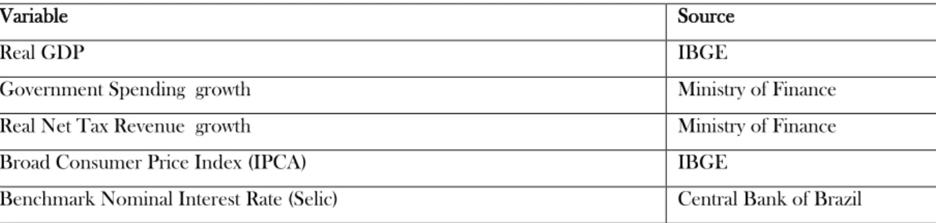
Table 3 shows data and the sources. The data source for interest rates is the Central Bank of Brazil. The real GDP and Broad Consumer Price Index are from the Brazilian Institute of Geography and Statistics (IBGE). The variables government spending and net tax revenue are from the Ministry of Finance.

Table 3. Data descriptions and sources

Variable Source

Real GDP IBGE

Government Spending growth Ministry of Finance

Real Net Tax Revenue growth Ministry of Finance

Broad Consumer Price Index (IPCA) IBGE

Benchmark Nominal Interest Rate (Selic) Central Bank of Brazil

As can be seen, in the case of the Brazil, the longest possible time span results in 72 observations over the course of 18 years, including the last years of a pegged exchange-rate regime (1997-1998). According to Ilzetzki (2011), the more fixed the exchange rate regime is, the larger the fiscal multiplier is. Therefore, our results may be biased when we use the full sample (1997-2014), but a managed floating exchange rate regime is predominant most of the time. In addition, the debt to GDP ratio was mostly very high in comparison to the international standard, which would be biased toward a low multiplier. Throughout the sample, the most remarkable fact is that government spending preponderantly increases.

6. Results

We first discuss the specification tests and then we treat the selection of the model by Autometrics to address potential outliers. We use Autometrics with a significance level of 5% using the block method with the inclusion of impulse indicator saturation (I) and dummy indicator saturation (DI) variables. Table 4 shows the variables selected by Autometrics for the VAR of three and five variables. Besides using variables to control for outliers, this method has Y, G and T lagged respectively on 4, 4 and 2 quarters for VAR with three variables and only selected inflation that is lagged for 1 period for VAR with five variables6

. That is, Autometrics selects the variable of government spending as an explanatory variable only in the VAR with three variables, so it would only obtain a robust non-zero fiscal multiplier in the case with 3 variables by Autometrics7

.

6 _{The algorithm selects, respectively, seven and one dummy and impulse variables.}

7 _{However, if we restrict the criteria so that the significance level is 1%, Autometrics does not select the explanatory}

variable of government spending for VAR with three variables, so the fiscal multiplier is zero. Therefore, our point is that if the fiscal multiplier is not null for Brazil, it is low.

Table 4 – Specification chosen by Autometrics

Three variables Five variables Explanatory variables Y_4 Pi_1

G_4

T_2

Dummy variables DI:1999(1) I:2003(1)

DI:1999(3) DI:1999(4) DI:2002(4) DI:2004(1) DI:2006(4) DI:2009(1) I:2008(4)

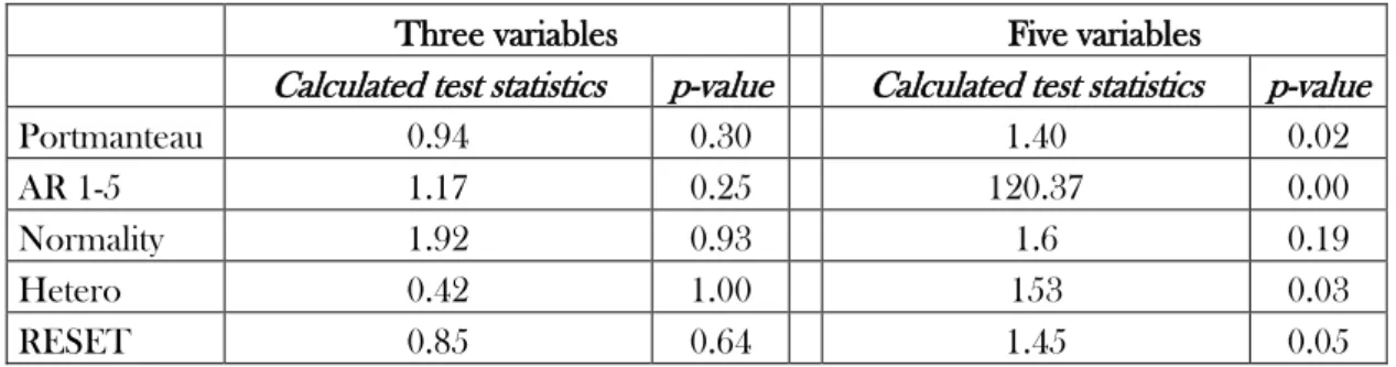
Table 5 shows the specification tests for the selected models discussed above. Our point is that the VAR with five variables is not well specified either by the specification tests or according to the specification suggested by Autometrics. Only the normality test does not reject the null hypothesis of normality for the VAR with five variables. On the other hand, we cannot reject the null hypothesis of all specification tests selected for the VAR with three variables selected by Autometrics. Our more robust model is the one with three variables based on the specification tests.

Table 5 – Specification tests with regression selected by Autometrics

Three variables Five variables

Calculated test statistics p-value Calculated test statistics p-value

Portmanteau 0.94 0.30 1.40 0.02

AR 1-5 1.17 0.25 120.37 0.00

Normality 1.92 0.93 1.6 0.19

Hetero 0.42 1.00 153 0.03

RESET 0.85 0.64 1.45 0.05

Because we can incorrectly detect non-linearity when the data generator process contains outliers, we run a non-linearity test in VAR selected by Autometrics (which selected the specification with outliers) and VAR with full lags (without algorithm selection). We assess the presence of non-linearity in the VAR specifications with full lags. The results are reported in tables 6.1. Both VARs

reject the null hypothesis of linearity at 10% of statistical significance, in which the rejection is stronger for the VAR with five variables. However, the nonlinearity detection in the case of VAR with three variables could be the result of outliers. Now we present the non-linearity test for the VAR selected by Autometrics in table 6.2. The VAR with three variables does not reject the null hypothesis of linearity to 5% of significance, while we can reject this null hypothesis for the VAR with five variables. That is, there appears to be only non-linearity in the case of VAR with five variables. So our best model is the VAR only with three variables and linearity. It appears that we have to move back to the traditional SVAR to infer the effectiveness of fiscal policy in Brazil. Neither monetary policy control (VAR with five variables) nor thresholds and non-linearity (TVAR) should be used in our case. Thus, we estimate the VAR with some form of non-linearity as the next step as robustness.

Table 6.1 - Non-linearity tests on the VARs

New Index Test Core Index Test F statistic p-value F statistic p-value Three variables (G, Y, T) 1.64 0.02 1.44 0.06 Five Variables (G, Y, Pi, T, i) 1.78 0.00 1.63 0.01

Table 6.2 - Non-linearity tests on the VAR selected by Autometrics

New Index Test Core Index Test F statistic p-value F statistic p-value Three variables (G, Y, T) 1.39 0.08 1.05 0.41 Five Variables (G, Y, Pi, T, i) 2.36 0.00 2.05 0.00

We estimate the TVAR to differentiate two regimes when we have a period of low economic growth (which includes periods of crisis) and medium/high economic growth. The threshold of economic growth is slightly higher in the case of TVAR with three variables (1.59% quarter over quarter) compared to five variables (1.12%). In addition, the delay estimated for the threshold variable is three lags in case of three variables and only one in the case of five variables.

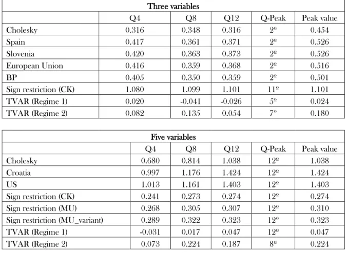
We present the accumulated impulse response function of government spending on economic growth with TVAR in table 7. Basically, our estimates of the models with three or five variables indicate that the fiscal policy has no significant effect on economic growth in periods of low growth (regime 1). Regarding the model with three variables, government spending boosts the economy with a greater effect in the second year with regime 1 or 2. In the case of the model with five variables, government spending has little effect on economic growth initially, which increases considerably in the second year (0.22). As in the identification from the SVAR approach (that we discuss later), the results of TVAR indicate that the peak of the government spending effect on

economic growth is shorter and smaller in the case of three variables in relation to the five variables. The peak of government spending effect on economic growth with TVAR is closer to that with the identification through the sign restriction.

Table 7 - Estimates of the accumulated impulse response functions for different models Three variables

Q4 Q8 Q12 Q-Peak Peak value

Cholesky 0.316 0.348 0.316 2º 0.454 Spain 0.417 0.361 0.371 2º 0.526 Slovenia 0.420 0.363 0.373 2º 0.526 European Union 0.416 0.359 0.368 2º 0.516 BP 0.405 0.350 0.359 2º 0.501 Sign restriction (CK) 1.080 1.099 1.101 11º 1.101 TVAR (Regime 1) 0.020 -0.041 -0.026 5º 0.024 TVAR (Regime 2) 0.082 0.135 0.054 7º 0.180 Five variables

Q4 Q8 Q12 Q-Peak Peak value

Cholesky 0.680 0.814 1.038 12º 1.038

Croatia 0.997 1.176 1.424 12º 1.424

US 1.013 1.161 1.403 12º 1.403

Sign restriction (CK) 0.241 0.273 0.274 12º 0.274 Sign restriction (MU) 0.268 0.305 0.307 12º 0.310 Sign restriction (MU_variant) 0.289 0.322 0.323 12º 0.323

TVAR (Regime 1) -0.031 0.017 0.047 12º 0.047

TVAR (Regime 2) 0.073 0.224 0.187 8º 0.224

We now discuss the VAR results with three and five variables. We choose four and five lags for the VAR with three and five variables, respectively, according to the information criteria. Table 7 shows the estimates of the accumulated impulse response function of economic growth to a 1% change in government spending with different strategies for identification. For instance, consider the Cholesky decomposition as in a VAR with three variables. As we can see, the effect on economic growth are 0.316, 0.348, 0.316, and 0.454 after one year, two years, three years, and at its peak in the second quarter, respectively.

The effects of government spending on GDP growth is greater in the case of using the parameter from Spain (Spain_based) and Slovenia (Slovenia_based), and the greatest effect occurs

within one year — more specifically, in the second quarter8

. However, the peak of government-spending fiscal impact does not vary greatly between different 𝛼s values, even as in the Cholesky decomposition, with a range of 0.45 and 0.53.

It is worth noting the results using signal restriction with three and five variables. As is widely known, another approach to identification is to impose sign restrictions on impulse responses in combination with a criterion function. To run the model with three variables, we follow Caldera and Kamps (2008)’s suggestions because they do not restrict the signal of monetary policy shock, unlike Mountford and Uhlig (2009). The sign-restriction approach does not impose a dogmatic prior on the impact multipliers. This would be our best estimator for the multiplier, especially when we use only three variables. In this case, our estimation for the fiscal multiplier reaches 1.1 in the peak of the impulse response function. However, it is not statistically significant, as shown by the two-standard deviation confidence intervals9

.

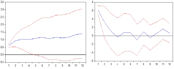
Figure 2 shows an impulse response function that is accumulated (to the left) and instantaneous (on the right) for the GDP growth response to the unexpected shock of government spending as in a VAR with three variables using the parameters for the United States. This indicates that the accumulated impulse response function is different from zero in the first two quarters, while the instantaneous impulse response function indicates that only the effect in the first quarter is statistically significant.

By controlling the monetary policy with five variables by adding the inflation rate and short term interest rate, the effect of government spending on GDP growth is greater only in the third year and no longer in a year, as in the VAR specification with three variables. Additionally, the peak varies in a range between 1.04 and 1.44, as shown in the table. The greatest effect occurs when we consider 𝛼s values using parameters from Croatia, and the lowest effect occurs if we use the Cholesky decomposition10

. This value and the fiscal multiplier behavior are similar to the results of Blanchard and Perotti (2002) for the United States — for example, when the authors obtained a peak of 1.29 in the 15th quarter. Our fiscal multiplier is twice the estimated one by Matheson and Pereira (2016) for Brazil.

8 _{Alternatively, we estimate the models by changing the order of government spending and tax revenue. That is,}

following BP exactly in the case where tax revenue has a contemporaneous effect and is no longer affected by government spending, the result does not change. As an example, the peak of the government spending effect is 0.5263 in this case instead of 0.5258, as we report for the specification using parameters from Spain in Table 7.

9 _{The results are not reported here for convenience; they are available upon request.}

10 _{Alternatively, we change the order between government spending and tax revenue, and the result shows a negligible}

change. For example, the peak is 1.36 instead of 1.37, as we reported in table 5 using the parameter from the US with five variables.

In figure 3, we show the impulse response function that is accumulated (to the left) and instantaneous (on the right) in terms of GDP growth from the government spending unexpected shock according to the VAR with five variables in the US strategy. Figure 3 indicates that the accumulated impulse-response function is different from zero in the first four quarters, while the instantaneous impulse-response function shows that only the effect in the first quarter is statistically significant.

As we can see, the fiscal multiplier increases considerably when the monetary policy is taken into consideration. Generally, the fiscal multipliers are similar regardless of whether the VAR includes the monetary policy. On the other hand, some authors have conducted studies on the impact of the rock-bottom interest rate policy in the US. According to a general New Keynesian model, as explored in Christiano, Eichenbaum and Rebelo (2010), the government spending fiscal multiplier can be larger than usual due to the monetary policy stance. They analyzed a special case of the zero-lower-bound interest rate policy in the US and concluded that this policy amplifies the impact of expansionary stimuli.

Figure 2 – Impulse response function: accumulated (to the left) and instantaneous (on the right) in terms of GDP to government spending shock for the SVAR with three variables with US strategy

Figure 3 – Impulse response function: accumulated (to the left) and instantaneous (on the right) for the SVAR with five variables with US strategy

Therefore, does the monetary policy amplify the fiscal policy in the Brazil case? Literally, as in our empirical findings, the answer would be “yes”. However, our country case is completely different from the case studied by the economic literature when unconventional monetary policy is undertaken. Brazil practices one of the highest and most persistent short-term interest rates in the world, which is caused partially by expansionary fiscal policies11

. According to Auerbach and Gorodnichenko (2012a and 2012b), because the central bank keeps the interest rate high in response to a fiscal expansion defending its inflation targets, this would crowd out private spending and dampen the multiplier. It then appears that there is a sort of puzzle in the relationship between monetary and fiscal policies in Brazil (“the fiscal conundrum”). How could a high short-term interest rate amplify fiscal stimuli? We will attempt to solve such a conundrum with two arguments.

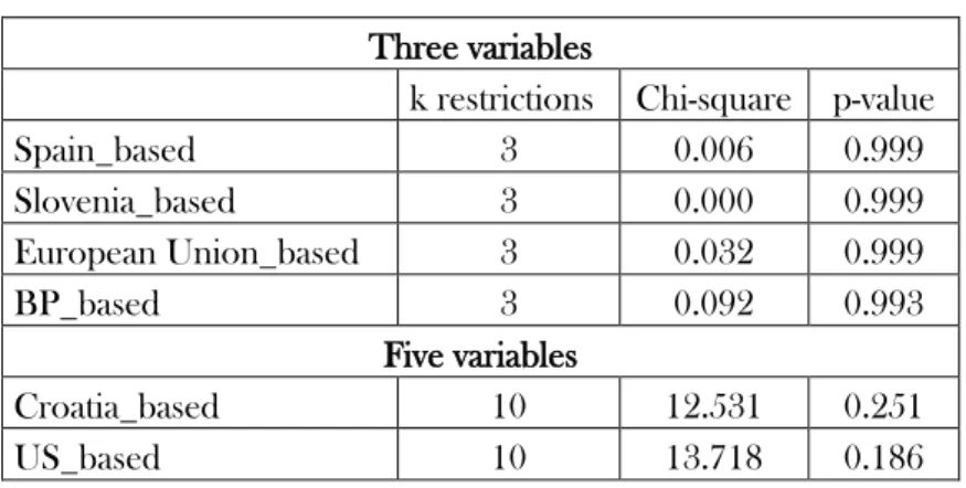
First, the VAR specification with five variables, which includes monetary policy, is far from robust, especially in comparison with the VAR with three variables, as we were able to observe in the specification tests discussed early. We evaluate the SVAR by the likelihood-ratio (LR) test for over-identification, as shown in table 8. We test the k additional restrictions based on the identification strategy. The test statistics follow a chi-square distribution with k degrees of freedom. Under the null hypothesis, the restrictions are valid. According to the table, we cannot reject the null hypothesis in which the restrictions are valid for SVAR with three or five variables. But the p-value is considerably lower for SVAR with five variables.

11 _{In Canzoneri et al. (2002), unexpected shocks of government spending lead to a temporary increase in inflation rate}

Table 8 – LR test for the over-identification of SVAR Three variables

k restrictions Chi-square p-value

Spain_based 3 0.006 0.999 Slovenia_based 3 0.000 0.999 European Union_based 3 0.032 0.999 BP_based 3 0.092 0.993 Five variables Croatia_based 10 12.531 0.251 US_based 10 13.718 0.186

On the other hand, the impact of government spending on real GDP growth is low when we consider the sign restriction. The range of the effect is between 0.274 and 0.323, in line with Mountford and Uhlig (2009). The authors, however, obtained a small fiscal multiplier in four quarters while our findings reached the peak after twelve quarters.

There is a second argument related to the clarification of the monetary-fiscal policy conundrum in Brazil. After all, the response of GDP growth to unexpected shocks in government expenditures double from approximately 0.45 to 1.0 using the full sample and Cholesky approach and from 0.7 to 2.0 using the sample before the 2008 crash. For instance, the short-term interest rate increased from 2009 to 2012, and after a lax cycle, another tight policy stance arose in 2013 until the end of our sample. While fiscal policy was predominantly operating in a countercyclical direction, the monetary policy was operating in a pro-cyclical direction. Besides the lack of robustness issues related the estimation using the monetary policy variable, we do suspect that the level of government spending in percentage of GDP started to put sand in the gears of the fiscal stimulus; it had increased from 14.5% of the GDP to 18.3% and moved quickly to 20% of the GDP.

The risk of solvency tilted as the government spending increased, especially in emerging economies with debt intolerance (Reinhart et al, 2003). According to Gaspar et al. (2016), “high debt constrains fiscal policy, including automatic stabilizers”. Additionally, the Ricardian equivalence can be advocated, in which whatever amount the government overspends today has to be repaid in the future in the form of higher taxes, thus unraveling the government’s efforts to stimulate the economy. However, for emerging market economies like Brazil, the higher the government spending is, the higher the sovereign risk is because the fiscal space evaporates with small amounts of fiscal stimuli. According to the IMF (2015), “the message is loud and clear: governments can use fiscal policy to smooth fluctuations in economic activity, and this can lead to higher medium-term growth”. However, “Fiscal policy also needs to be calibrated to the strength of the recovery without losing sight of debt

sustainability over the medium term”. With increasing government spending, the fiscal policy appears to lose its effectiveness as the fiscal multiplier diminishes. This would be one possible explanation for why a fiscal multiplier appears smaller in the aftermath of the 2008 financial crisis when it was expected to be greater. Fiscal stimuli lost its luster more quickly in commodity-exporting countries such as Brazil than in advanced economies.

We now pose the question of whether the 2008 crisis is making fiscal policy more effective. In this section, we present the results using data up to the third quarter of 2007 to assess whether the crisis of 2008 affected the fiscal multipliers. Empirical exercises using samples after 2008 are not reported here due to the complete lack of robustness, which is mainly due to the degree of confidence. We are then assuming that the comparison between the results using the full sample and the sample for the period prior to the crisis allows us to make inferences about the aftermath of the 2008 crash.

We use the same identification strategies with VAR methodology (SVAR and sign restriction). Table 9 presents the estimates of the accumulated impulse response function of economic growth to a 1% change in government spending with different strategies for identification with the subsample to 2007.

Table 9 - Estimates of the accumulated impulse response functions for different models (until 2007) Three variables

Q4 Q8 Q12 Q-Peak Peak value

Cholesky 0.633 0.713 0.695 5º 0.747 Spain_based 0.627 0.708 0.690 5º 0.742 Slovenia_based 0.633 0.713 0.695 5º 0.746 European Union_based 0.638 0.717 0.699 5º 0.751 BP 0.636 0.713 0,697 5º 0,749 Five variables

Q4 Q8 Q12 Q-Peak Peak value

Cholesky 0.753 1.195 1.791 22º 2.123

Croatia_based 0.720 0.980 1.415 22º 1.584

US_based 0.638 0.896 1.295 22º 1.430

Sign restriction (CK) 0.165 0.187 0.188 13º 0.188 Sign restriction (MU) 0.161 0.180 0.181 13º 0.181 Sign restriction (MUvariant) 0.198 0.219 0.220 11º 0.220

The results from SVAR with three variables show higher government spending effects on real GDP growth before the 2008 crisis compared to the model using our full sample (1997-2014). We

are assuming the fiscal multipliers after 2008 are lower than before the crash, which could be considered counterintuitive. Matheson and Pereira (2016) obtained similar empirical evidence. It appears that countercyclical fiscal policies quickly lose power. We are aware that we have a heavy structure for the data we have available, particularly in the case of reducing the sample to the period before the crisis.

The VAR with five variables, besides its lack of robustness, leads to a greater fiscal multiplier than with three variables. Again, the results indicate that the monetary policy boosts government spending effects on economic growth. In this case, the multiplier is greater for SVAR and Cholesky identification strategies but is lower using the sign restriction identification strategy.

At first glance, it appears that Brazil shows a fiscal conundrum. On one hand, the government spending effect appears to be greater during periods of difficulty than during moderate to high-growth regimes; on the other hand, a high short-term interest rate boosts fiscal multipliers. An inspection in quarterly GDP growth over the sample shows that we are not able to observe different patterns of growth before and after the 2008 crisis. The quarterly real GDP growth is similar between both periods. Difficult periods are not an attribute of the aftermath of the 2008 crisis. However, both real and nominal short-term interest rates are predominantly higher before the 2008 than after, when the fiscal multipliers are greater. This finding is absolutely contrary to the international experience. Ultimately, although the debt to GDP ratio increased in the midst of the 2008 financial turmoil, its trend predominantly declines over the sample. Therefore, the ratios of debt to GDP were higher before 2008, again, when the fiscal multipliers show greater values.

The only way to assess this fiscal conundrum is the tests related to the VAR specifications. As we mentioned previously, the VAR with five variables is not well specified by the specification tests or according to specification suggested by Autometrics. Only the normality test does not reject the null hypothesis of normality for the VAR with five variables. Again, our more robust model is the one with three variables based on the specification tests.

We also attempted to determine the size of the fiscal multiplier before and after the 2008 financial crisis using similar approach to Saxena and Cerra (2008) and Krishnamurthy and Muir (20015). We replaced the variable government spending (G) by the variable G interacted with a dummy variable before the crisis and G interacted with a dummy variable after the crisis, in which the third quarter of 2007 is the threshold for the crisis. We run again the model with three variables using Cholesky approach. Figure 4 shows the impulse response functions for this case.

According the figure 4, fiscal multiplier appears to be higher after the 2008 financial crisis than before it. However, it declines quietly to close to zero. On the other hand, fiscal multiplier appears to

be smaller before the 2008 crisis than after, but remains relatively stable over the time. Over again, fiscal stimuli through government spending underperform to the Brazilian case either before or after the 2008 financial crisis.

Figure 4 – Accumulated impulse response function: before the 2008 crisis (to the left) and after the 2008 crisis (on the right) for the SVAR with three variables and dummy variables with government spending

7. Why is the estimated fiscal multiplier low in Brazil?

Why is the government spending multiplier low in Brazil or even lower than the international experience? First, as highlighted earlier, the public debt level creates a downward bias in the multipliers, while the low degree of the trade openness creates an upward bias. In the United States, the rock-bottom interest rate policy amplifies the multiplier. Conversely, in Brazil, the context of the high interest rate intensifies the impact of government expenditures on GDP growth, although the specifications of the SVAR with monetary policy variables are not robust. When we try to take into account the source of non-linearity, we found outliers masking the findings. Therefore, it is fair to conclude that the fiscal policy is far from effective in the Brazilian case.

Surprisingly, during difficult period of times as after 2008, the fiscal stimuli are less relevant than during good times. Additionally, when controlled by low and high GDP growth according to the TVAR specifications, fiscal multipliers are lower in low growth regimes, although we could not accept the hypothesis of nonlinearity.

-1.0 -0.5 0.0 0.5 1.0 1.5 1 2 3 4 5 6 7 8 9 10 11 12 Accumulated Response of GDPGROWTH to GGROWTHANTES

-1.0 -0.5 0.0 0.5 1.0 1.5 1 2 3 4 5 6 7 8 9 10 11 12 Accumulated Response of GDPGROWTH to GGROWTHDEPOIS

Regardless of positive or negative periods, fiscal spending is predominantly increasing. In nominal terms, from 1997 to 2014, spending increased in 66% of the quarters; in percentage of GDP, 50% of the quarters were expansionary. On average, government spending has increased annually at 0.3% of GDP, 4.8% of GDP of increase in total for the whole time span. Alternately, the government expenditures have increased annually 6% above inflation rate over the time.

Why is there such a resilient increasing trend? First, approximately 90% of the total primary expenditures are not attainable through a retrenchment without changing the Federal Constitution or laws; they are simply mandatory. The remaining 10% are discretionary, although this amount is hard to cut given the risk of paralyzing essential public policies. The pension system represents approximately 40% of total government spending, followed by payroll (21%); among discretionary spending, there are items such as Health, Education and fashionable social programs like Bolsa-Família.

Second, the Brazilian Federal Constitution and several laws govern the allocation of the budgetary resources. In the case of the Federal Administration, it is mandatory to designate at least 18% of the net tax revenue to education and at least 25% in case of States and Municipalities. The Federal Administration and the States and Municipalities must spend at least 12% and 15%, respectively, of their net tax revenue on Health. These rules are important sources of procyclicity in government expenditures.

Likely because of such an institutional framework, as illustrated in figure 5, only 4 out of 18 years show decreases in government expenditures (% of GDP). There is only a single year of decrease in the government spending in the aftermath of the 2008 crisis because there is also one year of decline in spending during the bonanza (2004-2008), also known as the period of super cycle of commodities. The larger shocks in expansions took place after the 2008 crisis, which was from 2008 to 2009 (1.9% of GDP) and from 2011 to 2012 (1.6% of GDP), although large expansions also happened before from 2003 to 2004 (1.4% of GDP). Expansions were rather a rule than an exception during the recent boom in the GDP growth (2004-2008); surprisingly, the more relevant contraction the government spending happened after the 2008 crisis (2011).

From a long-term perspective, there has been a considerable change in government spending since 1997, when the total federal expenditures increased from 13.8% of the GDP to 18.3% of the GDP in 2014 to 19.5% of the GDP, in 2015, a relevant increase in a year of fiscal austerity12

.

Figure 5. Growth of Government Spending (% of GDP) 1997 – 2015

Source: National Treasure Secretariat. Author´s calculation.

Hence, what are the main components of the government expenditure increases over time? First, from 1997 to 2015, primary spending increased to 5.7% of the GDP, while the growth of income transfers to households was approximately 4.0% of the GDP. The pension benefits show the most relevant increase (2.5% of the GDP), followed by elderly/disabled-related benefits, known as LOAS, representing 0.7% of the GDP. Part of the growth of such benefits is related to both the generous eligibility criteria and the public policy stance because they are indexed to the minimum wage corrections. This framework was established in the 1988 Federal Constitution.

As a matter of curiosity, because of this indexation rule, many social benefits increased 78% in real terms over 10 years (2005-2014). At the same time, the number of beneficiaries of the pension system increased by 9 million people, from 23 million to 32 million. Meanwhile, the government decided to enlarge social programs and implement various special (benefits) tax regimes.

Therefore, protected by the Federal Constitution and laws, a combination of a growing number of beneficiaries, a sizable correction in the value of the benefits, and enlarged income transfer programs can be considered relevant factors to explain the upward trend in the government expenditures. In our perspective, the counter-cyclical fiscal policies that were put in practice recently would add some impetus to such tendencies, so the unexpected fiscal shock caused by the government in line with countercyclical policies would influence the output less than expected.

0,9% -0,3% 0,2% 0,8% 0,3% -0,7% 0,5% 0,7% 0,4% 0,1% -0,7% 1,2% 0,8% -1,4% 0,2% 0,4% 1,0% 1,3% -2,0% -1,5% -1,0% -0,5% 0,0% 0,5% 1,0% 1,5% 1998 1999 2000 2001 2002 2003 2004 2005 2006 2007 2008 2009 2010 2011 2012 2013 2014 2015