Intergovernmental grant rules, the "golden rule" of public finance and local expenditures

Carlos Pestana Barros & Nicolas Peypoch

A Comparative Analysis of Productivity Change in Italian and Portuguese Airports

WP 006/2007/DE _________________________________________________________

Paulo Trigo Pereira and João Andrade e Silva

Intergovernmental grant rules, the "golden rule"

of public finance and local expenditures

WP 42/2008/DE/UECE _________________________________________________________

Department of Economics

W

P

ISSN Nº0874-4548

School of Economics and Management

Intergovernmental grant rules, the "golden rule" of public finance and local expenditures

Paulo Trigo Pereira1 and João Andrade e Silva

ISEG – Technical University of Lisbon UECE and CEMAPRE

Rua Miguel Lúpi 20, 1200 Lisboa, PORTUGAL

Abstract

The Stability and Growth Pact and the process of fiscal consolidation in several European countries have enhanced the role of fiscal rules at sub-national level. This paper analyzes the combined effect of a rule to allocate capital and current block grants to local governments and the “golden rule” of public finance (surplus of current balance). We argue that the two fiscal rules introduce significant rigidities and distortions in local governments’ expenditures structure since these mimic the structure of revenues. This effect is particularly relevant in municipalities that are more dependent of intergovernmental grants, mainly rural. On the other hand, urban municipalities with greater tax revenues (current revenues) are constrained in their ability to make capital investments because they receive per capita capital grants below what economies of scale would suggest. An empirical analysis of Portuguese local governments shows that it is no longer the median voter, but fiscal rules, that command the broad pattern of expenditure (current versus capital) at a local level. This paper is a contribution to the literature on the perverse effects of fiscal rules.

JEL Classification: H11, H61, H71, H77

Keywords: Intergovernmental block grants, Fiscal Rules, Local Government Expenditure, “Golden Rule”

1

1. Introduction

The Stability and Growth Pact (SGP) and the process of fiscal consolidation in

several European countries have put some pressure on central governments to impose

fiscal rules at a sub-national level. In fact, since the reference values for both the public

sector deficit and debt refer to general government, i.e. the overall aggregate of public

administrations, any significant slippage on either the deficit or debt of any sub-sector

will have a negative effect on those target values. This seems to be the main argument

behind the spreading of fiscal rules at a sub-national level.

There has been a long theoretical debate concerning the desirability of fiscal

rules. Advocates argue that it is the only way to constrain effectively sub-national

governments in their tendency to increase expenditure and lower taxes, in a growing

spiral of increased deficits and debt, which is a characteristic of electoral incentives in

democracies. In short, given the asymmetric information between voters and their

elected representatives, voting is no longer an effective way to control representatives,

so that some form of fiscal constitution is needed. Fiscal rules are the main elements of

this “constitution”.

Critics of fiscal rules emphasize their perverse effects. They built rigidity in

budgeting and enhance creative accounting because monitored variables apparently

behave well while not observed variables do badly. Fiscal rules do not enable the

smoothing of the economic cycle and constrain the median voter in each jurisdiction

who is no longer the decision-maker in each community.

There was a recent debate on fiscal rules, particularly the “golden rule” (or

surplus of current account), spurred by the need to reform the SGP, which eventually

was reformed in 2005. One debate was whether the fiscal target should continue to be

the overall balance of public administrations (higher than -3% of GDP) or the current

balance. Critics of the overall balance, as a target for fiscal policy, pointed out that

public investments should not be paid totally by current revenues, and that

inter-generational equity suggests that net investment should be financed by borrowing

(Blanchard and Giavazzi 2004 among others). Some critics suggest that the “golden

rule”- even in a modified form - should replace the existing rule of a target for the

overall balance (Creel, J.; Monperrus-Veroni, P. and Saraceno, F. 2007). However,

others point out that although fiscal rules embodied in the Maastricht Treaty and the

should not be introduced into the EMU fiscal framework (Balassone F. and D. Franco

2000).

Turning to the reality of fiscal rules in several countries, most countries have

adopted “domestic stability pacts” in order to set fiscal targets for different tiers of

government (see Sutherland. D.; Price, R. and Joumard, I. 2005 and references herein).

Moreover, the United Kingdom has recently adopted the “golden rule” at national level2

and Germany has established in the Constitution that, in normal circumstances, federal

government borrowing cannot exceed total investment. What does not appear to have

been addressed in the literature is the consequences on local governments patterns of

expenditures of the application of a “golden rule” (for local governments) in the

presence of significant intergovernmental block grants.

This paper aims to contribute to filling this gap through some theoretical and

empirical contributions to the debate looking at two particular fiscal rules. The first rule

(here after rule 1), is the “golden rule” of public finance (surplus of current balance) at

local government level. A corollary of this rule is that any borrowing will not be used to

finance current expenditures but capital expenditures. The second rule (here after rule 2),

is less common but also exists in some countries, either explicitly or implicitly. This is

the constant capital-current ratio of intergovernmental block grants.

The main argument of this paper is that these two rules have a different effect on

sub-national governments with a low and high per capita tax base. Sub-national

governments with low per capita tax base are mainly dependent on intergovernmental

grants, so that the sub-national governments’ broad pattern of expenditure will be

similar to the one imposed by rule 2. Sub-national governments with high per capita tax

bases are much less dependent on intergovernmental grants, and the weight of their own

current revenues (local taxes, fees and other) is significantly higher. Therefore, we

expect a greater variance in the capital-current expenditures’ ratio. However, even

among these municipalities, we predict that net investment is determined mainly by

capital grants independently of economies or diseconomies of scale in local production.

These are some of the perverse effects of excessive fiscal rules.

2

2. Fiscal Rules and the Demise of the Median Voter

Since there are several interpretations of the “golden rule” of public finance (rule

1) it is worth clarifying its meaning in this paper. We will consider that the rule applies

to local governments if they have to comply, on an annual basis, with the balance or

surplus of the current account. The information needed, to impose a “golden rule”, is

that local governments’ accounts enable a clear distinction between current and capital

revenues and expenditures.

Fiscal rule 2, the constant capital-current ratio of intergovernmental block grants

deserves a closer attention. Most intergovernmental grants are formulae based. These

formulae include several variables supposedly reflecting municipal needs (population,

area, special needs associated with the socio-demographic characteristics of population,

and so on). Fiscal rule 2 applies to intergovernmental grant systems that share three

characteristics: (i) most transfers from central government are general transfers, and

thus neither earmarked to specific expenditure categories, nor matched by local

government funds, (ii) transfers for each municipality are calculated through formulae

established in statutes (iii) there is a distinction between current transfers and capital

transfers. Within intergovernmental systems that satisfy these criteria we may

distinguish two cases. The first case is a direct application of fiscal rule 2. A formula

determines the overall amount of grants and the law determines a fixed division of

current and capital grants (e.g. 60% and 40% respectively). Therefore, there is one

formula (or a set of formulae) to define the overall amount of block grants and an

explicit fiscal rule to allocate capital and current grants. The second case is an implicit

fiscal rule 2. There is no fiscal rule to split grants but there are independent formulae,

one for capital grants and a different one for current grants.3 If these formulae, as is

usually the case are a function of relatively stable variables in the short run (such as

population for example) the capital-current grants’ ratio does not change much over

time. An additional argument for the stability of that ratio is that several countries have

“safety net” rules according to which grants received in a given year can not decrease

(or decrease significantly) from previous year grants. There is some difference in the

two cases but we will disregard it in the paper. Our fiscal rule 2, that sets the

capital-current block grants’ ratio encompasses the two situations.

3

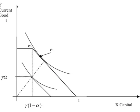
Figure 1 illustrates the effect of fiscal rules 1 and 2 in a limit case of a no tax

base jurisdiction. For simplicity, let us assume that we have just two composite goods, a

current good and a capital good with unitary prices and the maximum amount of the

composite current and capital goods is one. We also assume that borrowing is not

allowed.

Figure 1 Budget constraint under fiscal rules in a low tax base jurisdiction

Under a no fiscal rule regime, we may consider that the preferences of the

median voter will rule so that some allocation in the budget constraint will define a

structure of the budget. Thus if Ui and Uj are the utility functions of the median voters

in municipalities i and j with the same budget constraint, the equilibria levels of

expenditure would be given by points e2 and e1. respectively.

Let us introduce now fiscal rule 2, which states that a given proportion (α) of a

block intergovernmental grant, from central to local governments, is to be accounted as

a “current transfer” and the remaining part (1−α ) as a “capital transfer”.4 These grants

4

As mentioned earlier it is not important whether overall grants are formula based and the proportion of

current block grants is directly defined in statute (as happened in Portugal before 2007), or if current block grants are based in one formula and capital grants are calculated through an independent formula.

X- Capital good. Y

Current Good

1

eo

e1

6 , 0 = α

4 , 0 ) 1

( −α = 1

e2

Ui

are respectively, current and capital expenditures for central government, and current

and capital revenues for local governments.5

If there were no additional rules attached the budget constraint would be the

same as in the no fiscal rule regime.

However, if we introduce fiscal rule 1, of a balanced (or in surplus) current

budget, two main things change. First, we have now a kinked budget constraint. In the

limiting case of a no tax base jurisdiction - where revenues are only from central

governments’ transfers - the kink is precisely at point e0 with coordinates (1−α,α). If

these are the only sources of revenue, e0 is also the balanced current budget allocation.

The further away from e0,the higher is the current budget surplus, and capital budget

deficit (assuming no borrowing). The equilibrium pattern of expenditure will depend on

local preferences. It can be a corner solution (60% current expenditures and 40% capital,

with α=0,6) given by e0, as in municipality i, or any other frontier solution given, for

example, by e1, as in municipality j. Even without borrowing, capital expenditures will

be at least 40% of local expenditures. The kinked budget constraint, produced by fiscal

rules, leads to a decrease in efficiency in municipality i.

Since with these fiscal rules, the budget is balanced at e0, it can be considered a

salientpoint (in Schelling’s (1960) sense), and it is possible to predict that equilibria in

low tax base jurisdictions will tend to concentrate in the neighborhood of e0. Our

hypothesis is that given the importance of the balanced budget concept in public finance,

and some political difficulty in justifying deficits, there will be some tendency for

jurisdictions, with no borrowing, to adapt the structure of expenditures to the structure

of revenues.

The situation is somewhat different in high tax base jurisdictions as illustrated

by figure 2. In these jurisdictions local taxes, fees and other local revenues, are current

revenues, so that the revenue pattern in these local governments has a much smaller

weight of capital revenues. Let us assume that the proportion of intergovernmental

grants on total revenues of the municipality is

γ

(

0

≤

γ

≤

1

)

grants are split in current grants (proportion

α

1

−

α

What is relevant is that there is a current and a capital account and that a proportion (that can be fixed or flexible) of grants goes for each account.

5

The weight of current revenues on total revenues is now

1

−

γ

(

1

−

α

)

α

the previous case. If, for instance, intergovernmental grants represent 30% of total

revenue, with fiscal rule 2 and α=0.6, implies that 88% of total revenues will be current and only 12% capital revenues. Therefore, the current budget would be balanced

if current expenditure is also equal to 88%. Again, the equilibrium expenditure will

depend on local preferences, and the “golden rule” only implies that capital expenditure

cannot be below 12% of the budget. However, any structure of expenditures which

departs dramatically from e3 , will be associated with highly unbalanced current and

capital accounts.

If our Schelling hypothesis is correct we would expect that high tax base

municipalities will have a significant higher proportion of current expenditure and

smaller capital expenditures than low tax base jurisdictions. On the other hand, given

the smaller dependence of intergovernmental grants in high tax base jurisdictions, we

should also expect that the variance of the current expenditures’ weight on total

expenditure would be much larger in these jurisdictions when compared with low tax

base jurisdictions.

Figure 2Budget constraint under fiscal rules in a high tax base jurisdiction

X Capital Y

Current Good 1

e3

e1

γα

) 1 ( α

As argued above, the main aim of this paper is to give empirical evidence, that

the joint effect of fiscal rules 1 and 2 is an inefficient allocation of capital and current

expenditures, mainly in low tax base jurisdictions.

In order to analyze the impact of fiscal rule 1 more accurately, let us assume that

there is no inflation. Let B_t denote local government debt at the end of year t, A_t

borrowing in year t, δ B_t−1 repayment of debt during year t, r the debt implicit interest

rate, C _t current expenditures (excluding debt interests), I _t net investment, T _t taxes,

c t

G current block grants and G_tk capital block grants. The budget constraint of each

municipality is given by:

1

1 −

− + +

+ = + +

+ k _{t t t t t}

t c t

t G G A C rB I B

T δ (1)

On the revenue side the three main sources of income are taxes, intergovernmental

grants and borrowing, on the expenditure side, local governments’ current consumption

plus debt interests, net investment and debt repayment. Let

1

1 −

− = −

− =

∆Bt Bt Bt At δ Bt , i.e. ∆Bt represents the net borrowing of the municipality

during year t. A rearrangement of Equation (1) clarifies the impact of current and capital

balances on net borrowing,

(

) (

)

k t t t c t t

t T G C rB G I

B =− + − − − −

∆ ₋₁ . (2)

A surplus of the budget enables a reduction in local debt. On the other hand, if local

debt does not change, ∆B_t =0, with the “golden rule” of public finance, there must be

a surplus in the current account

(

)

be in deficit ((G_tk −I_t)<0⇔I_t >G_tk). A first conclusion is therefore that, if the debt

remains constant, net local investment has to be greater than intergovernmental capital

grants and the difference is exactly the current surplus since we can rewrite equation (1)

as

(

)

t t t c t t t

t B T G C rB G

I =∆ + + − − ₋₁ + (3)

A second conclusion is that net investment will equal the sum of current surplus,

The usual implication of the “golden rule” is that net borrowing is only to

finance capital formation and not for current expenditures. However, the existence of

capital grants, at the local governments’ level, puts a lower pressure to increase debt.6

A third conclusion is that intergovernmental capital grants can crowd out local

debt. In this case local governments use capital grants to decrease their liabilities. Total

crowding out would mean that debt would decrease by the same amount as capital

grants so that net investment would equal current surplus (see Equation (2)). Partial

crowding out would imply that net investment would exceed current surplus but would

be lower than the sum of the surplus with capital grants.

In order to understand the effect of fiscal rules on local governments we may

consider the extreme and unrealistic case, of a local government without a tax base.7 In

this case:

(

)

∆ =

− c _{t t}

t t k t

t G B G C rB

I (4)

Note that in this case total revenues would be k c

G G

G= + . With no net borrowing, net

investment would have to be greater or equal to capital grants, given the “golden rule”.

If the structure of revenues is 40% capital revenues (grants) and 60% current revenues,

the structure of expenditures could either mimic the structure of revenues, or be

“biased” towards greater capital expenditure.

6

Note that when the “golden rule” is applied to central government, and if revenues from capital grants are not significant (e.g. small grants from the EU to a member state), the implication of the rule is a direct relationship between current surplus, net borrowing and net investment.

7

3. The institutional and financial framework of Portuguese Local

Governments

Portugal is, according to the Constitution, a unitary country with two

autonomous regions (Madeira and Azores), 309 municipalities and around 4000

parishes, the latter with very few competencies. Therefore, our analysis will focus on

municipalities. Although formally a unitary country the financial resources and tax

powers of the autonomous regions are greater than many States (or Lander) in federal

countries. In fact the Constitution (1976) written in the aftermath of the Portuguese

Revolution (April 1974), when there were some threats of regions’ independency

paralleling the independence in former African colonies of 1975, established that the

regions are entitled to all tax revenues (personal and corporate income tax, VAT, excise

taxes, etc.) generated in their territories. Furthermore, the autonomous regions receive

solidarity grants from the State Budget and so do the regions’ municipalities and

mainland municipalities which are, and have been, under the same Local Finance Act

(Lei 2/2007) which establishes criteria for the allocation of current and capital grants

from the State Budget. Formula based intergovernmental grants are the main sources of

financial support to mainland municipalities and any other form of State support is

limited and should be made under a specific contract. However, given the autonomy of

the regions, there has been substantial support to municipalities from the Regional

Government of Madeira. Therefore there is a different treatment of regional and

mainland municipalities, the former receiving grants from three tiers of government (EU,

Portuguese Government and Regional Governments) while the latter only receive from

two tiers (EU and Portuguese Government). In any case the more substantial grants are

from the State Budget.

As in other European countries, the Stability and Growth Pact has enhanced the

adoption of sub-national fiscal rules. In particular a Law was enacted in 2001 (Lei de

Enquadramento Orçamental) in order to define balanced targets for the different

sub-sectors of central government (the State (Estado) and Autonomous Agencies (Fundos e

Serviços Autónomos-FSA)) and social security. The State should have the primary

balance in surplus or equilibrium, the FSA and Social Security should have no deficit.

Later on, the State Budget Laws (from 2003 till 2008) have been establishing that the

Azores) should have no net borrowing requirements, which assuming that there is no

alienation of municipal assets, is tantamount to have the sum of budgets’ surpluses in

one group of municipalities must be at least equal to the sum of budgets’ deficits in the

other group of municipalities. There has been no fiscal rule for regional governments.

Finally, two fiscal rules have been in place for all local governments. Fiscal rule 1, or

the “golden rule” of public finance, which establishes that there should be a surplus in

current budgets. It is a corollary of this rule that any net borrowing is to cover capital

expenditures. Fiscal rule 2, has been embodied in the Local Finance Acts up to 2007.

Overall intergovernmental block grants from the State Budget to municipalities’

budgets are formula based as stated above. After defining the overall amount of grants,

they are split into capital and current grants according to a fixed proportion.

4. Empirical Results

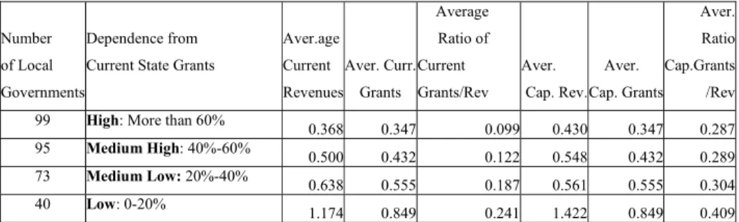
Table 1 shows some 2006 data for Portuguese municipalities. They are sorted out

according to the proportion of central government current grants on municipal current

revenues. It shows that there are 99 municipalities highly dependent on

intergovernmental grants. On average 70% of current revenues and 54% of capital

revenues are grants from central government. These are the low tax base jurisdictions.

Number

of Local

Governments

Dependence from

Current State Grants

Average

Current

Revenue (1000€). Average

Current

Grants (1000€) Average

Ratio Cur

Grants/Rev

Average

Cap. Rev

(1000€).

Average.

Cap. Grants

(1000€)

Average.

Ratio

Cap.Grants

/Rev

99 High: More than 60% 4473.0 3078.5 0.70 4083.6 2052.3 0.54

95 Medium High: 40%-60% 8510.3 4123.4 0.50 5466.6 2748.9 0.55

73 Medium Low: 20%-40% 17608.4 5093.2 0.30 7435.3 3395.5 0.49

40 Low: 0-20% 60221.7 7596.6 0.14 14250.5 5064.4 0.45 Table 1 Average Current and Capital Revenues and Central Government Grants

On the other extreme are local governments where current block grants are smaller than

20% of local revenues. They are simultaneously less dependent from central

government transfers and have a higher average current and capital expenditure. There

is some heterogeneity within each group as shown by coefficients of variation presented

Number

of Local

Governments

Dependence from

Current State Grants

Aver.age

Current

Revenues

Aver. Curr.

Grants

Average

Ratio of

Current

Grants/Rev

Aver.

Cap. Rev. Aver.

Cap. Grants

Aver.

Ratio

Cap.Grants

/Rev

99 High: More than 60%

0.368 0.347 0.099 0.430 0.347 0.287 95 Medium High: 40%-60%

0.500 0.432 0.122 0.548 0.432 0.289 73 Medium Low: 20%-40%

0.638 0.555 0.187 0.561 0.555 0.304 40 Low: 0-20%

1.174 0.849 0.241 1.422 0.849 0.409 Table 2 – Within group coefficients of variation.

As predicted, within group heterogeneity is smaller when the dependence from central

government’s transfers is higher. In highly dependent local governments, current grants

represent, on average, 70% of current revenues and the standard deviation is 10% of that

mean. On the other hand, in local governments with a higher tax base average current

grants represent only 14% of current revenues and standard deviation is 24% of this

value.

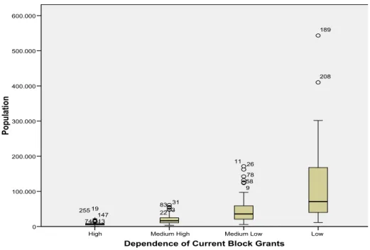
Table 3 adds some information concerning characteristics of each group of local

governments. On average the less populated is the municipality the more dependent it is

from central government grants. Variance within each group also increases with

population.

Dependence of Current Block Grants

Mean

Population Number Std. Deviation

High _{6935.38 99 3448.024}

Medium High _{19636.24 95 12589.840} Medium Low 46344.60 73 37071.725

Low 114607.00 40 110743.425

Total 34265.41 307 55907.092

Table 3 – Population mean and standard deviation

Figure 1 illustrates this with a Box plot where moderate outliers are identified with “o”

and severe outliers with “*”.8

8

Dependence of Current Block Grants Low Medium Low Medium High High P opul at ion 600.000 500.000 400.000 300.000 200.000 100.000 0 19 83 31 22 3 255 147 74 13 208 189 78 58 26 11 9

Figure 3 Municipalities’ dependence on current block grants by population size

No.

of

Local

Govern.

Dependence from

Current State Grants

Average Personal Income Tax per capita (2003) Aver. Current Exp.. (1000€) Average Per Capita Current Expenditure Average. Capital Exp (1000€). Average Per capita Capital Expenditure Aver. Curr. Grants Per capita Aver. Ratio CurrExp/ Capital Exp.

99 High: More than 60% 250.46 4408.1 723.54 3660.4 571.41 505.93 1.55

95 Medium High: 40%-60% 307.16 7578.3 455.38 5525.1 317.94 246.44 1.63

73 Medium Low: 20%-40% 414.08 14639.5 394.86 8960.2 236.76 138.53 1.85

40 Low: 0-20% 722.00 48826.5 499.24 20882.5 222.88 82.83 2.58

Table 4 Average Current and Capital Expenditures and Current/Capital ratio

It is important to note that fiscal rules 1 and 2, do not imply that as the

current-capital revenues’ ratio increase so does the current-current-capital expenditures’ ratio. However,

Table 4 suggests that this happens and this is consistent with our hypothesis. In order to

analyze in more detail this issue we estimated three equations using ordinary least

squares. The first regression relates the expected value of the capital-current

expenditures’ ratio (CCER) with the capital-current revenues’ ratio (CCRR) , the

(POP) of each municipality. To take into account the presence of heteroskedasticity we

used an heteroskedastic consistent procedure to estimate the standard errors (between

parenthesis below the estimated coefficients).

) 10 55 . 0 ( ) 10 84 . 0 ( ) 1064 . 0 ( ) 0641 . 0 ( 10 13 . 0 10 26 . 0 4334 . 0 9288 . 0 1295 . 0 6 8 7 7 ^ − − − − × × × + × + + + −

= i i i i

i CCRR POCR NB POP

CCER 000 . 0 2849 . 95 5579 . 0 ;

307 2 = − = − =

= R F Statistic p value

N

Given the fungibility of resources and the possibility of local governments running

small or large superavits of the current accounts, there should be no reason, a priori, to

believe that the structure of expenditures would mimic the structure of revenues. If local

expenditures were driven by the median voter there should be no statistically significant

relationship between these variables. However, as explained in section 2, the existence

of fiscal rules (the “golden rule” and the rule to allocate grants), introduces a rigidity in

local budgets. Therefore, with fiscal rules we expected that the structure of revenues

(CCRR) command the structure of expenditures (CCER), and this is consistent with the

empirical results. An increase of 0.1 points in the capital-current revenues’ ratio will

originate, ceteris paribus, an increase of 0.093 in the capital-current expenditures’ ratio.

We can also note that an increase in the proportion of own current revenues (i.e. in the

municipalities’ tax base) will originate, ceteris paribus, an increase in the expected

capital-current expenditures’ ratio. Since property related taxes (property tax and a

property transfer tax) are the main local taxes in Portugal, the weight of own current

revenues in total local revenues is linked with property assets. Several municipal capital

expenses are correlated with real estate such as, municipal roads, water and sewage

systems and so on.

The positive coefficient associated with net borrowing underlines that a significant part

of municipalities’ investment is funded by borrowing. Finally, we can verify that,

ceteris paribus, the weight of capital expenditures is slightly higher in more populated

municipalities.

In a second regression, we want to analyze whether net investment per capita

changes with the increasing population size of municipalities. This might be associated

with economies of scale up to a certain threshold of population size. Therefore, the

dependent variable is net investment per capita and the covariates are the population

revenues. For the same reason as before we estimated the standard errors in a

heteroskedastic consistent way.

) 71 . 89 ( ) 10 1015 . 0 ( ) 00043 . 0 ( 6 . 551 10 3352 . 0 001522 . 0 8 . 697 8 2 8 ^ − − × − × + −

= i i i

i POP POP POCR

NIpc 000 . 0 1408 . 58 3653 . 0 ;

307 2 = − = − =

= R F Statistic p value

N

The first comment is that, as expected, we can observe a decrease in net investment per

capita when we move from less populated to more populated municipalities, although at

a diminishing rate. The minimum per capita expenditure is reached around 227

thousand inhabitants, and after that there is an increase in per capita investment. There

are only four municipalities with more than 227.000 inhabitants (Lisbon, Sintra, Porto,

Vila Nova de Gaia). Associated with the overall decrease in net investment, it is

difficult, however, to disentangle what can be explained by economies of scale and

scope and what is a result of fiscal rules and the rigidity of grant design. However,

empirical evidence has shown that economies of scale are strong for small

municipalities and are dependent on the particular local government service. They are

exhausted for a smaller population size for services such as schools and public libraries,

and for a higher population size for services such as waste disposal. Even in this case

where investments are higher, constant returns to scale are reached around 50.000

inhabitants (see Stevens 1978). This suggests that more populated municipalities may

be in a situation of fiscal stress since they receive much less per capita grants than

suggested by economies of scale9.

The second comment is that municipalities with a larger tax base, and consequently a

higher proportion of own current revenues on local revenues, have a lower level of per

capita capital expenses.

This may seem counter-intuitive, but it is not, taking into account the descriptive

statistics presented above. Given that intergovernmental grants more than offset

differences in own local revenues (associated with a lower tax base), municipalities with

more per capita total revenues (including grants, taxes and sales of goods and services)

are those with smaller tax bases. Conversely, municipalities with larger tax yields have

less per capita total revenues.

9

Similar conclusions can be drawn if we regress current expenditures per capita using the same covariates. ) 0 . 139 ( ) 10 1719 . 0 ( ) 00068 . 0 ( 309 . 257 10 7517 . 0 003426 . 0 5 . 754 8 2 8 ^ − − × − × + −

= _{i i i}

i POP POP POCR

CEpc 000 . 0 5348 . 34 2548 . 0 ;

307 2 = − = − =

= R F Statistic p value

N

The relationship between per capita current expenditures and population is similar, and

so it is the turning point (228 thousand inhabitants). Municipalities with a larger tax

base also have a lower level of per capita current expenses. We must note that the

parameter associated with the proportion of own current revenues (POCR) is now

marginally significant (p-value =0.065)

5. Conclusions

Fiscal rules may have some positive implications but also non-intentional negative

effects. This paper emphasizes additional perverse effects of fiscal rules. Apart from the

ones already known in the literature (e.g. incentives for creative accounting), we have

shown that the combination of an intergovernmental grant rule (that allocates capital

and current block grants in a fixed proportion) with the “golden rule” of public finances

(imposing the surplus of the current account) introduces a rigidity in expenditure

structure. Essentially, the ratio of capital-current revenues, which is to a great extent

exogenous to municipalities, has a binding effect on the capital-current expenditures’

ratio. This effect is particularly important in municipalities which are highly dependent

of intergovernmental grants but also in the other local governments.

The rigidity imposed by the fiscal rules has obvious impacts on the inefficiency of

local governments’ decision-making. Moreover, they may create fiscal stress in urban

municipalities, whenever there is a decreasing trend in per capita intergovernmental

grants, and this trend can not be fully explained by the existence of economies of scale.

Intergovernmental block grants in Portugal, as in some other countries, are formula

based. Since the variables underlying these formulae do not change dramatically year

after year, there is some stability in capital and current block grants received by

municipalities, so that the proportion of capital and current grants is also relatively

stable. This shows that the analysis developed in this paper applies to all countries

governments’ revenues, where they are formula based and where there is a distinction

between current and capital grants.

Based on the conclusions of this paper we should expect large inefficiencies at local

government level (e.g. investments above optimal levels in low tax base municipalities)

which can be explained in part by the existence of fiscal rules. This suggests that further

research is needed in this direction. Finally this paper has highlighted some additional

perverse effects of fiscal rules, and suggests that there are, as a consequence of the

Stability and Growth Pact, too much fiscal rules constraining local governments’

behavior.

References

Alesina, A.; Hausman, R., Hommes, R. and Stein, E. 1999, “Budget Institutions and Fiscal Performance in Latin America”, Journal of Development Economics, 59(2): 253-273.

Balassone F. and D. Franco 2000, “Public Investment, the Stability Pact and the ‘Golden Rule’ ”, Fiscal Studies, 21, (2): 207-229.

Blanchard O.J. and F. Giavazzi 2004, “Improving the SGP through a Proper Accounting of Public Investment”, CEPR Discussion Papers 4220.

Creel, J.; Monperrus-Veroni, P. and Saraceno, F.2007,“Has the Golden Rule of Public Finance Made a Difference in the UK ?”, OFCE, Document de Travail nº 2007-13

Dahlberg, M.; Mork, E.; Rattso, J.; and Agren, H. (forthcoming) “Using Discontinous grant rule to identify the effect of grants on local taxes and spending” Journal of Public Economics.

Hallerberg, M.; Strauch, Rolf. and von Hagen, J. 2007, “The Design of Fiscal Rules and Forms of Governance in European Union Countries” European Journal of Political Economy, 23, 338-359

HM Treasury 1997. “A code of Fiscal Stability”, mimeo.

Hogg, R, and Tanis, E. 2001, Probability and Statistical Inference, 6th edition, Prentice- Hall, New Jersey

Milesi-Ferretti, G. M. 2003, “Good, Bad or Ugly? On the Effects of Fiscal Rules with Creative Accounting”, Journal of Public Economics, 88: 377-394

Pereira, P. 1996, “A Politico-Economic Approach to Intergovernmental Lump-sum Grants”, Public Choice, 88: 185-201

Poterba, J. 1995, “Balanced Budget Rules and Fiscal Policy: Evidence from the States”

National Tax Journal, 48 (3): 329-336

Rodden, J. 2002, “The Dilemma of Fiscal Federalism: Grants and Fiscal Performance around the World”, American Journal of Political Science, 46 (3): 670-687

Schelling, T. 1960, The Strategy of Conflict, Harvard University Press, Cambridge MA

Stevens, B. 1978, “Scale, Market Structure and the Cost of Refuse Collection” The Review of Economics and Statistics, 60: 438-448

Sutherland, D.; Price, R. and Joumard, I. 2005, “ Fiscal Rules for Sub-central