(Annals of the Brazilian Academy of Sciences) ISSN 0001-3765
www.scielo.br/aabc
Incorporating electrokinetic effects in the porochemoelastic inclined wellbore formulation and solution
VINH X. NGUYEN1 and YOUNANE N. ABOUSLEIMAN2
1Mewbourne School of Petroleum and Geological Engineering, Poromechanics Institute, The University of Oklahoma
Sarkeys Energy Center, Suite P119, 100 East Boyd Street, Norman, Oklahoma 73019 USA
2Mewbourne School of Petroleum and Geological Engineering, ConocoPhillips School of Geology and Geophysics
School of Civil Engineering and Environmental Science, Poromechanics Institute, The University of Oklahoma Sarkeys Energy Center, Suite P119, 100 East Boyd Street, Norman, Oklahoma 73019 USA
Manuscript received on May 2, 2008; accepted for publication on September 10, 2008
ABSTRACT
The porochemoelectroelastic analytical models and solutions have been used to describe the response of chemically active and electrically charged saturated porous media such as clays, shales, and biological tissues. However, these attempts have been restricted to one-dimensional consolidation problems, which are very limited in practice and not general enough to serve as bench mark solutions for numerical validation. This work summarizes the general linear porochemoelectroelastic formulation and presents the solution of an inclined wellbore drilled in a fluid-saturated chemically active and ionized formation, such as shale, and subjected to a three-dimensional in-situ state of stress. The analytical solution to this geometry incorporates the coupled solid deformation and simultaneous fluid/ion flows induced by the combined influences of pore pressure, chemical potential, and electrical potential gradients under isothermal conditions. The formation pore fluid is modeled as an electrolyte solution comprised of a solvent and one type of dissolved cation and anion. The analytical approach also integrates into the solution the quantitative use of the cation exchange capacity (CEC) commonly obtained from laboratory measurements on shale samples. The results for stresses and pore pressure distributions due to the coupled electrochemical effects are illustrated and plotted in the vicinity of the inclined wellbore and compared with the classical porochemoelastic and poroelastic solutions.
Key words: drilling, electrokinetic, inclined wellbore, osmotic, poromechanics, stability.
INTRODUCTION
It has long been known that chemically active porous media exhibit swelling and shrinking when brought in contact with aqueous solutions. This phenomenon observed in clays, shales, and biological tissues is
Selected paper presented at the IUTAM Symposium on Swelling and Shrinking of Porous Materials: From Colloid Science to Poromechanics – August 06-10 2007, LNCC/MCT.
generally termed osmosis, which is the non-hydraulically driven fluid flow. As such, the coupled fluid flows driven by gradients of chemical and electrical potentials are called chemico-osmosis and electro-osmosis, respectively. Indeed, osmosis through clays and argillaceous rocks has been invoked to explain such observed phenomena as breaching of clay barriers in waste treatment systems (Hudec 1980) and high over pressures in subsurface aquifers (Neuzil 2000). Similarly, osmotic effect is also associated with swelling phenomena observed in charged hydrated biological tissues (Ehlers and Markert 2001). Therefore, the nature of these complex physicochemical interactions requires proper quantification of their effects on the mechanical response of the system.
Of particular interest is the electrochemical effect on the stress and pore pressure distribution in sedi-mentary subsurface where oil and gas exploration activities are being conducted. Osmotic effects may be important in oil fields where clays and shales separate fluid of different salinity and/or electrical potential, especially in wellbore drilling. The electrochemical interactions between the invading drilling fluid with formation pore fluid species and the solid matrix result in changes of pore pressure distribution. Simulta-neously, the effective stress is also modified, which could be detrimental to the formation integrity. Hence, quantitative evaluation and prediction of the overall response require that these coupled interactions be accounted for appropriately.
There is extensive evidence that clay-rich porous formations behave like a semi-permeable membrane, which can restrict solute transport of certain pore fluid species (Young and Low 1965, Olsen 1969, Neuzil 2000). A membrane reflects solutes on the basis of particle size and/or electrical repulsion (Gregor and Gregor 1978). The low permeability and charged surfaces on the constituent clays of shale contribute to its salt rejecting membrane behavior. Differences in chemical potentials of the fluid’s components separated by shale layers cause fluxes of water and solute/ions. Furthermore, when the porous medium, saturated with electrolyte solution, is subjected to an electrical potential gradient, additional electrokinetic effects are introduced. Such electrokinetic effects are associated with the flow of charged particles/ions (streaming currents) and flow of solvent (electro-osmosis) of the pore fluid. In general, these processes involve the coupled and simultaneous flow of fluid, electricity, and chemical species under the influences of mechanical pressure, chemical potential, and electrical potential gradients. Macroscopic transport formulations for these flow phenomena have been derived based on non-equilibrium thermodynamics for irreversible processes (Katchalsky and Curran 1967, Yeung and Mitchell 1993, Malusis and Shackelford 2002, Rosanne et al. 2005).
Early analyses addressing chemical interactions in reactive porous media were presented by lumping the activity-generated osmotic pressure and pore pressure into a chemical potential term, ignoring the solute transport effect (Yew et al. 1990). This chemical potential is treated as a modified pressure, which is used in the evaluation of effective stresses. In other simple approaches, the fluid pressure and solute diffusion effect are taken into account, but ignore the transient coupled deformation-diffusion process (Van Oort 1994).
a plane strain cylindrical wellbore by simplifying the porochemoelastic formulation using the lumped chemical potential mentioned above and ignoring solute transport and electrokinetic effects. Ekbote and Abousleiman (2006) generalized to the fully coupled anisotropic formulation for a chemically active for-mation, and published the analytical solution for the inclined wellbore subjected to in-situ state of stress in isotropic and transversely isotropic formations; however, also neglecting electrical coupling.
Analytical solutions accounting for electrokinetic effects have been limited to the one-dimensional consolidation problem. Esrig (1968) derived such a solution for consolidation with radial drainage due to an electrokinetic application, and pointed out that the rate of pore pressure diffusion was determined by the hydraulic permeability and not by the electrokinetic permeability. His solution, however, employed many simplified assumptions and ignored the ion transport effect. Recently, the full porochemoelectro-elastic one-dimension analytical solutions have been published (Gu et al. 1999, Van Meerveld et al. 2003). These solutions can be applied to limited laboratory and field testing conditions, yet are very restricted and fall short from serving as bench marks for the validation of numerical schemes.
This work presents the analytical porochemoelectroelastic solution to one of the practical field prob-lems: the drilling of an inclined wellbore in a chemically active and ionized shale formation subjected to three-dimensional in-situ state of stress. First, the general isotropic porochemoelastic governing equations extended to incorporate electrokinetic effects are formulated. The inclined wellbore solution is systemati-cally derived in the Laplace transform domain using matrix diagonalization techniques to obtain uncoupled formulations. The obtained solution is used to simulate and study the effects of the coupled electrochem-ical phenomena on stresses and pore pressure distributions in the vicinity of an inclined wellbore, and the subsequent impact on borehole stability.
POROCHEMOELECTROELASTIC GOVERNING EQUATIONS
In a chemically active porous medium, the driving force for the flow of pore fluid and its dissolving species is the chemical potential comprised of the mechanical pressure and osmotic pressure accounting for the chemical activity of pore fluid components. However, the saturating pore fluid is more often an electrolyte solution, which contains solutes that dissolve into electrically charged ions that are sensitive to an electrical potential gradient. On the other hand, many porous media exhibit some degree of ionization, i.e., the solid matrix is electrically charged. For example, the abundant presence of clay minerals such as mont-morillonite, illite, etc., usually renders the shale surface negatively charged due to isomorphic substitution of lower-valence cations for higher valence-cations in the clay structures (Grim 1968). The electrically charged nature of the porous medium generates an electrostatic potential field and, as a result, the move-ment of ionic species is no longer controlled by the chemical potential alone. Incorporating the electrical effect, the total driving force (termed the electrochemical potential) for fluid componentsrunder isothermal condition is expressed as (Katchalsky and Curran 1967)
eμr =Vrp+RTln[ar] +zrFψ =Vrp+RT ln[ζrmr] +zrFψ (1)
whereμr is the electrochemical potential of thert hfluid species (r =solvent, cation and anion),Vr is the partial molar volume,pis the thermodynamic pressure,Ris the universal gas constant,T is the temperature,
ar = ζrmr is the chemical activity,ζr is the chemical activity coefficient, mr is the mole fraction where
P
In an ideal or dilute solution, the activity coefficient has the property that ζr → 1 as mr
→ 0, so that
ar ∼= mr. For simplicity, the pore fluid is modeled as an electrolyte solution comprised of a solvent (f) and one type of dissolved cation(c)and anion(a). The porous solid matrix could be ionized or electrically neutral, but the whole fluid-saturated porous medium is electrically neutral.
TRANSPORTEQUATIONS
Eq. 1 shows that the electrochemical potential difference can be caused by imbalances in the pore pressure, in the chemical composition, or in the electrical potential. The presence of the electrochemical gradient results in simultaneous fluxes of the pore fluid species. For an isothermal aqueous pore solution containing one type of cation and anion, the set of linear phenomenological equations relating the flows and the driving forces in index notation is (Yeung and Mitchell 1993)
qi = L11
∂(−p) ∂xi +
L12
∂(−ψ ) ∂xi +
L13 RT ma o
∂(−ma) ∂xi +
L14 RT mc o
∂(−mc) ∂xi
(2)
Ii = L21
∂(−p) ∂xi +
L22
∂(−ψ ) ∂xi +
L23 RT ma o
∂(−ma) ∂xi +
L24 RT mc o
∂(−mc) ∂xi
(3)
Jia,d = L31
∂(−p) ∂xi +
L32
∂(−ψ ) ∂xi +
L33 RT ma o
∂(−ma) ∂xi +
L34 RT mc o
∂(−mc) ∂xi
(4)
Jic,d = L41
∂(−p) ∂xi +
L42
∂(−ψ ) ∂xi +
L43 RT ma o
∂(−ma) ∂xi +
L44 RT mc o
∂(−mc) ∂xi
(5)
wherexi represents the spatial coordinates, the subscript o denotes initial condition,qi is the total volumet-ric fluid flow vector through the porous medium per unit time (m∙s–1), Ii is the electrical current density (A∙m–2∙s–1),Jia,d ∼= Jia−maqi/V
f
o andJic,d∼= Jic−mcqi/V f
o are the diffusion mass fluxes (mol∙m–2∙s–1) of the ion species relative to that of the water solvent in which Jia andJicare the absolute mass fluxes of the anion and cation relative to the solid framework, respectively.
Lmn are phenomenological coefficients representing various transport processes such as hydraulic conduction (Darcy’s law), electro-osmosis, chemico-osmosis, electrical conduction (Ohm’s law), solute/ion diffusion (Fick’s first law), streaming current and potential, electrophoresis, etc. According to the Onsager principle, these coefficients are related as Lmn = Lnm(m 6= n), which results in only ten independent transport coefficients. These transport coefficients have been well identified in the literature, and can be expressed in terms of familiar field and/or laboratory measurable parameters such as permeability, electro-osmotic permeability, formation resistivity, membrane reflection coefficient, and solute diffusion coefficients as summarized in Table I (Katchalsky and Curran 1967, Yeung and Mitchell 1993, Malusis and Shackelford 2002). The transport coefficients as presented in Table I are modified from parameters as derived by Yeung and Mitchell (1993) to account for the limiting behavior of the effective ion diffusion when the clay membrane behavior is ideal, i.e., the absolute ion fluxes vanish, Jia = Jic = 0, for perfect membrane efficiency,χ =1. Generally, the transport coefficients Lmn are functions of ion concentration. When the system is not too far from equilibrium, i.e., when the macroscopic gradients are sufficiently small, these coefficients can be assumed to be constants. From Table I, modeling of the coupled transport processes requires measurements of only six independent transport parameters{κ, χ , κeo, κe,De f fa ,D
TABLE I
Coupled electrokinetic transport coefficients.
Coefficients Formulas Transport processes
L11 κ+κ
2 eo κe
Hydraulic conduction – Darcy’s law;κ =
k/μis the open circuit(Ii =0)mobility;k is the permeability andμis the fluid viscosity
L12=L21 κeo Electro osmosis/streaming potential κeois the electro-osmosis coefficient L13=L31
−χ κ+(Dae f fzaF/RT)(κeo/κe)
mao/V
f o
Chemical osmosis/streaming current;
L14=L41 −χ κ+(Dce f fzcF/RT)(κeo/κe) mco/V f o
χis the reflection coefficient or membrane efficiency [0,1]
L22 κe
Electrical conduction – Ohm’s law; κeis the electrical conductivity L23=L32 De f fa zaF/RT)(mao/V
f o
Diffusion potential/electrophoresis;
L24=L42 De f fc zcF/RT mco/Vof
F =96500 C/mol is Faraday const.; zaandzcare valences of ions
L33 D
a e f f
RT mao
Vof +
Dae f fzaF
RT mao
Vof 2
/κe+
χmao
Vof 2
κ
Solute diffusion – Fick’s first law
Dae f f =(1−χ )φτDa Dce f f =(1−χ )φτDc
L44 D
c e f f
RT mco
Vof +
Dce f fzcF
RT mco
Vof 2
/κe+
χmco
Vof 2
κ
whereDaandDcare anion and cation diffusion coeff. in free solution;φis porosity;τ is tortuosity
L34=L43
F RT Vof
2
De f fa Dce f fzazcmaomco
κe +
χ
Vof 2
maomcoκ Coupled solute diffusion
CONSTITUTIVEEQUATIONS
In the porochemoelectroelastic constitutive approach, the original Biot’s poroelastic constitutive relations must be extended to account for the electrochemical potentials of all pore fluid solvent and ion species. On a thermodynamic basis, the change in free energy density for a porous medium completely saturated with an electrolyte solution can be expressed as (Coussy 2004)
d W =σi jdεi j −
X
r=a,c,f
Mrdeμr (6)
whereσi j is the total stress tensor,εi j is the linearized strain tensor, andMr is the mass content of the pore fluid species in mole per unit reference bulk volume. The above expression is written assuming infinitesimal deformation and isothermal condition. The electrochemical potentials of all pore fluid components are not independent, but related by the Gibbs-Duhem equation as (Katchalsky and Curran 1967)
−φd p+ X
r=a,c,f
In writing the above equation, it has been assumed that the pore space is completely saturated such that φ = Pr=a,c,f VrMr where φ is the porosity. Application of the Gibbs-Duhem equation into the free energy density leads to
d W =σi jdεi j −φd p (8)
It is obvious that the free energy W admitsεi j and p as state variables instead of the electrochemical potentialseμr of all pore fluid components. As such, the linearized isotropic constitutive equations follow naturally as (Coussy 2004)
dσi j =2Gdεi j+ 2Gν
1−2νdεkkδi j+αd pδi j (9)
dφ = −αdεkk+ 1
Kφd p (10)
whereεkk =ε11+ε22+ε33is the volumetric strain, Gandνare the shear modulus and Poisson ratio,α
is the pore pressure coefficient (PPC), 1/Kφrepresents the pore compressibility,δi j is the Kronecker delta (δi j =1 fori= jandδi j =0 fori 6= j), compression is positive, and repeated index indicates summation. The porosityφ in Eq. 10 can be replaced in favor of the total fluid contentζ using the complete saturation condition and isothermal fluid state equation
dζ = d M sol ρsol
o
= d(φρ sol) ρsol
o
=dφ+φo
dρsol ρsol
o
(11)
dρsol ρsol
o
= K1 f
d p (12)
in which Msol
= Pr=a,c,f Mr is the total fluid mass content (moles) andρsol is the fluid mass density (mole/m3); 1/Kf is the isothermal fluid compressibility. Using Eq. 10 and Eq. 12 into Eq. 11 yields
dζ = −αdεkk+ 1
Md p (13)
where 1/M = 1/Kφ+φo/Kf is the familiar storage coefficient in ground water literature. It is also necessary to obtain the variation of individual fluid component contents by linearizing the relation
dζr = d M r ρsol o
= d(m rMsol) ρsol
o
=mrodζ +φodmr (14)
in whichmr
= Mr/Msolis the mole fraction of fluid species and the initial porosity is related to the initial fluid mass content and density as φo = Mosol/ρosol. Substituting Eq. 13 into Eq. 14 gives the constitutive relations for solute content as
dζr =mro
−αdεkk+ 1
Md p
In summary, the constitutive equations for chemically active and charged saturated porous medium are
dσi j =2Gdεi j + 2Gν
1−2ν δi jdεkk+αδi jd p (16) dζ = −αdεkk+
1
Md p (17)
dζa =mao
−αdεkk+ 1
Md p
+φodma (18)
dζc =mco
−αdεkk+ 1
Md p
+φodmc (19)
Eqs. 16-19 are the same as the original Biot’s poroelastic constitutive formulation without electrochemical interactions. It can be observed that the pore pressure, not the electrochemical potentials, is important; and changing the fluid composition (chemical activity) of the pore fluid and/or electrical potential at constant pressure will not affect the stress, strain and/or total fluid content in the medium. The electrochemical effect, however, enters through the transient nature of the fluid and ion flows due to differences in the electrochemical potentials across the porous medium as shown previously in the transport Eqs. 2-5.
OTHERGOVERNINGEQUATIONS
Other governing equations are the strain-displacement relations (Eq. 20) and conservation equations, which include the quasi-static stress equilibrium equation (Eq. 21), mass balance equations (Eqs. 22-24), and electrical charge conservation equation (Eq. 25) written in index notation as
εi j = 1 2
∂ui ∂xj +
∂uj ∂xi
(20)
∂σi j ∂xi =
0 (21)
∂ζ ∂t = −
∂qi ∂xi
(22)
∂ζa ∂t = −V
f o
∂Jia ∂xi = −
∂ ∂xi
VofJia,d+maqi
(23)
∂ζc ∂t = −V
f o
∂Jc i ∂xi = −
∂ ∂xi
VofJic,d+mcqi
(24)
∂ρe ∂t = −
∂Ii ∂xi
(25)
in whichui is the displacement vector. In the ion mass conservation Eqs. 23-24, the first equality is written by defining the ion volumetric fluxes asqir =VofJir(r =a,c)to be consistent with the previously defined ion contentζr = Mr/ρosol ≈ MrVof. The second equality in Eqs. 23-24 expands the absolute fluxes, Jia andJic, in terms of the relative diffusion fluxes accounting for the advection contributions,maq
In the charge conservation Eq. 25,ρeis the total charge density in the porous medium. It is reasonable to assume an electrostatic condition ∂ρe/∂t = 0, i.e., any electrical charge build-up is instantly equili-brated/neutralized (Sachs and Grodzinsky 1987, Corapcioglu 1991). The charge conservation reduces to (recall Eq. 3)
L12∇2p+L22∇2ψ+L23 RT ma o
∇2ma+L24 RT mc o
∇2mc=0 (26)
where ∇2 is the Laplacian operator. The constitutive Eqs. 16-19, the transport Eqs. 2-5, the
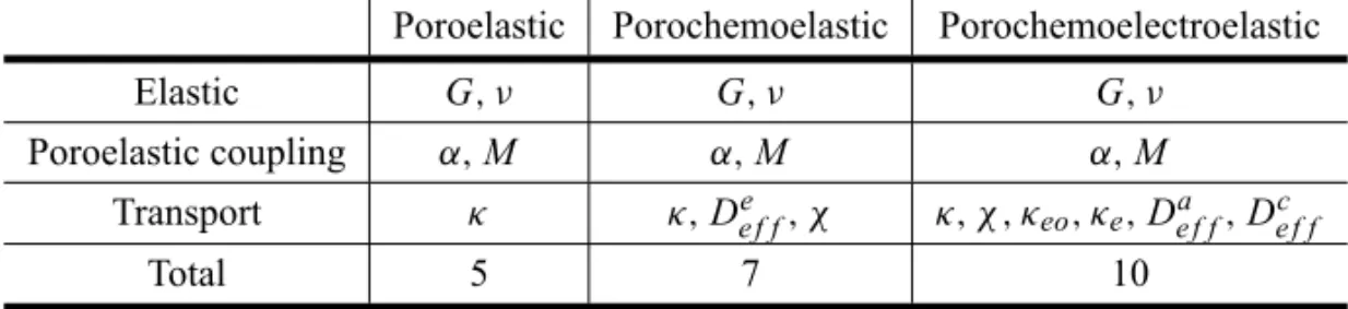
strain-displacement Eq. 20, and the conservation Eqs. 21-26 complete the governing equations for the responses of chemically active and electrically charged porous media saturated with electrolyte pore fluid consisting of two ion species. The porochemoelectroelastic model requires a set of ten independent parameters as opposed to seven by the porochemolelastic and five by the poroelastic models. Table II summarizes and compares the required material coefficients for these models.
TABLE II
Material parameter characterizations for various poromechanics models. Poroelastic Porochemoelastic Porochemoelectroelastic
Elastic G, ν G, ν G, ν
Poroelastic coupling α,M α,M α,M
Transport κ κ,Dee f f, χ κ, χ , κeo, κe,Dae f f,De f fc
Total 5 7 10
FIELD ANDDIFFUSIONEQUATIONS
The governing equations are combined to yield the field and diffusion equations that are used to solve for the coupled stress and pore pressure responses. First, the equilibrium Eq. 21 combined with the stress-strain-pressure Eq. 16 and leads to
∂σi j ∂xi =
2G∂εi j ∂xi +
2Gν 1−2ν
∂εkk ∂xj +
α∂p ∂xj =
0 (27)
Differentiating with respect toxj gives
2G ∂ 2ε
i j ∂xj∂xi +
2Gν 1−2ν
∂2ε
kk ∂xj∂xj +
α ∂
2p
∂xj∂xj =
0 (28)
Taking into account the strain-displacement Eq. 20, the following relation can be derived
∂2ε
i j ∂xj∂xi =
1 2
∂2
∂xj∂xi
∂u
i ∂xj +
∂uj ∂xi
= ∂
2
∂xj∂xj
∂u
i ∂xi
= ∂
2ε
kk ∂xj∂xj ≡ ∇
2
εkk (29)
Using Eq. 29, Eq. 28 is simplified to the field compatibility equation in poroelasticity (Rice and Cleary 1976)
∇2
εkk+ η Gp
=0 (30)
The diffusion equations are derived by substituting the fluid/ion content constitutive Eqs. 17-19 and the transport Eqs. 2-5 into the mass balance equations Eqs. 22-24 as
−α∂εkk ∂t +
1
M ∂p
∂t =L11∇ 2p
+L12∇2ψ+L13 RT ma o
∇2ma+L14 RT
mc o
∇2mc (31)
mao
−α∂εkk ∂t +
1
M ∂p
∂t
+φo ∂ma
∂t
=Vof
L31∇2p+L32∇2ψ+L33 RT ma o
∇2ma+L34 RT
mc o
∇2mc
+mao∂qi ∂xi +
qi ∂ma
∂xi
(32)
mco
−α∂εkk ∂t +
1
M ∂p
∂t
+φo ∂mc
∂t
=Vof
L41∇2p+L42∇2ψ+L43 RT ma o
∇2ma+L44 RT mc o
∇2mc
+mco∂qi ∂xi +
qi ∂mc
∂xi
(33)
The last terms on the right-hand side of Eqs. 32-33 correspond to ion transport by advection. When the hydraulic diffusion(κ)is smaller than the effective ion diffusion(De f fr Vof/RT), the ion transport process is dominated by the diffusion mechanism (Yeung and Datla 1995). As a result, the advectionqi(∂mr/∂xi) terms in Eqs. 32-33 can be neglected, leading to complete linearization of the ion transport equations. Furthermore, the assumption of electrostatic condition allows us to conveniently uncouple the pressure and ion concentrations from the electrical potential field. Application of the Poisson-type Eq. 26 into the diffusion Eqs. 31-33 to eliminate the electrical potential and grouping like terms yields
−α∂εkk ∂t +
1
M ∂p
∂t =D11∂ 2p
+D12∂2pa+D13∂2pc (34)
mao
−α∂εkk ∂t +
1
M ∂p
∂t
+ φoV f o
RT ∂pa
∂t = D21∇ 2
p+D22∇2pa+D23∇2pc (35)
mco
−α∂εkk ∂t +
1
M ∂p
∂t
+φoV f o
RT ∂pc
∂t =D31∇ 2p
+D32∇2pa+D33∇2pc (36)
wherepa
=(RT/Vof)maandpc =(RT/V f
o )mcare pressure equivalent terms andDklis a non symmetric lumped coefficient matrix defined in terms of the original transport coefficientsLmnand is given as
D11 D12 D13 D21 D22 D23 D31 D32 D33
=
κ −χ κ −χ κ
mao(1−χ )κ De f fa Vof/RT
−mao(1−χ )χ κ −mao(1−χ )χ κ
mco(1−χ )κ −mco(1−χ )χ κ De f fc Vof/RT
−mco(1−χ )χ κ
(37)
electro-osmotic permeability and electrical conductivity. The effective transport coefficients Dklare, how-ever, dependent upon the electrostatic potential field internal to the charged shale, i.e., function of fixed charge density in the shale solid matrix and ion concentration in the shale pore fluid. Thus, the significant contribution of an externally applied electrical field may only manifest as possible boundary condition ef-fect, e.g., flux boundary condition. The electrical transport coefficients do come into play when calculating the flux or the streaming potential field established under perturbed conditions. This observation has been confirmed by laboratory and field data as reported by Esrig (1968). In the following section, the set of governing field Eqs. 30 and 34-36 will be applied to model the drilling of an inclined wellbore through a chemically active and ionized shale formation.
INCLINED WELLBORE SOLUTION
The inclined wellbore problem assumes that the wellbore axis generator is deviated with respect to the far field in-situ state of stresses, SH, Sh, and SV as shown in Fig. 1(a). The deviation is defined by the inclination angle, ϕz, formed with the vertical direction, and the azimuth angle, ϕy, formed with maxi-mum horizontal in-situ stress. The porochemoelastic analytical solution for an inclined wellbore drilled in chemically active rock formations has been published by Ekbote and Abousleiman (2006). Their solu-tion approach follows the loading decomposisolu-tion scheme as in Cui et al. (1997) to arrive at the final three-dimension solution. By the same token, the approach is applicable to the current linear porochemo-electroelastic model with the relevant initial and boundary conditions for the stress, pore pressure, ion concentrations, and electrical potential.
(a) (b)
Fig. 1 – (a) Schematic of an inclined wellbore; (b) Far-field stresses, pore pressure and ion concentrations in thex yzlocal wellbore coordinate system.
INITIALEQUILIBRIUMCONDITIONS
(a) (b)
Fig. 2 – (a) Initial state before drilling; (b) After drilling of wellbore.
formations, e.g., shale, is not electrically neutral as depicted in Fig. 2(a). It contains excess exchangeable cation concentration to counter-balance the negative fixed charges on the shale layers according to the electrical neutrality requirement as
zcmco+zamoa+zf cmof c=0 (38) wherezc>0 andza,zf c<0 are the valences of the cation, anion and shale fixed charge, respectively, and
mf cis the concentration of these fixed charges on the surface of the solid shale matrix expressed in terms of mole fraction. Calculation of the initial ion concentration in the pore fluid requires knowledge of the pore water activity of the formation, e.g., measured by an osmometer. The measured pore water activity is actually the water activity of a free outer solution that is in thermodynamic equilibrium with the formation initial state which requires equality of individual electrochemical potentials (Overbeek 1956)
e
μeqf =eμof; eμceq =eμco; eμaeq =eμao (39) For a solution containing electro neutral salt, CxAy, which dissociates into x cations of type C having valencezcandyanions of type A having valenceza, the measured water activity can be used to estimate the equilibrium outer salt concentration,ms
eq, through the relationa f o =ζ
f eqm
f
eq ∼=1−(x+y)mseq assuming dilute solution(ms
eq ≪1). On the basis of Eqs. 1 and 39, we may write for the equilibrium case
Vofpeq+RT ln[1−(x+y)mseq] =V f
o po+RT ln[1−(mao+m c
o)] (40)
Vocpeq+RTln[xmseq] +z c
Fψeq =Vocpo+RT ln[mco] +z c
Fψo (41)
Voapeq+RTln[ymseq] +z aFψ
eq =Voapo+RTln[mao] +z aFψ
o (42) Making use of the electro neutrality condition,x zc+yza =0, for the outer solution, the electrical potential term is eliminated by multiplying Eq. 41 with x and Eq. 42 with y, and adding the resultant equations together to arrive at
(mco)x(mao)y =(xmseq)x(ymseq)yexp
x Vc o +yVoa
RT (peq−po)
∼
=xxyy(mseq)x+y (43)
VN a+
o =2.33e-6 m3/mol, andVoCl−=15.17e-6 m3/mol, then, the termRT/(x Voc+yVoa)is approximately 146 MPa, which is usually two orders of magnitude greater than the pressure difference. For brevity, only the results for x: y ≡1:1 salts such as NaCl and KCl are presented in the following. Derivation for salt solution of differentx: ycan be carried out analogously. Eq. 43 simplifies to
mcomao=(mseq)2 (44)
Solving Eq. 44 together with the electro neutrality requirement inside the formation (Eq. 38) for the initial ion concentrations gives
mao =(0.5/za)
−zf cmf c−q(zf cmf c)2
−4zazc(ms eq)2
(45)
mco=(0.5/z c
)−zf cmf c+ q
(zf cmf c)2
−4zazc(ms eq)2
(46)
To complete the calculation of initial ion mole fraction, the amount of negative fixed charge must be estimated. The fixed charge mole fraction is related to the formation Cation Exchange Capacity (CEC) measured in milli-equivalent of cations per 100 grams of dry clay by
mf c=10∗C EC(1−φo)ρsVof/φo (47)
in whichρs is the average grain density in g/cc andVof is the water molar volume in liter/mol. Assuming
zc
= 1 and za = zf c
= −1, and expressing the fixed charge concentration in terms of CEC and the equilibrium salt salinity in terms of measured water activity, the initial anion concentration in the formation is (Hanshaw 1964)
mao =0.5
−10∗C EC(1−φo)ρsVof/φo+
q
[10∗C EC(1−φo)ρsV f
o /φo]2+(1−a f o)2
(48)
Examination of Eq. 48 shows that, for two formations of the same porosity, the one with the higher sur-face charge density or CEC will accommodate fewer anions and, thus, expulse more free salt. Hence, a smectite abundant formation (CEC ∼ 80-120 meq./100gr) exhibits more reactivity and more ideal membrane behavior with aqueous solution than an illite formation (CEC ∼ 20-30 meq./100gr). Mean-while, as the porosity tends toward zero, ma
o vanishes, implying that the more compacted the formation, the more efficient is the shale’s ion exclusion behavior. It is also interesting to see that when the measured pore water activity is high, e.g.,aof →1,maoapproaches zero. However, this does not necessarily mean that all the anions are excluded from the formation since the pore fluid could simply be just water(awfater =1).
BOUNDARYCONDITIONS
continuous or else there would be infinite fluxes across the boundary. This leads to similar thermodynamic requirements as in Eq. 39
e
μmudf =eμshalef r
=Rw; eμ
a
mud =eμ a shale
r
=Rw; eμ
c
mud =eμ c shale
r
=Rw (49)
whereRwis the wellbore radius. Following a similar procedure and replacing the corresponding subscripts “eq” and “o” with “mud” and “r = Rw”, the ion concentrations in the shale at the wellbore wall are determined as
mashaler
=Rw =0.5
−mf c+ q
(mf c)2+4(ms mud)2
(50)
mcshaler
=Rw =0.5
+mf c+ q
(mf c)2+4(ms mud)2
(51)
Eqs. 50-51 reveal that the total ion mole fraction in the formation at the boundaryma o
r=Rw+m
c o
r=Rw = p
(mf c)2+4(ms
mud)2is larger than or equal to the outer mud ion concentration of 2msmud. Consequently, there exists a fixed-charge-induced osmotic pressure differential at the wellbore mud/shale interface ac-cording to
pshale
r=Rw−pmud = RT/V
f o
∗ mashaler
=Rw+m
c shale
r=Rw−2m
s mud
= RT/Vof∗ q
(mf c)2
+4(msmud)2
−2msmud
(52)
The above induced osmotic pressure is calculated based on the requirement of continuous electrochemical potential of the electrically neutral water at the borehole wall,eμmudf =eμshalef r
=Rwin Eq. 49. Additionally,
Eq. 52 shows that for the same drilling mud salinity, the higher the CEC of the formation, the larger the osmotic pressure differential developed at the wellbore wall. When the formation is free of fixed charge, i.e., CEC,mf c
→ 0, the pressure and ion concentrations are indeed continuous at the boundary:
pshale
r=Rw = pmud and m
a shale
r=Rw = m
c shale
r=Rw = m
s
mud. The discontinuities of ion concentrations and pore pressure at the mud/shale interface are well known in chemistry as the Donnan equilibrium effect (Overbeek 1956).
Accordingly, the boundary conditions to be imposed at the wellbore wall,r = Rw, are
σrr = σm +σdcos[2(θ −θr)]
H[−t] +pmudH[t] (53) τrθ = −σdsin[2(θ −θr)]H[−t] (54) τr z = Sx zcos[θ] +Syxsin[θ]
H[−t] (55)
p = poH[−t] + pmud+1pmud/shale
H[t] (56)
pa= RT/Vof maoH[−t] +(msmud+1mamud/shale)H[t] (57)
And at the far field,r → ∞
σx x =Sx; σyy =Sy; σzz =Sz (59)
τx y = Sx y; τyz = Syz; τx z =Sx z (60)
p= po; pc =(RT/Vof)m c o; p
a
=(RT/Vof)mao (61)
In the above,σm,σd,θr are parts of the stress boundary condition and rotation angle in polar coordinate for a circular borehole as defined in Cui et al. (1997)
σm =(Sx +Sy)/2 (62)
σd =0.5
q
(Sx−Sy)2+4S2x y (63)
θr =0.5 tan−1[2Sx y/(Sx −Sy)] (64)
wheret is time and H[t] is the Heaviside unit step function (H[t < 0] = 0 and H[t ≥ 0] = 1). Sx, Sy,
Sz,Sx y,Sx z, andSyz are far-fieldin-situstresses transformed into the local wellbore coordinate(x,y,z)as depicted in Fig. 1(b). 1pmud/shale, 1mcmud/shale and1m
a
mud/shale are the pressure and ion concentration differential at the mud/shale boundary defined as
1pmud/shale = pshale
r
=Rw−pmud (65)
1mamud/shale =mashaler
=Rw−m
s
mud (66)
1mcmud/shale =mcshaler
=Rw−m
s
mud (67)
wherema shale
r=Rw, m
c shale
r=Rw, and pshale
r=Rw are defined in Eqs. 50-52. It should be noted here that
since the governing field and diffusion equations are uncoupled with the electrical potential field and the boundary conditions are of Dirichlet’s type, i.e., the values of the variables are specified on the problem’s boundaries, it is not necessary to specify the boundary condition for the electrical potential field, unless we want to solve for the fluxes and/or streaming electrical potential field.
THEPROBLEMSOLUTIONS
Following Cui et al. (1997), the problem can be solved by the superposition of three sub-problems. The three sub-problems are described as the modified plane strain problem, the uniaxial problem, and an anti-plane shear problem. It was shown that, of the three problems, solutions for the uniaxial and anti-anti-plane shear problems are purely elastic since they do not generate excess pore pressure (Cui et al. 1997). The solutions to the individual problems are presented here.
Problem 1: plane strain problem
At the far field(r → ∞)
σx x =Sx; σyy= Sy;σzz=2νσm +α(1−2ν)po (68)
τx y =Sx y; τyz =0; τx z =0 (69)
p= po; pc= RT/Vof
mco; pa = RT/Vofmao (70) At the wellbore wall(r = Rw)
σrr =(σm +σdcos[2(θ −θr)])H[−t] + pmudH[t] (71) τrθ = −σdsin[2(θ −θr)]H[−t] (72)
p = poH[−t] + pmud+1pmud/shale
H[t] (73)
pa= RT/Vof maoH[−t] +(msmud+1mamud/shale)H[t] (74)
pc = RT/Vof
mcoH[−t] +(msmud+1mcmud/shale)H[t] (75) The boundary conditions of this problem are designed such that a plane strain solution can be used. First, a reduced set of the governing Eq. 30 and Eqs. 34-36 is derived to obtain the time-dependent solutions for a plane strain condition. Specifically, the field Eq. 30 is rewritten in polar coordinate(r, θ )as
∂2 ∂r2+
1
r ∂ ∂r +
1
r2
∂2
∂θ2 εkk+
η Gp
=0 (76)
Based on the boundary loading conditions Eqs. 71-75, the various variables can be decomposed as (Carter and Booker 1982)
p,pa,pc, εkk, σkk, σrr, σθ θ =
P,Pa,Pc,Ekk,Skk,Srr,Sθ θ cos(nθ ) (77)
τrθ =Trθsin(nθ ) (78)
where P, Pa, Pc, Ekk, S
kk, Srr, Sθ θ, and Trθ are functions of time and radial distance only, andn is an
integer number depending on loading conditions. To facilitate the Laplace transform technique, we solve for the perturbations/changes with respect to the initial reference state, so that the initial conditions and far field boundary conditions for all variables vanish identically.
Incorporating Eq. 77 into Eq. 76 to eliminateθ dependency and seeking bounded solutions gives
e
Ekk = −(η/G)Pe+Cor−n (79) whereCo=Co[s]is a constant to be determined from boundary conditions, the tilde sign∼denotes Laplace transform solution and s is the Laplace variable. Utilizing Eq. 79 to replace the volumetric strain in the diffusion Eqs. 34-36 leads to
s 1 M + αη
G 0 0
mao M1 +αηG φoVof
RT 0 mc o 1 M + αη G
0 φoVof
RT
| {z }
[Y]
e P e Pa e Pc =
D11 D12 D13
D21 D22 D23 D31 D32 D33
| {z }
[D]
∇n2
e P e Pa e Pc +α 1
ma0 mc 0
where ∇2
n = ∂2/∂r2+(1/r)(∂/∂r) −n2/r2. The above system of differential equations only yields realistic solutions if the 3×3 coefficient matrix[Z] = [Y]−1[D]is positive definite. It is easy to verify that[Z]is positive definite since all determinants of[Z]and its leading principal sub matrices are positive (Johnson 1970).
The solution to this coupled system can be found by uncoupling the diffusion equations using matrix diagonalization techniques (Farlow 1993). Here, the general solutions are straightforward and given by superimposing the homogenous solution and the particular solution as
e
P =Cof1r−n+m11C1Kn[ξ1r] +m12C2Kn[ξ2r] +m13C3Kn[ξ3r] (81) e
Pa =Cof2r−n+m21C1Kn[ξ1r] +m22C2Kn[ξ2r] +m23C3Kn[ξ3r] (82) e
Pc =Cof3r−n+m31C1Kn[ξ1r] +m32C2Kn[ξ2r] +m33C3Kn[ξ3r] (83)
where Ci = Ci[s] are constants to be determined from the boundary condition, Kn[ξir] is the modified Bessel function of the second kind of order n, ξi = √s/λi, in which λi is the eigenvalue of [Z] with {m1i,m2i,m3i}as its corresponding eigenvector, and fi =α[Y]−1{1ma0 mc0}T fori =1,2,3.
Once the pressure solutions are obtained, the general solutions for stress, strain, and displacement are straightforward to obtain using the constitutive equations (Eq. 16) and strain-displacement relations (Eq. 20). For brevity, these derivations are not presented here. To determine the constants Ci, the bound-ary conditions for this problem are further decomposed into three loading cases namely: elastic radial loading, diffusion, and a poroelastic deviatoric stress loading case.
• Case 1
The boundary conditions at the wellbore wall are
σrr = −σm+pmud; σrθ =0; p= pa= pc =0 (84)
and the solution is purely elastic as given by the classical Lamé solution
σrr(1) = −(σm −pmud)(Rw2/r
2) (85)
σθ θ(1) =(σm−pmud)(R2w/r
2) (86)
where the superscript (1) denotes the loading case and only the non-zero solutions are listed.
• Case 2
The boundary conditions at the wellbore wall are
σrr =σrθ =0; p=1p; pa =1pa; pc=1pc (87)
domain using the Stehfest’s algorithm (Stehfest 1970) as presented in Appendix A
sep(2)=m11118[ξ1] +m12128[ξ2] +m13138[ξ3] (88)
sepa(2) =m21118[ξ1] +m22128[ξ2] +m23138[ξ3] (89) sepc(2)=m31118[ξ1] +m32128[ξ2] +m33138[ξ3] (90) seσrr(2)= −2η{m11114[ξ1] +m12124[ξ2] +m13134[ξ3]} (91) seσθ θ(2) =2η
m1111(4[ξ1] +8[ξ1])+m1212(4[ξ2] +8[ξ2])+m1313(4[ξ3] +8[ξ3]) (92)
where the tilde∼denotes the quantities in the Laplace transform domain. In the above
11=
(m22m33−m23m32)1p+(m13m32−m12m33)1pa+(m12m23−m13m22)1pc
/m (93)
12=
(m23m31−m21m33)1p+(m11m33−m13m31)1pa+(m13m21−m11m23)1pc
/m (94)
13=
(m21m32−m22m31)1p+(m12m31−m11m32)1pa+(m11m22−m12m21)1pc
/m (95)
m=m11(m22m33−m23m32)−m12(m21m33−m23m31)+m13(m21m32−m22m31) (96)
1p= pmud+1pmud/shale−po (97) 1pa= RT/Vof msmud+1mamud/shale−mao (98) 1pc= RT/Vof msmud+1mcmud/shale−mco (99) 8and4are functions defined as
8[x] =Ko[xr]/Ko[x Rw] (100)
4[x] =K1[xr]/(xrKo[x Rw])−RwK1[x Rw]/(xr2Ko[x Rw]) (101)
• Case 3
The boundary conditions at the wellbore wall are
σrr = −σdcos[2(θ −θr)]; σrθ =σdsin[2(θ−θr)]; p = pa = pc=0 (102) and the solutions in Laplace transform domain are
sep(3)=σd
m11D1K2[ξ1r] +m12D2K2[ξ2r] +m13D3K2[ξ3r] +D4f1(Rw2/r 2) cos
[2(θ −θr)] (103)
sepa(3)=σd
m21D1K2[ξ1r] +m22D2K2[ξ2r] +m23D3K2[ξ3r] +D4f2(Rw2/r 2
) cos[2(θ −θr)] (104)
sepc(3) =σd
m31D1K2[ξ1r] +m32D2K2[ξ2r] +m33D3K2[ξ3r] +D4f2(R2w/r 2
) cos[2(θ−θr)] (105)
seσrr(3)= −σd
(
2η(m11D12[ξ1] +m12D22[ξ2] +m13D32[ξ3])
−2G(h+α/η)D4(Rw2/r 2)
−D5(R4w/r 4)
)
cos[2(θ−θr)] (106)
seσθ θ(3)=σd{2η(m11D15[ξ1] +m12D25[ξ2] +m13D35[ξ3])−D5(Rw4/r 4
)}cos[2(θ−θr)] (107)
seτr(θ3)= −σd
(
4η(m11D1[ξ1] +m12D2[ξ2] +m13D3[ξ3])
−G(h+α/η)D4(Rw2/r 2)
−D5(Rw4/r 4)
)
where the constantsh,D1, D2,D3,D4, and D5are given as
h =ηf1/G−1 (109)
D1 D2 D3 = 2
G(h+α/η)
d11 d12 d13 d21 d22 d23 d31 d32 d33
−1 ∙ f1 f2 f3 (110)
D4= −
2
G(h+α/η)
(
1+η
3 X
i=1
m1iDi
K1(ξiRw) ξiRw
)
(111)
D5=3 (
1+2η
3 X
i=1
m1iD1
K1(ξiRw) ξiRw +
2K2(ξiRw) (ξiRw)2
)
(112)
di j =mi jK2[ξjRw] −
2η G(h+α/η) fi
K1[ξjRw] ξjRw ;
i,j =1,2,3 (113)
2,5, andare functions defined as
2[x] =K1[xr]/(xr)+6K2[xr]/(xr)2 (114)
5[x] =2[x] +K2[xr] (115)
[x] =K1[xr]/(xr)+3K2[xr]/(xr)2 (116)
Problem 2: uniaxial stress problem
At the far field(r → ∞)
σx x =σyy =τx y =τx z = p= pa = pc =0 (117) σzz= Sz−2νσm−α(1−2ν)po (118)
At the wellbore wall(r =Rw)
σrr =τrθ =τr z = p= pa = pc=0 (119)
The solution is stress and pore pressure free, and is given by a constant stress everywhere as
σzz= Sz−2νσm−α(1−2ν)po (120) σrr =σθ θ =τrθ =τθz =τr z = p = pa= pc =0 (121)
Problem 3: anti-plane shear problem
At the far field(r → ∞)
At the wellbore wall(r = Rw)
σrr =τrθ = p = pa = pc=0 (124) τr z = Sx zcos[θ] +Syzsin[θ]
H[−t] (125)
The solution is an elastic one and given as
τr z = Sx zcos[θ] +Syzsin[θ]
1−(R2w/r2) (126)
τθz = − Sx zsin[θ] −Syzcos[θ]
1+(Rw2/r2) (127)
σrr =σθ θ =σzz =τrθ = p= pa = pc =0 (128)
COMPLETEINCLINEDWELLBORESOLUTIONS
The complete solutions for stresses and pore pressures are obtained by superimposing the non-zero solutions of the three sub-problems as
p= po+p(2)+ p(3) (129)
pa= RT/Vof
mao+p
a(2)
+pa(3) (130)
pc = RT/Vofmco+ pc(2)+ pc(3) (131) σrr =σm+σdcos[2(θ−θr)] +σrr(1)+σ
(2)
rr +σ
(3)
rr (132)
σθ θ =σm−σdcos[2(θ−θr)] +σ
(1)
θ θ +σ
(2)
θ θ +σ
(3)
θ θ (133)
σzz =Sz−2νσm+ν(σrr+σθ θ)+α(1−2ν)(p−po) (134) τrθ = −σdsin[2(θ −θr)] +τr(θ3) (135) τr z = Sx zcos[θ] +Syzsin[θ]
1−(R2w/r2) (136)
τθz = − Sx zsin[θ] −Syzcos[θ]
(1+(Rw2/r2) (137)
RESULTS AND APPLICATIONS
The solutions developed in the previous section are applied to simulate and assess the electrokinetic effect in a chemically active and ionized rock formation on the stress and pore pressure distribution in the vicinity of a wellbore.
A wellbore of radius 0.1 m is assumed to be drilled in a shale formation characterized by in-situ stress and pore pressure given as: SV =73.5 MPa,SH =Sh =58.8 MPa, and po=29.4 MPa at a depth of 2940 meters. The formation pore fluid is assumed to be a NaCl salt solution with activityaof. For simplicity, the wellbore is assumed to be vertical,ϕy = ϕz =0◦. The formation material properties are those of an offshore West Africa shale with moderate clay content (∼60%) retrieved at the above true vertical depth where the formation temperature is taken to beT =100◦C.
wellbore mud pressure of pmud = 30.87 MPa. All of the material properties, pore-fluid properties, and mud properties as well as resulting calculated parameters for use in the solution, are tabulated in Table III.
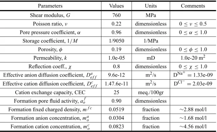
TABLE III
Modeling parameters for inclined wellbore.
Parameters Values Units Comments
Shear modulus,G 760 MPa
Poisson ratio,ν 0.22 dimensionless 0≤ν≤0.5 Pore pressure coefficient,α 0.96 dimensionless 0≤α≤1.0
Storage coefficient, 1/M 1/9050 1/MPa
Porosity,φ 0.19 dimensionless 0≤φ≤1.0 Permeability,k 1.0e-05 mD 1.0e-20 m2 Reflection coeff.,χ 0.8 dimensionless 0≤χ ≤1.0 Effective anion diffusion coefficient,De f fa 9.6e-12 m2/s DNa+=1.33e-09 Effective cation diffusion coefficient,Dce f f 1.47.6e-11 m2/s DCl−=2.03e-09
Cation exchange capacity, CEC 25 meq./100gr Formation pore fluid activity,aof 0.90 dimensionless
Formation fixed charged density,mf c 0.0519 fraction ∼2.88 mol/l Formation anion concentration,mao 0.0304 fraction ∼1.68 mol/l Formation cation concentration,mco 0.0823 fraction ∼4.56 mol/l
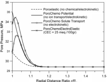
Figure 3 shows the pore pressure profile at time t = 0.01 day (∼15 minutes) into drilling for the case of high mud activity (amudf = 0.93 > aof = 0.90) using the complete solutions in Eq. 129 by combining the Laplace transform time inversion of Eqs. 88 and 103. Compared with the poroelastic and porochemoelastic response, it is obvious that there is a pressure increase at the wellbore wall due to the electrokinetic equilibrium requirement. This pressure discontinuity is not generated due to the chemical activity/salinity gradient between the mud and the formation as shown in the lumped chemical potential model (ignoring ion transport), but is a consequence of the electrostatic restriction of the negative fixed charge present on the shale pore surface. The chemical osmotic effect is to increase the near wellbore response of pore pressure in the shale formation. This makes sense since high mud activity induces additional osmotic flow into the formation. Figure 4 shows time evolution of the pore pressure profile for the porochemoelectroelastic solution along with the porochemoelastic solution in dashed lines. As time elapses, the initial osmotic pore pressure peak inside the formation decreases due to subsequent diffusion of solvent and ions. However, the fixed-charge induced pore pressure jump at the mud/shale interface stays constant through the course of time.
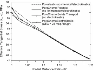
Figures 5 and 6 show, respectively, the corresponding effective radial and tangential stresses at
Fig. 3 – Pressure distribution in the formation aftert = 15 minutes into drilling for high mud activity (low mud salinity):
amudf =0.93>aof =0.90.
Fig. 4 – Pressure distribution in the formation at various time intervals into drilling for high mud activity (low mud salinity):
amudf =0.93>aof =0.90.
Fig. 6 – Effective tangential stress distribution in the formation aftert=15 minutes into drilling for high mud activity (low mud salinity):amudf =0.93>aof =0.90.
Fig. 7 – Effective radial stress distribution in the formation at various time intervals into drilling for high mud activity (low mud salinity):amudf =0.93>aof =0.90 and ignoring electrokinetic effect.
which promotes tensile fracturing failure in the formation. Unlike the porochemoelastic response, the ten-sile region for porochemoelectroelastic model does not vanish as time evolves, but enlarges as illustrated in Figures 7 and 8.
Fig. 8 – Effective radial stress distribution in the formation at various time intervals into drilling for high mud activity (low mud salinity):amudf =0.93>aof =0.90 with electrokinetic effect.
Fig. 9 – Pore pressure distribution in the formation aftert =15 minutes into drilling for low mud activity (high mud salinity):
amudf =0.87<aof =0.90.
Fig. 11 – Effective tangential stress distribution in the formation aftert=15 minutes into drilling for low mud activity (high mud salinity):amudf =0.87<aof =0.90.
Fig. 12 – Pore pressure distribution in the formation aftert=15 minutes at different CEC values for high mud activity (low mud salinity):amudf =0.93>aof =0.90.
It should be noted that the lumped chemical potential model (ignoring ion transport) does not provide bounds on the responses of the stress and pore pressure since it does not account for the electrokinetic restriction. Depending on the relative magnitudes of the chemical osmotic and electrokinetic effect, the contribution of one effect to the overall response can overshadow the other one. In the porochemoelec-troelastic model, the electrokinetic effects are manifested as a pressure discontinuity at the mud/shale boundary. This pressure difference is a direct function of the shale cation exchange capacity (CEC). Fig-ures 12 and 13 illustrate the effects of CEC on the pressure redistribution in the formation for high and low mud activity, respectively. It is observed that the higher the shale CEC, the higher the pressure increases at the mud/shale boundary. When the CEC is large enough, the resulting electrically induced pore pressure will eclipse the chemical osmotic effect.
CONCLUSIONS
A general isotropic porochemoelectroelastic formulation has been presented to account for electro-chemical effect in the overall response of chemically active porous media. Based on this formulation, a set of field and diffusion equations was developed to solve for the stress and pore pressure distribution. The corresponding analytical solution for the inclined wellbore problem in chemically active formations subjected to the three-dimensionalin-situstate of stress has been derived and presented in this paper.
From the present solutions, it is observed that the rate of diffusion is affected not only by the hy-draulic Darcy’s permeability, Fick’s solute diffusion coefficient, and the membrane reflection coefficient, but with the electrokinetic contribution that manifests itself as a boundary effect at the borehole wall. Proper modeling of the electrokinetic contribution requires the use of the commonly measured shale pa-rameters – Cation Exchange Capacity.
Via the inclined wellbore solution, effective stress and pore pressure analyses were carried out to study the electrokinetic and chemical effects on the overall poromechanic responses of the chemically active formations. Effective stress calculations show that the porochemoelectroelastic solution predictions differ substantially from the normal porochemoelastic and poroelastic approaches. Since wellbore stability analyses are usually performed based on effective stresses, ignoring the electrokinetic effects will mislead the predictions and assessment of potential problems in the field.
ACKNOWLEDGMENTS
Partial funds for this work were provided by the PoroMechanics Institute at the University of Oklahoma through the Rock Mechanics Consortium industry members.
RESUMO
ativa e ionizada tal como um folhelho submetido a um estado tridimensional de tensão. A solução analítica para esta geometria incorpora o acoplamento entre a deformação do sólido e o fluxo simultâneo de fluido e íons induzido pelos gradientes de poro pressão, potencial químico e potencial elétrico sob condições isotérmicas. O fluido residente na formação é modelado como uma solução eletrolítica composta de um solvente e cátions e anions dissolvidos. A abordagem analítica integra na solução o uso quantitativo da capacidade de troca catiônica (CTC) comumente obtida por medidas experimentais em amostras de folhelhos. Os resultados obtidos para as distribuições de tensões e poro pressão devido ao acoplamento eletroquímico são ilustrados e plotados na vizinhança do poço inclinado e comparados com as soluções clássicas poroelásticas com acoplamento químico.
Palavras-chave: perfuração, eletrocinética, poço inclinado, osmose, poromecânica, estabilidade.
REFERENCES
BIOTMA. 1941. General theory of three dimensional consolidation. J Appl Physics 12(2): 155–164.
CARTER JP AND BOOKER JR. 1982. Elastic consolidation around a deep circular tunnel. Int J Solids Struct 18(12): 1059–1074.
CHENGAH-D, SIDAURUKPANDABOUSLEIMANY. 1994. Approximate inversion of Laplace transform. Mathe-matica Journal 4(2): 76–82.
CORAPCIOGLUYM. 1991. Formulation of electro-chemico-osmotic process in soils. Transp Porous Media 6: 435–444.
COUSSYO. 2004. Poromechanics, Chichester: J Wiley & Sons, England, 298 p.
CUIL, CHENGAH-DANDABOUSLEIMANY. 1997. Poroelastic solution of an inclined borehole. ASME J Appl Mech 64: 32–38.
EHLERSWANDMARKERTB. 2001. A linear viscoelastic biphasic model for soft tissues based on the Theory of Porous Media. ASEM J BioMech Engrg 123: 418–424.
EKBOTE S AND ABOUSLEIMANY. 2006. Porochemoelastic solution for an inclined borehole in a transversely isotropic formation. J Engng Mech 132(7): 754–763.
ESRIG MI. 1968. Pore pressure, consolidation, and electrokinetics. J Soil Mech Found Div, Proceedings ASME 94(SM4): 899–921.
FARLOWSJ. 1993. Partial differential equations for scientists and engineers. New York, Dover Publications Inc., USA, p. 223–231.
GREGORHPANDGREGORCD. 1978. Synthetic membrane technology. Sci Amer 239: 112–128.
GRIMRE. 1968. Clay Mineralogy. New York, McGraw-Hill Book Co 2nded.
GUWY, LAIWMANDMOWVC. 1999. Transport of multi-electrolytes in charged hydrated biological soft tissues. Transp Porous Media 34(1-2): 143–157.
HANSHAWBB. 1964. Clays and Clay minerals. In: BRADLEYWF (Ed), National Conference. Proceedings of the 12thNational Conference, Atlanta Georgia, 1963, Pergamon Press, New York, USA, p. 397–421.