___________________________
1 Tecnólogo em Processamento de Dados, Prof. Adjunto da Universidade Tecnológica Federal do Paraná - Medianeira, Grupo de Pesquisa GROSAP. Medianeira, PR, E-mail:clbazzi@gmail.com.
2 Engº Mecânico, Prof. Associado da UNIOESTE/CASCAVEL/CCET/PGEAGRI/SBA, Grupos de Pesquisa GROSAP e GGEA, Pesquisador de Produtividade do CNPq. Cascavel, PR. E-mail: eduardo.souza@unioeste.br.
3Estatístico, Prof. Associado da UNIOESTE/CASCAVEL/CCET/PGEAGRI/SBA, Grupos de Pesquisa GROSAP e GGEA, Pesquisador de Produtividade do CNPq. PR. E-mail: miguel.opazo@unioeste.br.
4 Engª Agronoma, Profª. Associada da UNIOESTE/CASCAVEL/CCET/PGEAGRI/SBA, Grupos de Pesquisa GROSAP e GGEA, Pesquisador de Produtividade do CNPq. Cascavel, PR. E-mail: lucia.nobrega@unioeste.br.
5 Tecnólogo em Desenvolvimento de Sistemas de Informação, Pós-Graduando da UNIOESTE/CASCAVEL/CCET/PGEAGRI/SBA, Grupo de Pesquisa GROSAP, Bolsista da CAPES. Cascavel, PR, E-mail:davimarcondesrocha@gmail.com.
MANAGEMENT ZONES DEFINITION USING SOIL CHEMICAL AND PHYSICAL ATTRIBUTES IN A SOYBEAN AREA
CLAUDIO L. BAZZI1, EDUARDO G. SOUZA2, MIGUEL A. URIBE-OPAZO3, LÚCIA H. P. NÓBREGA4, DAVI M. ROCHA5
ABSTRACT: Several equipments and methodologies have been developed to make available precision agriculture, especially considering the high cost of its implantation and sampling. An interesting possibility is to define management zones aim at dividing producing areas in smaller management zones that could be treated differently, serving as a source of recommendation and analysis. Thus, this trial used physical and chemical properties of soil and yield aiming at the generation of management zones in order to identify whether they can be used as recommendation and analysis. Management zones were generated by the Fuzzy C-Means algorithm and their evaluation was performed by calculating the reduction of variance and performing means tests. The division of the area into two management zones was considered appropriate for the present distinct averages of most soil properties and yield. The used methodology allowed the generation of management zones that can serve as source of recommendation and soil analysis; despite the relative efficiency has shown a reduced variance for all attributes in divisions in the three sub-regions, the ANOVA did not show significative differences among the management zones.
KEYWORDS: Precision agriculture, spatial variability, fuzzy clustering, management zones, autocorrelation, cross-correlation.
DEFINIÇÃO DE UNIDADES DE MANEJO USANDO ATRIBUTOS QUÍMICOS E FÍSICOS DO SOLO EM UMA ÁREA DE SOJA
RESUMO: Diversos equipamentos e metodologias vêm sendo desenvolvidos para tornar a agricultura de precisão disponível, especialmente considerando o alto custo de sua implantação e de amostragem. Uma possibilidade interessante é definir a área em unidades menores de produção que podem ser tratadas de maneira diferente, servindo como fonte de recomendação e análise. Assim, o presente estudo utilizou propriedades físicas e químicas do solo e de produtividade visando à geração de unidades de manejo, a fim de identificar se estas podem ser usadas como recomendação e análise. Unidades de manejo foram geradas pelo algoritmo Fuzzy C-Means, e sua avaliação foi realizada por meio da redução da variância e realização de testes de comparação de médias. A divisão da área em duas unidades de manejo foi considerada adequada, e as médias apresentaram-se distintas da maioria das propriedades do solo e produtividade; a metodologia utilizada permitiu a geração de unidades de manejo que podem servir como fonte de recomendação e análise do solo. Apesar de a eficiência relativa demonstrar que houve redução da variância para todos os atributos na divisão em três sub-regiões, a ANOVA não apresentou diferenças significativas entre as unidades de manejo.
INTRODUCTION
The continued growth of precision agriculture technology (PA) promoted the emergence of machines equipped with sensors and equipment aiming at reducing costs and improving performance of production processes as well as allowing more detailed analysis of both soil and plants (chlorophyll meter, penetrometer, electrical conductivity meter, yield monitors, meters of vegetation index, among others).
According to KHOSLA et al. (2008), who conducts a research related to PA viability, there are some unknowns from producers that ultimately hinder its use in a more expressive way. Among the questions asked by the researcher, there are included some as: 1) Is it possible to determine the spatial variability of attributes in a less costly way? 2) Is the PA economically feasible? These questions are the focus of much research worldwide, aiming not only at answering them, but developing techniques and procedures that make affirmative answers to these questions. Thus, new forms of research on how to apply this technology study on lower sampling costs associated with sample size and the definition of management zones (TAYLOR et al., 2007; ROUDIER et al., 2008; RODRIGUES JR. et al., 2011; SUSZEK et al., 2012) emerges for making practical and economic PA.
A research to define management zones aims at dividing producing areas in smaller management zones should be treated differently, serving as a source of recommendation and analysis. Yield data, physical and chemical data of soil, electrical conductivity, topography and combination of them are routinely used to define these sub-regions, in addition to the use of statistical modeling of such attributes (RODRIGUES JR. et al., 2011).
For PEDROSO et al. (2010), there are several techniques to define management zones proposed in literature, and XIANG et al. (2007) make a division among techniques, considering two approaches: 1) Using empirical methods, which use frequency distribution of yield to divide the plot, usually in three or four management zones (SUSZEK, et al., 2012); 2) By means of cluster analysis methods such as K-means and Fuzzy C-means.
Quite feasible and obtaining satisfactory results (SUSZEK, et al., 2012), empirical techniques (normalized and standatized yield) make use of crop yield data for definition of management zones and assume that this figure corresponds to crop response, i.e., it does not aim at identifying those attributes affecting the yield, this is a later stage of the process. They also consider that techniques become more accurate the larger it is the number of used crops.
Clustering methods are highly suggested for defining management zones (YAN et al., 2007; ILIADIS et al., 2010) and include the use of several attributes such as electrical conductivity, slope and soil texture, nitrogen, among others and simultaneous use of these attributes. Although there is a possibility of any attribute can be related to crop yield, for DOERGE (2000), the ideal one is using predictable spatial information sources correlated with yield.
The most commonly used clustering methods to define management zones correspond to the K-means algorithm (RODRIGUES JR. et al., 2011; ORTEGA & SANTIBÁÑEZ, 2007) and Fuzzy C-Means (YAN et al., 2007). Both are differentiated by the robustness and are also set up according to Fuzzy C-Means method, which incorporated the theory of Fuzzy logic to the division algorithm.
MATERIAL AND METHODS
The study was carried out in a 19.8 ha commercial farming area, in Serranópolis do Iguaçu/PR, under the following geographical coordinates: 25º26'49''S and 54º04'59''W and 280 m average altitude (Figure 1). The area delimitation and sampling points’ sites were obtained with a GPS receiver Trimble Geo Explorer XT 2005 and PathFinder software.
a) Area location in Brazil b) View of the area with the sampling grid FIGURE 1. Visualization of the experimental area and experimental grid.
Fifty eight sampling points were defined (2.93 points ha-1, roughly equivalent to the 2.2 points ha-1 suggested by FRANZEN & PECK, 1995) using an irregular grid (Figure 1), 30 m minimum distance and 497 m maximum distance, where data were collected on soybean yield, soil chemical parameters (C, pH, H+ Al, Ca, Mg, K, Cu, Zn, Fe, Mn) and textural (silt, sand, clay) properties, in addition to water content and soil penetration resistance at the layers 0 to 0.1 m (SPR010), 0.1-0.2 m (SPR1020), 0.2-0.3 m (SPR2030) depth and average soil compaction at 0 to 0.3m (SPRAVG030) depth. The irregular grid was created considering the planting line.
Each sample point was represented by the total mass collected on two lines in a path of one meter and, as the spacing was 0.45 m, each sample point was represented by an area of approximately 0.9 m2 (TAVARES-SILVA et al., 2012). The harvested product was referred to the threshing process and water content determination; subsequently yield values were corrected for 13% water content. Soil samples were collected with a hoe and shovel. They were packed in bags and sent for chemical analysis.
Four measurements of soil penetration resistance were performed from 0 to 0.30 m layer at each sampling point, by a Falker PGL 1020 electronic meter of soil penetration resistance.
Data were statistically analyzed by means of exploratory analysis, by calculating the mean, median, minimum, maximum, standard deviation and coefficient of variation (CV). The CV was considered low (homoscedasticity) when CV ≤ 10%, medium when 10% < CV ≤ 20%, high when 20% < CV ≤ 30% and very high (heteroscedasticity) when CV > 30% (PIMENTEL & GARCIA, 2002). In order to evaluate the data normality at 5% probability, Anderson-Darling and Kolmogorov-Smirnov tests were performed, and those with normality for at least one of the tests were considered normal.
Usually, the definition of management unit aims at serving as a source of recommendation and analysis for several years (DOERGE, 2000). Therefore, stable and predictable sources of spatial information should be used, which are also correlated with yield. Non-stable sources of information can also be used to define management zones and adjust the amount of nutrients in a certain year. Thus, two approaches were used to generate management units: 1) statistics, where all the studied
attributes (not all that are considered stable) are used; and 2) agronomic, taking into account only the attributes of soil resistance to penetration and texture ones, considered as stable.
Aiming at evaluating the spatial correlation between the attributes and yield, the cross-correlation was used (BONHAM et al., 1995, Equation 1). It make possible to verify which attributes influenced positively or negatively on soybean yield, and if a sample is spatially autocorrelated. 2 2 1 1
*
*
*
Z Y n i n j j i ij YZm
m
W
Z
Y
W
I
where IYZ- Degree of spatial association between Y and Z variables, ranging from -1 to 1, as it is followed: positive correlation IYZ 0 and negative correlation IYZ0, - Wij correspond to the ij
element of spatial association matrix, calculated by Wij(1/(1Dij)), so that, D is the distance ij between i and j points; Yi- transformed Y value at point i. The transformation is to have a zero
average, by the formula:Yi (YiY) , where Y is the sample average of Y, Z variables - j
transformed Z variable at j point. Transformation occurs to have a zero average by the formula:
) Z (Z
Zj j , where Zthe sample average of variable Z. W – corresponds to the sum of spatial association degrees obtained by the matrix W , for ij i j.
2 Y
m - Sample variance of the Y variable. 2
Z
m - corresponds to the sample variance of Z variable.
After the IYZ calculation, the spatial correlation matrix was generated, which also presents the
significance of the test in addition to the calculated index IYZ, considering data permutation, where
several correlation tests are performed by permuting values of one of the variables to be compared. It remains the points’ sites and the values of a position are randomly replaced by one from another point. This technique requires a high computational degree. Under the hypothesis H0, Yi random
variables are independent and identically distributed and thus, all the permutations of Yi values among areas are equally likely. Therefore, the p value of the test is given by Equation 2.
1 n n 1,..., j , I ) ContIf(I valor p (1) (j)
where n is the number of permutations (default is 999 permutations) I - corresponds to the index
calculated by the equation (1).
The null hypothesis is rejected with significance α if p-value < α, i.e., H0 is rejected with 0.05
of significance if p-value < 0.05.
For both studied situations (statistical and agronomic), matrices of spatial correlation were generated. In order to select the layers that will serve as input data for the Fuzzy C-Means algorithm, the following procedure was used:
1. Elimination of layers with spatial dependence and not significant at 95% significance; 2. From layers with spatial dependence, those with no correlation with soybean yield were removed.
3. The descending order was calculated, considering the degree of correlation with yield; 4. The redundant layers were eliminated (those which correlated with each other), preferring those with lower correlation with yield.
(1)
In order to draw the thematic maps, the sample data were interpolated and selected in the analysis of spatial correlation as self-correlated and influence on soybean yield. The surface was represented by 5 x 5 m polygons, representing 25 m2. It was used the interpolation method of inverse distance, with an interpolation window of 10 neighbors.
The generation of management zones was performed by Fuzzy C-Means clustering technique (BEZDEK, 1981), which considers a data set X {x1,..,xn} where xk corresponds to a feature
vector P
kp k
k x x R
x { 1,.., } for all k{1,..n}, and R is the p-dimensional space. It is aimed at P
finding a fuzzy pseudo partition which corresponds to a family of fuzzy sets of X c, which
represents the data structure as best as possible and is denoted by P{A1,A2,...AC}, satisfying
c 1 i k i(x ) 1A and
n 1 k k i(x ) n
A
0 where K{1,2,..,n} and n represents the number of elements
(lines) matrix X.
The algorithm is guided with parameters on the number of desired clusters (C), a distance measure that defines the allowable distance among points and centroids (m(1,)) and error was
used as a stopping criterion (
104). The position of each centroid is calculated considering the distance passed initially by the parameter (preferably to be m = 1.3). For each C, c(t)(t) 1 ,..,v
v is
calculated by (Equation 3) for P partition, being (t) t{1,..,n}the iteration. The vector
i
v corresponds to the clustering center and Ai is the data weighted average. The weight of xk is the m-th power of its pertinence degree to the Ai fuzzy set.
n k m k i n k k m k i i X A x x A v 1 1 )] ( [ )] ( [Calculation of the pertinence degree of xk to the class Ai (Equation 4) is performed for each X
xk and for all i{1,..,c}, if ||x v(t)||2 0
i
k .
1 1 m 1 c 1
j k j(t) 2
2 (t) i k k 1) (t i || v x || || v x || ) (x A
where ||xk vi(t)||2 represents the distance between xk and vi.
As stopping criterion, P and (t) P(t1) are compared, and if |P(t)P(t1)|ε
, the algorithm is terminated and the classification is performed by considering the pertinence generated in the last iteration.
Since we worked on several data layers, data were normalized (Equation 5) (MIELKE & BERRY, 2007), whereas there can have different attributes measured and that influence on the clustering process. Range Median P P i iNorm
where PiNorm is the normalized pixel value; Pi is the pixel value i to be normalized.
(4)
Eight thematic maps were generated, classified according to the division in management zones, considering respectively 2, 3, 4 and 5 sub-regions in the plot.
In order to carry out an evaluation, management zones were used for physical and chemical data and yield of soybean aiming at identifying if the generated zones are significantly different for each attribute. Two parameters were used in this evaluation:
1. Relative Efficiency (RE): evaluates whether there was reduction of total variance of the attribute evaluated with the division into management zones (Equation 6); it was considered an adequate clustering when RE > 1 so, the more efficient the higher RE;
2 MZ 2 AREA
S S
RE (6)
where S2MZ is the sum of the variance in yield of each management unit, calculated separately, considering the proportion of the total area representing the management zone; 2
AREA
S - variance of yield related to the area.
2. Variance analysis: evaluates whether the management zones are associated with statistically different attributes, assuming that data have normal distribution and are internally independent in each sub-region.
RESULTS AND DISCUSSION
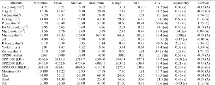
The attributes P, K and Zn were classified as heteroscedastic (CV > 30%) and Fe, soil penetration resistance 0 to 10 cm (SPR_0_10), and sand as high CV. For other attributes, only pH could be classified as homoscedastic.
Ca, C, Cu, H+Al, Mg, Mn, yield, soil penetration resistance from 10 to 20 cm (SPR1020), from 20 to 30 cm (SPR2030), and average soil penetration resistance (SPRAVG030) (MPa), moisture, silt, and clay were classified with moderate CV. Cu, P, K and Zn presented some positive asymmetry, silt negative asymmetry and other attributes, symmetrical distribution. Only C and average SPR showed kurtosis classified as platikurtic, and Cu, P, K and Zn were classified as leptokurtic (Table 1). Only P attribute did not show normal distribution.
TABLE 1. Data descriptive statistics.
Attribute Minimum Mean Median Maximum Range SD C V Asymmetry Kurtosis
Ca (cmolc dm-3) 4.71 6.21 6.19 8.02 3.31 0.70 11.2 (m) 0.02 (a) -0.13 (A)
C (g dm-3) 13.36 16.67 16.70 20.78 7.42 1.86 11.2 (m) 0.17 (a) -0.93 (B)
Cu (mg dm-3) 7.20 9.37 9.30 16.50 9.30 1.51 16.1(m) 1.96 (b) 7.74 (C)
Fe (mg dm-3) 14.00 25.33 25.00 43.00 29.00 6.12 24.1(h) 0.60 (a) 0.14 (A)
P (mg dm-3)* 6.70 20.48 17.70 57.30 50.60 10.41 50.8(vh) 1.18 (b) 1.75 (C)
H+Al (cmolc dm-3) 2.95 3.65 3.69 4.96 2.01 0.52 14.1(m) 0.55 (a) -0.07 (A)
Mg (cmolc dm-3) 1.56 2.76 2.69 3.99 2.43 0.49 17.8 (m) 0.41(a) 0.09 (A)
Mn (mg dm-3) 83.00 117.33 116.00 167.00 84.00 20.38 17.4 (m) 0.28(a) -0.67 (A)
pH 4.90 5.65 5.70 6.20 1.30 0.29 5.1(l) -0.17 (a) -0.01(A)
K (cmolc dm-3) 0.18 0.38 0.35 1.14 0.96 0.18 46.3(vh) 2.32 (b) 6.34 (C)
Yield (t ha-1) 2.91 4.47 4.52 6.36 3.44 0.64 14.4 (m) 0.32 (a) 1.30 (A)
Zn (mg dm-3) 3.10 5.59 5.20 11.70 8.60 1.91 34.2 (vh) 1.32 (b) 1.71 (C)
SPR010 (kPa) 2261 3988 3879 4560 3910 923 23.1 (h) 0.58 (a) -0.09 (A)
SPR1020 (kPa) 3566.6 5115.3 5217.7 6509.0 2942.4 727.1 14.2 (m) -0.08 (a) -0.63 (A)
SPR2030 (kPa) 3451.9 4752.6 4757.6 6089.1 2637.2 636.4 13.4 (m) 0.21 (a) -0.45 (A)
SPRAVG030(kPa) 3841.0 4874.1 4894.5 6115.0 2273.9 538.8 11.0 (m) 0.20 (a) -0.80 (B)
Moisture (%) 10.180 13.22 12.93 17.58 7.40 1.81 13.7 (m) 0.39 (a) -0.40 (A)
Clay 44.00 53.12 53.50 68.00 24.00 5.56 10.5 (m) 0.46 (a) -0.34 (A)
Sand 9.00 14,38 14.00 23.00 14.00 3.09 21.5 (h) 0.47 (a) -0.29 (A)
Silt 20.00 32.50 33.00 41.00 21.00 4.43 13.6 (m) -0.93 (c) 1.13 (A)
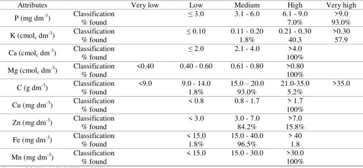
Considering the classification proposed by COSTA & OLIVEIRA (2001) for soil chemistry, the attributes Ca, Cu, Mg and Mn presented high availability throughout the area (Table 2). C and Fe presented low availability at a sampling point, but in most sampling points (93% and 96.5%, respectively) could be classified as medium level of availability. Zn also presented with medium level in 84.2% of samples.
TABLE 2. Levels of interpretation of soil chemical properties with the percentage of the studied sampling points.
Attributes Very low Low Medium High Very high P (mg dm-3) Classification ≤ 3.0 3.1 - 6.0 6.1 - 9.0 >9.0
% found 7.0% 93.0% K (cmolc dm-3) Classification % found ≤ 0.10 0.11 - 0.20 1.8% 0.21 - 0.30 40.3 >0.30 57.9
Ca (cmolc dm-3) Classification % found ≤ 2.0 2.1 - 4.0 100% >4.0
Mg (cmolc dm-3) Classification % found <0.40 0.40 - 0.60 0.61 - 0.80 >0.80 100%
C (g dm-3) Classification <9.0 9.0 - 14.0 15.0 – 20.0 21.0-35.0 >35.0
% found 1.8% 93.0% 5.2% Cu (mg dm-3) Classification < 0.8 0.8 - 1.7 > 1.7
% found 100% Zn (mg dm-3) Classification < 3.0 3.0 - 7.0 >7.0
% found 84.2% 15.8% Fe (mg dm-3) Classification % found < 15.0 1.8% 15.0 - 40.0 96.5% > 40 1.8
Mn (mg dm-3) Classification < 15.0 15.0 - 30.0 >30.0
% found 100%
Source: COSTA & OLIVEIRA (2001)
Selected Layers Statistic approach:
Using the spatial correlation matrix, Mg layer was selected to generate management zones, considering that:
1. Withdrew layers: Ca, C, Fe, P, H_AL, Mn, SPR010, pH, K, due to non-significance of the spatial dependence. (Result matrix Figure 2);
2. Withdrew layers: average SPR, SPR1020, SPR2030, and silt, due to lack of correlation of them with soybean yield;
3. After ordering the remaining layers (Cu, Mg, moisture, Zn, clay, sand) in ascending order by degree of correlation with yield, redundant layers were eliminated.
YIELD 0.0038
CU -0.0682 0.0877
MG 0.0830 -0.1488 0.1747
MOISTURE -0.0364 0.1126 -0.1320 0.1204
ZN 0.0454 -0.0847 0.1073 -0.0749 0.0337
AVG_RMP -0.0015 -0.0064 0.0004 -0.0138 0.0005 -0.0468
SPR1020 -0.0177 0.0367 -0.0480 0.0432 -0.0252 -0.0427 -0.0282
SPR2030 0.0134 -0.0221 0.0215 -0.0337 0.0014 -0.0392 -0.0352 -0.0354
CLAY 0.0484 -0.0996 0.1337 -0.1254 0.0668 0.0009 -0.0365 0.0238 0.0826
SILT -0.0102 0.0243 -0.0320 0.0407 -0.0207 -0.0027 0.0146 -0.0061 0.0066 -0.0293
SAND -0.0718 0.1431 -0.1930 0.1658 -0.0897 0.0021 0.0444 -0.0338 -0.1567 0.0330 0.2326
YIELD CU MG MOIST ZN SPRAVG030 SPR1020 SPR2030 CLAY SILT SAND
Agronomic approach:
Using the spatial correlation matrix (Figure 3), sand layer was selected for generation of management zones, considering that:
1. Withdrew layers: SPR010, due to non-significance of the spatial dependence;
2. Withdrew layers: SPRAVG030, SPR1020, SPR2030, and silt, due to their lack of correlation with soybean yield;
3. After ordering the remaining layers (clay and sand) in ascending order by degree of correlation with yield, redundant layers were eliminated.
YIELD 0.0038
AVG_SPR -0.0015 -0.0468
SPR010 -0.0106 -0.0291 -0.0091
SPR1020 -0.0177 -0.0427 -0.0251 -0.0282
SPR2030 0.0134 -0.0392 -0.0311 -0.0352 -0.0354
CLAY 0.0484 0.0009 -0.0212 -0.0365 0.0238 0.0826
SILT -0.0102 -0.0027 0.0057 0.0146 -0.0061 0.0066 -0.0293
SAND -0.0718 0.0021 0.0298 0.0444 -0.0338 -0.1567 0.0330 0.2326
YIELD SPRAVG030 SPR010 SPR1020 SPR2030 CLAY SILT SAND
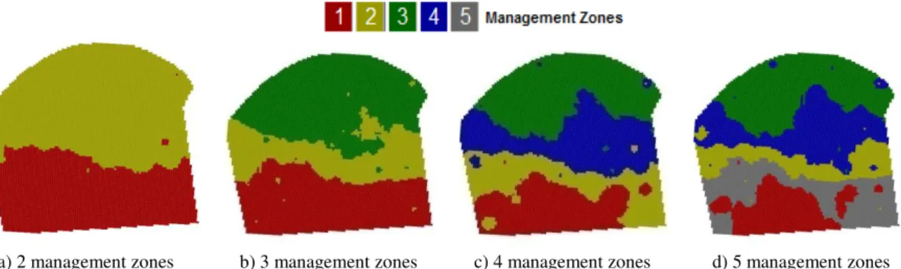
Four thematic maps were generated for each approach, for divisions in 2, 3, 4 and 5 management zones, respectively (Figures 4 and 5) using the Fuzzy C-Means algorithm with parameters m = 1.3 and stopping criterion or error = 0.0001.
a) 2 management zones b) 3 management zones c) 4 management zones d) 5 management zones
FIGURE 4. Division of the area into management zones using Fuzzy logic and Mg layer, selected by means of cross spatial correlation matrix to statistic approach.
a) 2 management zones b) 3 management zones c) 4 management zones d) 5 management zones
FIGURE 5. Division of the area into management zones using Fuzzy logic and sand layer, selected by means of cross spatial correlation matrix to agronomic approach.
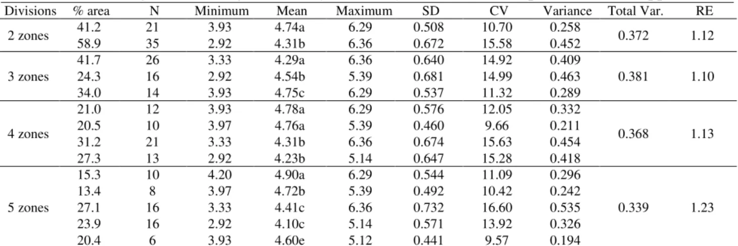
analysis of variance, only the divisions in 2 and 3 sub-regions were considered different on average, indicating that each class has different productive potential. Thus, divisions in 2 and 3 zones in statistic approach were considered significant and maintained to evaluate whether they can serve as source of recommendation and analysis of other attributes.
The agronomic approach did not show good results for the studied divisions as RE < 1, while ANOVA showed that the data sets had equal averages for almost all cases.
TABLE 3. Descriptive statistics and relative efficiency of yield data (t ha-1) separated by management zone generated by the Fuzzy C-Means technique for statistic approach.
Divisions % area N Minimum Mean Maximum SD CV Variance Total Var. RE
2 zones 41.2 58.9 21 35 3.93 2.92 4.31b 4.74a 6.36 6.29 0.508 0.672 10.70 15.58 0.452 0.258 0.372 1.12
3 zones
41.7 26 3.33 4.29a 6.36 0.640 14.92 0.409
0.381 1.10
24.3 16 2.92 4.54b 5.39 0.681 14.99 0.463
34.0 14 3.93 4.75c 6.29 0.537 11.32 0.289
4 zones
21.0 12 3.93 4.78a 6.29 0.576 12.05 0.332
0.368 1.13
20.5 10 3.97 4.76a 5.39 0.460 9.66 0.211
31.2 21 3.33 4.31b 6.36 0.674 15.63 0.454
27.3 13 2.92 4.23b 5.14 0.647 15.28 0.418
5 zones
15.3 10 4.20 4.90a 6.29 0.544 11.09 0.296
0.339 1.23
13.4 8 3.97 4.72b 5.39 0.492 10.42 0.242
27.1 16 3.33 4.41c 6.36 0.732 16.60 0.535
23.9 16 2.92 4.10c 5.14 0.571 13.92 0.326
20.4 6 3.93 4.60e 5.12 0.441 9.57 0.194
SD – Standard deviation, CV - Coefficient of Variation, N - Number of sample elements; Total Var. - Total variance, obtained by the representation of each management unit and the variance found. Means followed by same letter do not differ among themselves by Tukey test at 5% probability of error.
TABLE 4. Descriptive statistics and relative efficiency of yield data (t ha-1) separated by management zone generated by the Fuzzy C-Means technique for agronomic approach.
Divisions % area N Minimum Mean Maximum SD CV Variance Total Var. RE
2 zones 67.3 32 2.92 4.52a 6.29 0.66 14.7 14.12 0.426 0.978
32.7 24 3.33 4.41a 6.36 0.63 14.3 9.52
3 zones
60.9 30 2.92 4.53a 6.29 0.69 15.1 14.08
0.447 0.935
18.4 10 3.33 4.54a 6.36 0.80 17.6 6.41
20.7 16 3.59 4.33ab 4.92 0.46 10.5 3.32
4 zones
56.8 27 2.92 4.53a 6.29 0.71 15.7 13.59
0.454 0.920
12.7 8 3.85 4.43b 4.81 0.38 0.09 1.12
15.0 12 3.59 4.34a 4.92 0.49 0.11 2.92
15.5 9 3.33 4.53a 6.36 0.86 0.19 6.58
5 zones
30.0 8 2.92 4.62a 6.29 1.05 22.9 8.89
0.576 0.725
12.0 7 3.85 4.59b 6.36 0.84 18.3 4.93
13.8 12 3.59 4.34c 4.92 0.49 11.4 2.92
14.4 8 3.33 4.30d 5.14 0.55 12.7 2.39
29.8 21 3.47 4.52ce 5.39 0.52 11.5 5.68
SD – Standard deviation, CV - Coefficient of Variation, N - Number of sample elements; Total Var. - Total variance, obtained by the representation of each management unit and the variance found. Means followed by same letter do not differ among themselves by Tukey test at 5% probability of error.
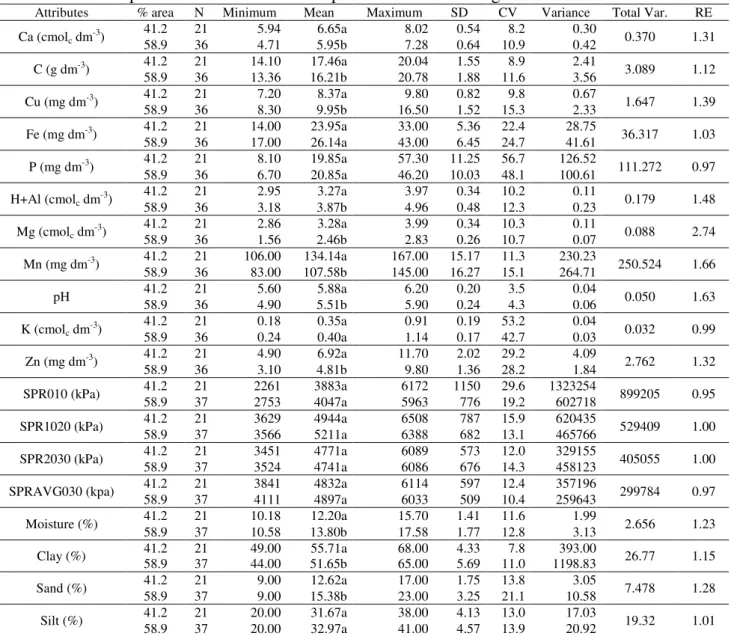
TABLE 5. Descriptive statistics of the data separated into two management zones.
Attributes % area N Minimum Mean Maximum SD CV Variance Total Var. RE
Ca (cmolc dm-3) 41.2 58.9 21 36 4.71 5.94 5.95b 6.65a 7.28 8.02 0.54 0.64 10.9 8.2 0.30 0.42 0.370 1.31
C (g dm-3) 41.2 21 14.10 17.46a 20.04 1.55 8.9 2.41 3.089 1.12
58.9 36 13.36 16.21b 20.78 1.88 11.6 3.56
Cu (mg dm-3) 41.2 21 7.20 8.37a 9.80 0.82 9.8 0.67 1.647 1.39
58.9 36 8.30 9.95b 16.50 1.52 15.3 2.33
Fe (mg dm-3) 41.2 21 14.00 23.95a 33.00 5.36 22.4 28.75 36.317 1.03
58.9 36 17.00 26.14a 43.00 6.45 24.7 41.61
P (mg dm-3) 41.2 21 8.10 19.85a 57.30 11.25 56.7 126.52 111.272 0.97
58.9 36 6.70 20.85a 46.20 10.03 48.1 100.61
H+Al (cmolc dm-3) 41.2 58.9 21 36 3.18 2.95 3.87b 3.27a 4.96 3.97 0.34 0.48 12.3 10.2 0.11 0.23 0.179 1.48 Mg (cmolc dm-3) 41.2 58.9 21 36 1.56 2.86 2.46b 3.28a 2.83 3.99 0.34 0.26 10.7 10.3 0.11 0.07 0.088 2.74
Mn (mg dm-3) 41.2 21 106.00 134.14a 167.00 15.17 11.3 230.23 250.524 1.66
58.9 36 83.00 107.58b 145.00 16.27 15.1 264.71
pH 41.2 58.9 21 36 5.60 4.90 5.51b 5.88a 5.90 6.20 0.20 0.24 3.5 4.3 0.06 0.04 0.050 1.63 K (cmolc dm-3) 41.2 58.9 21 36 0.24 0.18 0.40a 0.35a 1.14 0.91 0.19 0.17 42.7 53.2 0.04 0.03 0.032 0.99
Zn (mg dm-3) 41.2 21 4.90 6.92a 11.70 2.02 29.2 4.09 2.762 1.32
58.9 36 3.10 4.81b 9.80 1.36 28.2 1.84
SPR010 (kPa) 41.2 58.9 21 37 2261 2753 3883a 4047a 6172 5963 1150 776 29.6 19.2 1323254 602718 899205 0.95
SPR1020 (kPa) 41.2 58.9 21 37 3629 3566 4944a 5211a 6388 6508 787 682 15.9 13.1 465766 620435 529409 1.00 SPR2030 (kPa) 41.2 58.9 21 37 3451 3524 4771a 4741a 6086 6089 573 676 12.0 14.3 458123 329155 405055 1.00
SPRAVG030 (kpa) 41.2 58.9 21 37 3841 4111 4832a 4897a 6033 6114 597 509 12.4 10.4 259643 357196 299784 0.97
Moisture (%) 41.2 58.9 21 37 10.18 10.58 13.80b 12.20a 17.58 15.70 1.41 1.77 11.6 12.8 3.13 1.99 2.656 1.23 Clay (%) 41.2 58.9 21 37 49.00 44.00 51.65b 55.71a 65.00 68.00 4.33 5.69 11.0 7.8 1198.83 393.00 26.77 1.15 Sand (%) 41.2 58.9 21 37 9.00 9.00 15.38b 12.62a 23.00 17.00 1.75 3.25 13.8 21.1 10.58 3.05 7.478 1.28 Silt (%) 41.2 58.9 21 37 20.00 20.00 31.67a 32.97a 41.00 38.00 4.13 4.57 13.0 13.9 20.92 17.03 19.32 1.01 SD – Standard deviation, CV - Coefficient of Variation, N - Number of sample elements; Total Var. - Total variance, Means followed by same letter do not differ among themselves by Tukey test at 5% probability of error; RE - Relative Efficiency; soil penetration resistance from 0 to 10 cm (SPR010), from 10 to 20 cm (SPR1020), from 20 to 30 cm (SPR2030), and average soil penetration resistance (SPRAVG030).
For other studied attributes, they were all different by analysis of variance and with R > 1, indicating that the division can be taken as a source of recommendation and analysis.
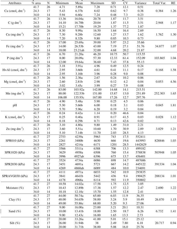
When three management zones were taken into account (Table 6), RE > 1 was verified for all the studied attributes, except for silt, i.e., division was satisfactory for all other attributes with reduced variance. Despite this fact, data sets were different only for the attributes Ca, Mg, Mn, pH and moisture, as well as for silt. Thus, it is concluded that the division into three management zones did not show good results for analysis and recommendation, since most of the attributes presented equality among management zones.
TABLE 6. Descriptive statistics of the data separated into three management zones.
Attributes % area N Minimum Mean Maximum SD CV Variance Total Var. RE
Ca (cmolc dm-3)
41.7 26 4.71 5.89a 7.28 0.71 12.1 0.51
0.384 1.26
24.3 17 5.43 6.37b 8.02 0.62 9.7 0.38
34.0 14 5.94 6.60c 7.24 0.48 7.3 0.23
C (g dm-3) 41.7 24.3 26 17 13.36 14.10 16.78b 16.04a 20.04 20.78 1.87 1.87 11.7 11.5 3.51 3.51 2.948 1.17
34.0 14 15.21 17.70b 19.29 1.37 77.2 1.87
Cu (mg dm-3) 41.7 24.3 26 17 8.30 7.30 9.28b 9.99a 12.60 16.50 1.27 1.64 16.4 13.7 2.69 1.62 1.762 1.30
34.0 14 7.20 8.32b 9.80 0.85 10.3 0.73
Fe (mg dm-3) 41.7 24.3 26 17 17.00 14.00 26.53b 25.69a 43.00 39.00 7.19 5.97 23.2 27.1 35.66 51.76 34.877 1.07
34.0 14 18.00 23.21ab 32.00 4.68 20.2 21.87
P (mg dm-3) 41.7 24.3 26 17 6.70 8.00 20.09a 21.20a 57.30 46.20 12.33 10.75 50.7 61.4 115.55 152.09 103.865 1.04
34.0 14 12.00 19.64a 36.60 7.43 37.8 55.13
H+Al (cmolc dm-3)
41.7 26 3.18 3.91a 4.96 0.49 12.5 0.24
0.168 1.58
24.3 17 2.95 3.66b 4.61 0.41 11.1 0.17
34.0 14 2.95 3.16b 3.96 0.28 9.0 0.08
Mg (cmolc dm-3)
41.7 26 1.56 2.36a 2.67 0.24 10.2 0.06
0.053 4.56
24.3 17 2.60 2.81b 2.98 0.12 4.2 0.04
34.0 14 3.02 3.45c 3.99 0.27 7.9 0.08
Mn (mg dm-3) 41.7 24.3 26 17 83.00 88.00 122.53b 103.92a 151.00 142.00 15.87 14.68 14.1 13.0 215.51 251.89 252.303 1.65
34.0 14 106.00 135.93c 167.00 17.26 12.7 297.76
pH
41.7 26 4.90 5.48a 5.90 0.25 4.5 0.06
0.045 1.81
24.3 17 5.30 5.66b 6.00 0.18 3.1 0.03
34.0 14 5.70 5.96c 6.20 0.19 3.2 0.04
K (cmolc dm-3)
41.7 26 0.24 0.42a 1.14 0.20 46.6 0.04
0.028 1.12
24.3 17 0.25 0.40a 0.91 0.17 41.5 0.03
34.0 14 0.18 0.29b 0.71 0.13 42.6 0.02
Zn (mg dm-3) 41.7 24.3 26 17 3.10 3.60 5.51a 4.80a 10.60 9.80 1.70 1.49 31.0 30.9 2.21 2.89 3.029 1.21
34.0 14 5.10 7.14b 11.70 2.03 28.5 4.13
SPR010 (kPa)
41.7 27 2753 4239a 5963 743 17.5 552411
828846 1.03
24.3 17 2261 3400b 4630 666 19.6 443993
34.0 14 2827 4214a 6171 1201 28.5 1442629
SPR1020 (kPa)
41.7 27 3566 5311a 6388 706 13.3 499182
503948 1.05
24.3 17 3629 4958a 6508 760 15.4 578838
34.0 14 3996 4927ab 6396 675 13.7 456401
SPR2030 (kPa)
41.7 27 3524 4734a 6086 698 14.7 487686
391334 1.04
24.3 17 3451 4691a 5721 667 14.2 445122
34.0 14 4269 4860ab 6089 484 10.0 234691
SPRAVG030 (kPa)
41.7 27 4111 4971a 6033 542 10.9 293835
288134 1.01
24.3 17 3841 4641b 5442 436 9.4 190425
34.0 14 4178 4968a 6114 592 11.9 350802
Moisture (%)
41.7 27 10.58 14.02a 17.58 1.75 12.5 3.05
2.690 1.22
24.3 17 10.43 12.89b 17.38 1.57 12.2 2.47
34.0 14 10.18 12.10c 15.70 1.55 12.8 2.41
Clay (%)
41.7 27 44.00 50.74a 65.00 6.03 11.9 36.35
26.870 1.15
24.3 17 48.00 54.65b 58.00 3.24 5.9 10.49
34.0 14 49.00 55.86c 68.00 5.20 9.3 27.06
Sand (%)
41.7 27 9.00 16.00a 23.00 3.21 20.1 10.31
6.732 1.41
24.3 17 10.00 13.41b 18.00 2.50 18.7 6.26
34.0 14 9.00 12.43c 16.00 1.65 13.3 2.73
Silt (%)
41.7 27 20.00 33.26a 41.00 5.01 15.1 25.12
20.717 0.94
24.3 17 26.00 31.94b 38 2.49 7.80 6.18
34.0 14 20.00 31.71b 38.00 5.08 16.0 25.76
SD – Standard deviation, CV - Coefficient of Variation, N - Number of sample elements; Total var. - Total variance. Means followed by same letter do not differ among themselves by Tukey test at 5% probability of error; RE - Relative Efficiency;
soil penetration resistance from 0 to 10 cm (SPR010), from 10 to 20 cm (SPR1020), from 20 to 30 cm (SPR2030), and average soil penetration resistance (SPRAVG030).
CONCLUSIONS
• The used methodology allowed the generation of management zones that can serve as source of recommendation and soil analysis;
• The subdivision into two management zones was considered the best by allowing zones with a greater number of different attributes among classes;
• The program “Software for Definition of Management Zones-SDUM” enabled a quick and easy creation of management zones, despite the complexity of the applied methodology;
• Despite the relative efficiency showing reduced variance for all attributes in divisions in the three sub-regions, ANOVA showed no consistent results.
• The agronomic approach did not show good results for the division of management units, so, it was not possible to identify different productive potential sites of the studied area.
ACKNOWLEDGEMENTS
The Araucária Foundation (Fundação Araucária), the Capes Foundation – Brazilian Ministry of Education, Technological Foundation Park Itaipu (for the doctorate scholarship); and the National Council for Scientific and Technological Development (CNPq).
REFERENCES
BEZDEK, C. J. Pattern recognition with fuzzy objective function algorithms. New York: Plenum
Press, 1981. 256 p.
BONHAM, C.D.; REICH, R.M; LEADER, K.K. Spatial cross-correlation of Bouteloua gracilis with site factors, Grassland Science, Tochigi, v.41, n.1, p.196-201, 1995.
COSTA, J.M.; OLIVEIRA, E.F. de. Fertilidade do solo e nutrição de plantas: culturas:
soja-milho-trigo-algodão-feijão. 2. ed. Campo Mourão: COAMO, COODETEC, 2001. 93 p.
DOERGE, T.A. Management zones concepts. Site-specific management guidelines. Norcross:
Potash & Phosphate Institute, 2000, 135 p.
Franzen, D.W., and T.R. Peck. Field soil sampling density for variable rate fertilization. Journal of Prodution Agriculture, Madison, v.8, n.4, p.568–574, 1995.
ILIADIS, L.S.; VANGELOUDH, M.; SPARTALIS,S. An inteligent system employing an enhanced fuzzy C-Means clustering model: Application in the case of forest fires. Computers and Eletronics in Agriculture, Netherlands, v.70, n.1, p.276-284, 2010.
KHOSLA, R.; INMANN, D.; WESTFALL, D.G.; REICH, R. M.; FRASIER, M.; MZUKU, M.; KOCH, B.; HORNUNG, A. A synthesis of multi-disciplinary research in precision agriculture: site-specific management zones in the semi-arid western Great Plains of the USA. Precision
Agriculture, Dordrecht, v.9, n.1, p. 85-100, 2008.
MIELKE, P.W.J; BERRY, K.J. Permutation methods: a distance function approach. New York: Springer, 2007. 439 p.
ORTEGA, R.A.; SANTIBÁÑEZ, O.A. Determination of management zones in corn (Zea mays L.)
based in soil fertility. Computers and Eletronics in Agriculture, Netherlands, v.58, n.1, p.49-59,
2007.
PIMENTEL, F.G.; GARCIA, G.H. Estatística aplicada a experimentos agronômicos e florestais.
Piracicaba: Biblioteca de Ciências Agrárias Luiz de Queiroz, 2002. 307 p.
RODRIGUES JUNIOR, F.A.; VIEIRA, L.B.; QUEIROZ, D.M.; SANTOS, N.T. Geração de zonas de manejo para cafeicultura empregando-se sensor SPAD e análise foliar. Campina Grande. Revista Brasileira de Engenharia Agrícola e Ambiental, Campina Grande, v.15, n.8, p.778-787, 2011.
ROUDIER, P.; TISSEYRE, B.; POILVÉ, H.; ROGER, J.M. Management zone delineation using a modified watershed algorithm. Precision Agriculture, Dordrecht, v.9, n.5, p.233–250, 2008.
SUSZEK, G.; SOUZA, E.G.; URIBE-OPAZO, M.A.; NÓBREGA, L.H.P. Determination of management zones from normalized and standardized equivalent productivity maps in the soybean culture. Engenharia Agrícola, Jaboticabal, v.32, n.5, p.895-905, 2012.
TAVARES-SILVA, C. A. ; SOUZA, E. G. ; NÓBREGA, L. H. P. ; SANTOS, D. ; GONÇALVES JR., A. C. . Analysis of Ca, Mg attributes and Al saturation (m%) and dry mass of cover crops under crop rotation. International Journal of Food, Agriculture and Environment, Rome, v. 10, p.
441-444, 2012.
TAYLOR, J.A.; MCBRATNEY, A.B.; WHELAN, B.M. Establishing management classes for broadacre agricultural production. Agronomy Journal, Madison, v.99, p.1366-1376, 2007.
XIANG, L. Delineation and Scale Effect of Precision Agriculture Management Zones Using Yield Monitor Data Over Four Years. Agriculture Sciences, Maryland, v.6, n.2, p.180-188, 2007.
YAN, L.; ZHOU, S.; FENG. L.; HONG-YI, L. Delineation of site-specific management zones using fuzzy clustering analysis in a coastal saline land. Computer and Electronics in Agriculture,