Study of Gas Turbulent Dispersion Process in the Alcântara Launch Center

(1)

J. Aerosp. Technol. Manag., São José dos Campos, v10, e4318, 2018 1.Universidad Nacional del Nordeste – Faculdad de Ingeniería – Resistencia/Chaco –Argentina.

2.Universidade do Rio Grande do Sul – Laboratório de Aerodinâmica das Construções – Porto Alegre/RS – Brazil.

3.Departamento de Ciência e Tecnologia Aeroespacial – Instituto de Aeronáutica e Espaço – Divisão de Ciências Atmosféricas – São José dos Campos/SP – Brazil. 4.Universidade Federal do Espírito Santo – Departamento de Engenharia Mecânica – Vitória/ES – Brazil.

5.Universidade Federal do Espírito Santo – Departamento de Engenharia Ambiental – Vitória/ES – Brazil.

Correspondence author: Bianca de Souza |Universidade Federal do Espírito Santo – Departamento de Engenharia Mecânica |Av. Fernando Ferrari, 514 |

CEP: 29.075-910 – Vitória/ES – Brazil | E-mail: biancahulle@gmail.com Received: Mar. 13, 2017 | Accepted: Nov. 29, 2017

Section Editor: Rosa Marques

ABSTRACT: The Alcântara Launch Center (ALC) is the Brazilian gate to the space located at the north coast of Maranhão State, close to the Equator. Topographical local characteristics modify the parameters of incident atmospheric winds and it can cause great influence on the gas dispersion process. In this work, detailed scale models of the ALC region was experimentally evaluated using a wind tunnel. The topographical scale models were built where mean and fluctuating flow characteristics were analysed in order to understand the real behaviour of ALC winds and then, simulations of the effluent dispersion process were made using these scale models. The wind velocity was measured by a hot wire anemometer and the concentration fields in the proximities of a gas emission source were analysed by an aspirating probe connected to the anemometer system. The results obtained show similarity with numerical outputs from previous study in the case of the emission at ground level. A coherent behaviour with the physic of the phenomena was observed for the case of emission downward.

KEYWORDS: Wind tunnel, Gas concentration, Diffusion, Aspirating probe.

INTRODUCTION

It is possible to study and investigate the physical and dynamics phenomena that occur in the planetary boundary layer by experimental studies, like using wind tunnels (WT), and their results can be used to validate theoretical and numerical models. The high costs of in situ experiments have led to a higher use of WT with small scale models, such as in the studies of atmospheric pollutant dispersion and characterization of atmospheric winds.

In the literature, many studies involving the application of WT can be cited: physical simulations considering the forest and atmosphere coupling in the analysis of turbulent structures of the atmosphere (Novak et al. 2000), dispersion experiments of pollutants immersed in obstacles (Marvoidis et al. 2003), and flow simulation of complex topographies as in the works of Cao and Tamura (2006) and Faria (2016).

Study of Gas Turbulent Dispersion

Process in the Alcântara Launch Center

Adrián Wittwer1_{, Acir Loredo-Souza}2_{, Mario Oliveira}2_{, Gilberto Fisch}3_{, Bianca de Souza}4_{, Elisa Goulart}5

Wittwer A; Loredo-Souza A; Oliveira M; Fisch G; Souza B; Goulart E (2018) Study of Gas Turbulent Dispersion Process in the Alcântara Launch Center. J Aerosp Technol Manag, 10: e4318. doi: 10.5028/jatm.v10.956.

How to cite

Wittwer A https://orcid.org/0000-0001-9716-4375

Loredo-Souza A https://orcid.org/0000-0002-6648-8315

Oliveira M https://orcid.org/0000-0001-8014-9160

Fisch G https://orcid.org/0000-0001-6668-9988

Souza B http://orcid.org/0000-0002-9775-6378

(2)

J. Aerosp. Technol. Manag., São José dos Campos, v10, e4318, 2018 Wittwer A; Loredo-Souza A; Oliveira M; Fisch G; Souza B; Goulart E

xx/xx 02/17

The characterization of the atmospheric flow in the main Brazilian rocket launching base, the Alcântara Launch Center (ALC), is of great importance in the design and construction of rockets, in the calculations of its trajectory as well as the control and guidance system (Roballo and Fisch 2008). The atmospheric flow of this region presents particular characteristics and it is a product of ocean-continent circulation interactions.

In addition, the study of dispersion processes of pollutants on the ALC region is of great importance in environmental matters like local flora and fauna and the quality of human life in the vicinity of the launch center. It should be taken into consideration that features such as pollutant (or any other study subject) concentration and its value fluctuation in an area near the emission site are not determined only by its geographical configuration, but also by the physics of the flow itself such as atmospheric wind turbulence (Wittwer et al. 2016a). To do so, experimental techniques of conditioned sampling are used to analyze the intermittent processes of large bursts of wind and velocity values near zero, as expected in Gaussian processes (Jensen and Busch, 1982).Complementing, Wittwer et al. (2007a) found that in case of intermittence, extreme values may be more critical than average values, thus, to characterize it, it would be necessary to analyze the probability distributions and measure their fluctuations.

Regarding the studies of the dispersion processes in the WT itself, it is important to consider additional information, such as visualization tests and quantitative tests of concentration measurement in areas of interest as reported by Kastner-Klein and Plate (1999). In experiments to measure concentration in turbulent dispersion processes, an important variable is the type of tracer gas used to simulate the emission (Wittwer et al. 2016a). Measurement of concentration fluctuations can be performed by a hot anemometer using an aspirating probe (Harion et al. 1995), as described in details by Wittwer (2006).

Numerical simulations of turbulent diffussion process were also developed by different authors (Delaunay et al. 1997; Meroney et al. 1999). Eulerian models are more adapted for pollutant dispersion on complex topography (Zanetti 1990). Turbulence parameterization for boundary layer is a critical aspect in numerical dispersion modelling (Degrazia et al. 2000). Recently, Schuch and Fisch (2017) presented a numerical study of the dispersion for ALC using the meteorological model WRF coupled with its chemistry module (CHEM).

In the present study, experiments were performed in WT Prof. Joaquim Blessmann (Blessmann 1982) to analyze the turbulence dispersion process at the ALC region. For the essays, the topography of the region of interest was constructed on a reduced scale of 1/400. The velocity profiles and wind speed fluctuations, obtained by hot wire anemometer techniques, were analysed at various points in the model. Mean concentration and intensity of concentration fluctuation profiles were measured and different emission conditions were compared.

LOCALIZATION AND CHARACTERISTICS OF THE ALCÂNTARA LAUNCH CENTER

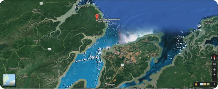
The Alcântara Launch Center is located on the north coast of the state of Maranhão, Brazil (Fig. 1), at the geographic coordinates 2°19’ S, 44°22’ W, 50 msl and at a distance of 30 km from the city of São Luiz, Maranhão. Figure 2 shows the respective localization of the ALC, the Mobile Tower Integration (MTI) where rockets are launched, and the Anemometric Tower (AT) where data are collected to analyze the surface wind profile characteristics. This place is close to the sea and the vegetation is characteristic of restinga, with trees ranging from 2.0 up to 3.0 m height.

(3)

J. Aerosp. Technol. Manag., São José dos Campos, v10, e4318, 2018

EXPERIMENTAL ARRANGEMENTS

CHARACTERISTICS OF THE “PROF. JOAQUIM BLESSMANN” WIND TUNNEL

The tests were performed in the Wind Tunnel (WT) Prof. Joaquim Blessmann. Briefly, it is an enclosed return boundary wind tunnel, specifically designed for static and dynamic testing of civil engineering construction models. The correct simulation of the main characteristics of natural wind in wind tunnels is a basic requirement for applications in Civil Engineering, without which the results obtained can deviate considerably from reality.

Pioneer in Latin America, the WT Prof. Joaquim Blessmann, from the Federal University of Rio Grande do Sul, Porto Alegre, Brazil (Blessmann 1982), has a length/height ratio of the test chamber greater than 10. The velocity of the airflow in this chamber, uniform flow without any models, exceeds 46 m/s. The equipment allows the simulation of the main characteristics of natural winds in the atmospheric boundary layer and allows the correct determination of the working pressures on the facades and structure of the buildings.

Figure 1. Spatial location of the Alcântara Launch Center obtained through satellite image using Google Earth on 07/02/2017 at 9:00 p.m.

Figure 2. (a) Localization; and (b) topographic characteristics of the Alcântara Launch Center (Pires et al. 2015).

(4)

xx/xx 04/17

INCIDENT WIND SIMULATION

In Wind Engineering, the vertical variation of the mean velocity U is usually expressed from the potential law, which is valid throughout the boundary layer. This law is defined by Eq. 1, where U_ref is the reference velocity obtained at the reference height z_ref (usually assumed as 10 m). The exponent α varies from 0.09 to 0.45, depending on the surface roughness of the terrain and the thermal stability. Atmospheric turbulence is characterized by the turbulence intensity Iu, defined by the ratio between the standard deviation of the fluctuations u’ and the mean velocity U. Complementarily, the turbulence spectrum allows to evaluate the energy distribution as a function of frequency. Measurements made in the atmosphere allow evaluation of the atmospheric spectra, which are then used to validate the results obtained in wind tunnels.

(1)

In order to study the aerodynamic phenomena that occur in the atmospheric boundary layer, it is necessary to simulate inside a WT. The simulation process consists of developing a physical model of the atmospheric flow so the characteristic parameters are reproduced in the best possible way inside the tunnel. In most laboratories it is more common to simulate the neutral boundary layer. This implies modeling the distribution of mean velocities, turbulence scales and atmospheric power spectrum (Surry 1982). Counihan (1969) and Standen (1972) employing roughness methods, barrier and blending devices, have developed particularly suitable simulation techniques for reproducing boundary layers under conditions of neutral stability. These techniques allow us to obtain representations of the boundary layers that occur on rural and urban lands. In a previous work, Loredo-Souza et al. (2004) carried out a detailed description of the systems, methodologies and ways of evaluating the physical models of atmospheric flow in a neutrally stable in boundary layer wind tunnels.

According to the characteristics of the roughness of the terrain around the ALC, a wind profile was simulated using a potential profile of mean velocities and exponent α = 0.11 (representative roughness of Category I) according to NBR 6123 (Blessmann 1995). The roughness characteristics of the simulated terrains correspond to a large smooth surface, more than 5 km in length, measured in the direction of the incident wind. The simulators used to simulate the wind characteristics are shown in Fig. 3.

α

a

)

/

(

/

U

_ref

z

_ref

U

₌

Figure 3. Entrance of the wind tunnel and the turbulence generator.

α

0 100 200 300 400 500 600

0.00 0.50 1.00 1.50

z [ m m ] U(z)/U(450) exp. 0,11 0 100 200 300 400 500 600

0.00 5.00 10.00 15.00

z [ m m ] u'/U [%] exp. 0,11 0 100 200 300 400 500 600

0.00 100.00 200.00 300.00

(5)

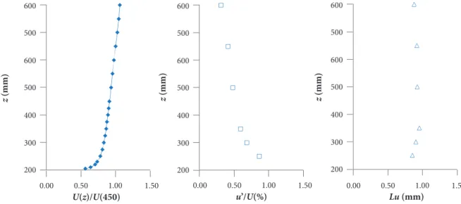
Based on the characteristics of the site under study and the landscape at ALC, it was tested the model for incident winds with these characteristics. Around the model, the closest buildings were reproduced on the scale of the model so that the flow conditions corresponded as closely as possible to the real conditions. The main characteristics of the simulated winds can be seen in Fig. 4, where the vertical profile of the mean velocities U(z)/U(450) is indicated, where U(450) is the mean velocity in the longitudinal axis of the tunnel, the intensity of turbulence u’/U and the macro-scale Lu of the longitudinal component of the turbulence.

Figure 4. Main characteristics of the incident flow (exponent α = 0.11).

600

500

600

500

400

300

200

0.00 0.50 1.00

U(z)/U(450)

z

(mm) z (mm) z (mm)

u’/U(%) Lu (mm)

1.50 0.00 0.50 1.00 1.50 0.00 0.50 1.00 1.50

600

500

600

500

400

300

200

600

500

600

500

400

300

200

CONCENTRATION MEASUREMENTS

The study of dispersion processes based on wind tunnel experiments requires measuring the concentration of a given gas. The measurement system depends on the type of gas used as a tracer and for this work a hot wire anemometer was used combined with an aspirating probe (Wittwer 2006). From the calibration process, the suction probe allows direct determination of instantaneous concentration values for a binary mixture. The gas flows and concentration of the binary mixtures were necessary to correctly simulate the problems and phenomena of dispersion in the wind tunnel, and also to calibrate the instruments of measurement of the concentrations.

To obtain binary mixtures of gases with fixed velocity and flow, it was used the device shown in Fig. 5a. This device was built in the Aerodynamics Laboratory of the Buildings of Universidade Federal do Rio Grande do Sul (UFRGS). The mixture was obtained by two series of small holes of different diameters that work as sonic tubes. Each of the series of holes allows an accurate flow of helium and air, respectively, and with the interconnection at the end of the circuit the exact mixture is obtained. The degree of accuracy of the mixing device depends on the number of sonic tubes and the accuracy with which the orifices are calibrated. The relative errors are larger in the smaller diameter holes, in this case 0.50 mm. The mass concentration (C) corresponds to a mixture of helium (He) and air flows, and it is evaluated by Eq. 2.

(2)

𝐶𝐶 =_𝑄𝑄 𝑄𝑄𝑚𝑚(He)

𝑚𝑚(He) + 𝑄𝑄𝑚𝑚(Ar)

(6)

xx/xx 06/17

the aspiration, causes the sonic blockage. The hot wire thus becomes a sensor that notices the variations of the thermal properties of the fluid in the process of heat transfer, that is, it measures the variations of gas concentration.

The dynamic response of the aspirating probe can be analysed by a constructing concentration spectra. Results obtained for a helium-air coaxial jet using different frequencies of acquisition between 5 and 10 kHz guarantee the dynamic response of this type of probe to frequencies above 1 kHz. The characteristic scales in wind tunnels usually do not require the analysis of frequencies greater than 1 kHz (Loredo-Souza and Wittwer 2010).

Figure 5. (a) Calibration system; and (b) aspirating probe.

(a)

(b)

(a)

(b)

EVALUATION OF THE ALCÂNTARA LAUNCH CENTER ATMOSPHERIC FLOW

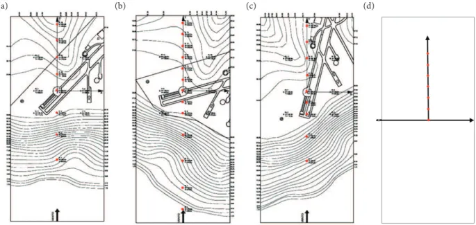
The analysis of the atmospheric flow was based on two important physical characteristics: velocity profiles and fluctuations at different points of interest in the studied region. Figure 6 shows representative models of the three angles of wind incidence analysed, nominally 0°, 30° and 330°. The choice of incidence angles was based on wind directions with ± 30° variability, predominantly, from the marine coast of the ALC region (Gisler et al. 2011).

Figure 6. Models built on reduced scale (1/400) of ALC for the three directions of wind incidence: (a) 0°, (b) 30° and (c) 330°, and (d) the simplified model (Step-like).

(7)

This initial evaluation consisted of studying the atmospheric flow characteristics and gas dispersion processes in the ALC region. The results of the evaluation of the flow in the vicinity of the ALC are presented in a complementary work (Wittwer et al. 2016b) where a quantitative analysis of vertical profiles of mean velocity and turbulence intensity was carried out. In addition, the results were compared with the type of topographic model used in the study for the three directions of wind incident in the WT. Basically, this study allows determining the points where the largest flow variations occur in the vicinity of the surface with respect to the incident flow.

Wittwer et al. (2016b) presented, in a complementary way, the atmospheric flow results obtained with a simplified step-like model (Fig. 6). An interesting conclusion obtained from this evaluation is that simplifications can lead to results that do not reflect the actual situation. Consequently, it is important to emphasize the importance of using topographic models that reproduce the surrounding environment by applying a defined geometric scale according to the scale of the incident wind, in order to obtain reliable results in WT studies.

A previous work was developed by Marinho Pires et al. (2010) where atmospheric flow measurements were carried out using the PIV and HWA techniques on a simplified wind tunnel model of the ALC region constructed with a scale factor of 1:1000. Also, full scale in situ wind measurements using aerovanes and sonic anemometers at Alcântara Launch Center were previously analysed by Fisch (2010). These studies were used to define the 1/400 scale model constructed for the present work and they can be used to translate the results obtained at the scale model to analyse the full-scale problem.

EXPERIMENTAL ANALYSIS OF THE TURBULENT DISPERSION PROCESS

Basically, the topographic model studied is representative of the Alcantara Launch Center, with a 0° angle deviation for the predominant wind direction. However, a complementary measurement was made with the model corresponding to the wind incident in the direction 330°, that is, with a wind direction rotation of 30° (Fig. 7). The preliminary results of the dispersion study use a wind tunnel with reproduction of the atmospheric flow, which were simulated from the small scale models that reproduce the topographic conditions and simulate the atmospheric flow of the ALC region. The dispersion process was evaluated using a hot wire anemometer with an aspirating probe. The dimensionless concentration coefficient K is defined as Eq. 3.

(3)

(4)

0 2

Q H CU

K ref

=

ref C

c c I = ´

where: C is the measured concentration; U_ref is the reference velocity; H is the reference height of 160 m; and Q₀ is the emission flow rate. The intensity of the concentration fluctuations I_cis defined by the ratio of the standard deviation of the fluctuations c’ to the maximum value of the mean concentration at the profile C_ref (Eq. 4).

(8)

xx/xx 08/17

RESULTS FOR EMISSION AT GROUND LEVEL – MODEL 0°

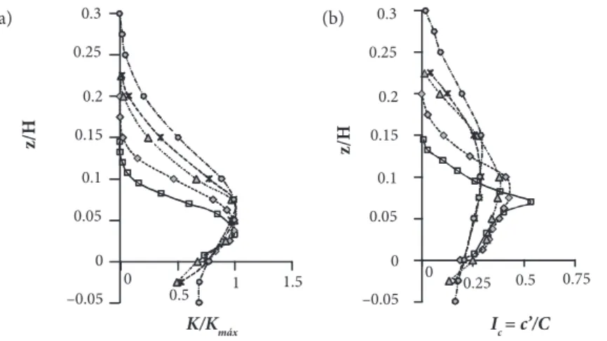
In Table 1 are indicated the characteristics that define the conditions of dispersion of the plume for the ground level emission (A, B, C and D). The measuring locations are indicated in the graphs by the dimensionless coordinates (x/H, y/H). Figure 9 presents the vertical profiles of the non-dimensional mean concentration K/K_m and the intensity of the concentration fluctuations I_c, obtained with emission at the ground level in the leeward positions of the emission, with spacings and /H of 0.25, 0.50, 1.00, 1.50 and 2.25, respectively, for the reference height H = 400 mm. The emitted helium flow rate was 0.176 dm3_{/s and the reference} air velocity is 2.60 m/s, which define condition A for the emission plume as can be seen in Table 1.

Figure 10 shows the vertical profiles of concentration K and intensity I_c obtained with a helium flow rate of 0.703 dm3_{/s and the} same air reference velocity (2.60 m/s), which determine condition B for the emission pen. The leeward positions of the emission are y/H of 0.25, 0.50, 1.00, 1.50, and 2.25, respectively.

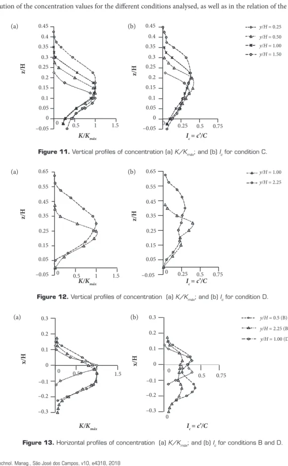
The vertical profiles of concentration K and the intensity of concentration fluctuations I_c corresponding to condition C for the emission plume, obtained with a helium flow of 1.582 dm3_{/s and air velocity of 2.60 m/s, are shown in Fig 11. The locations}

Figure 7. Topographic models developed for two incident wind directions (a) 0°; and (b) 330°.

(b)

(a)

(b) (b)

(9)

evaluated are y/H = 0.50, 1.00, 1.50 and 2.25, respectively. The condition D, defined from an emission of 1,582 dm3_{/s of helium} and an air reference velocity of 1.65 m/s, was analysed in Fig. 12, where the vertical profiles are shown in the leeward positions of the emission at H = 1.00 and 2.25.

Figure 13 presents the horizontal profiles, which allow evaluating the lateral symmetry of the emission plume with only three concentration profiles being evaluated. For condition B of the emission plume, the leeward positions of the emission were evaluated at H = 0.50 and 2.25. In the further leeward position, a displacement of the center of the plume is observed. For condition D, the horizontal profile at the y/H = 1.00 position shows a lateral displacement of the center of the plume similar to that obtained for condition B.

Table 1. Conditions for emission at ground level.

Condition Q0 [dm

3_/s] _w

0 [m/s] Uref [m/s] w0/Uref

A 0.176 0.560 2.60 0.215

B 0.703 2.238 2.60 0.861

C 1.582 5.036 2.60 1.937

D 1.582 5.036 1.65 3.052

0.3 0.25 0.2 0.15 0.1 0.05

0.5 1 1.5 0.25 0.5 0.75

0 0 –0.05

z/H _z/H

0.3 y/H = 0.25

y/H = 0.50

y/H = 1.00

y/H = 1.50

y/H = 2.25 0.25

0.2 0.15 0.1 0.05 0

0 –0.05

K/K

máx Ic = c’/C

0.3 0.25 0.2 0.15 0.1 0.05

0.5 1 1.5 0.25 0.5 0.75

0 0 –0.05

K/K

máx Ic=c’/C

z/H _z/H

0.3 _y/H_{= 0.25}

y/H = 0.50

y/H = 1.00

y/H = 1.50

y/H = 2.25 0.25

0.2 0.15 0.1 0.05 0

0 –0.05

Figure 9. Vertical profiles of concentration (a) K/K

máx; and (b) Icfor condition A.

máx; and (b) Icfor condition B. (a)

(a)

(b)

(10)

xx/xx 10/17

Figure 13. Horizontal profiles of concentration (a) K/K

máx; and (b) Icfor conditions B and D. 0.45 0.4 0.35 0.3 0.25 0.2 0.15 0.1 0.05 0 –0.05 0.45 0.4 0.35 0.3 0.25 0.2 0.15 0.1 0.05 0 –0.05

0.5 1 1.5 0.25 0.5 0.75

0

z/H _z/H

y/H = 0.25

y/H = 0.50

y/H = 1.00

y/H = 1.50

0

K/K

máx Ic = c’/C

0.65 0.55 0.45 0.35 0.25 0.15 0.05 –0.05 0.65 0.55 0.45 0.35 0.25 0.15 0.05 –0.05

0.5 1 1.5 0.25 0.5 0.75

0 0

z/H _z/H

y/H = 1.00

y/H = 2.25

K/K

máx Ic = c’/C

0.3 0.2 0.1 0 –0.1 –0.2 –0.3 0.3 0.2 0.1 0 –0.1 –0.2 –0.3 0.5 1

1.5 _0.5 _0.75

0 0

0

x/H _x/H

y/H = 0.5 (B)

y/H = 2.25 (B)

y/H = 1.00 (D)

K/K

máx Ic = c’/C

"#%'

máx; and (b) Icfor condition C.

Figure 12. Vertical profiles of concentration (a) K/K_máx; and (b) I_cfor condition D.

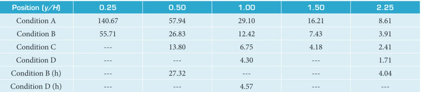
The results are complemented with the values of K_máxindicated in Table 2. These values allow evaluating the dispersion process evolution in terms of the leeward position related to the emission location. In general, the results show consistency with respect to the dilution of the concentration values for the different conditions analysed, as well as in the relation of the distributions of

(11)

the measured values in the leeward positions of the emission and laterally. The measurements were made considering only the incident wind direction corresponding to 0º (perpendicular to the coast).

Table 2. Values of K

máx for emission at ground level – model 0°.

Position (y/H) 0.25 0.50 1.00 1.50 2.25

Condition A 140.67 57.94 29.10 16.21 8.61

Condition B 55.71 26.83 12.42 7.43 3.91

Condition C --- 13.80 6.75 4.18 2.41

Condition D --- --- 4.30 --- 1.71

Condition B (h) --- 27.32 --- --- 4.04

Condition D (h) --- --- 4.57 ---

---It is interesting to observe the similar behavior in the different conditions regarding the configuration of vertical profiles of mean concentration. Regarding the concentration fluctuations, the I_c intensity profiles also show a similar behavior under the different conditions with the exception of the D condition. The general behavior indicates a configuration with smooth variations with a peak of the fluctuations in the position just above the point defining the maximum value in the mean concentration profile. The horizontal profiles of mean concentration show a Gaussian and symmetrical configuration, due to the absence of a lateral limitation. In the case of fluctuation intensities, the profiles define two peaks, approximately at points located at a distance x/H = 0.1 to the left and right of the point corresponding to the maximum value in the mean concentration profile.

RESULTS FOR EMISSION DOWNWARD SIMULATING THE ROCKET – MODEL 0°

The results obtained in the rocket simulation are shown. The survey was performed considering the incident wind direction corresponding to 0º. Table 3 shows the characteristics that define the plume dispersion conditions for emission from top to bottom (E, F, G, H and I).

Table 3. Conditions for emission downward.

Condition Q0 [dm

3_/s] _w

0 [m/s] Uref [m/s] w0/Uref

E 0.176 2.241 2.60 0.862

F 0.703 8.951 2.60 3.443

G 1.582 2.143 2.60 7.747

H 0.176 2.241 1.65 1.358

I 0.703 8.951 4.55 1.967

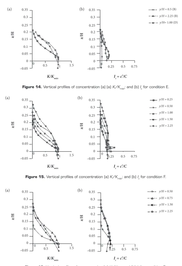
Figure 14 shows the vertical profiles of the non-dimensional mean concentration K and the intensity values of the concentration fluctuations I_c obtained in the leeward positions of the emission, with spacings and /H of 0.25, 0.75 and 2.25 respectively. The helium flow rate was 0.176 dm3_{/s and the reference air velocity is 2.60 m/s, which defines condition E for the emission.}

Figure 15 shows the vertical profiles of concentration K and intensity I_c obtained with an emission of helium of 0.703 dm3_{/s that} determines the condition F for the emission. The leeward positions of the emission are y/H of 0.25, 0.50, 0.75, 1.50 and 2.25, respectively.

(12)

xx/xx 12/17

máx; and (b) Ic for condition G. 0.35 0.3 0.25 0.2 0.15 0.1 0.05 0 –0.05 0.35 0.3 0.25 0.2 0.15 0.1 0.05 0 –0.05

0.5 ₁ 1.5 _0.25 _0.5 _0.75

0

z/H _z/H

y/H = 0.5 (B)

y/H = 2.25 (B)

y/H= 1.00 (D)

K/K

máx Ic = c’/C

0.35 0.3 0.25 0.2 0.15 0.1 0.05 0 –0.05 0.35 0.3 0.25 0.2 0.15 0.1 0.05 0 –0.05

0.5 ₁ 1.5 _0.25 _0.5 _0.75

0

z/H _z/H

y/H = 0.25

y/H = 0.50

y/H = 1.00

y/H = 1.50

y/H = 2.25

K/K

máx Ic = c’/C

0.35 0.3 0.25 0.2 0.15 0.1 0.05 0 –0.05 0.35 0.3 0.25 0.2 0.15 0.1 0.05 0 –0.05

0.5 1.5 _0.25 _0.5 _0.75

0 0

z/H _z/H

y/H = 0.50

y/H = 0.75

y/H = 1.50

y/H = 2.25

K/K

máx Ic = c’/C

Figure 14. Vertical profiles of concentration (a) (a) K/K

máx; and (b) Ic for condition E.

Figure 15. Vertical profiles of concentration (a) K/K_máx; and (b) I_c for condition F.

Figure 18 shows two horizontal profiles corresponding to the F condition of the emission plume obtained in the leeward positions of the emission y/H = 0.25 and 0.75 to evaluate the lateral symmetry of the emission plume.

(13)

Also in this case, the results are complemented with the values of K_máx (Table 4) that allow evaluating the evolution of the dispersion process in terms of the position of the profile. Likewise, the results show consistency with respect to the analysed conditions, and to the distribution of the measured values in the different positions.

Table 4. Values of K

máx for emission downward – model 0°.

Position (y/H) 0.25 0.50 0.75 1.00 1.50 2.25

Condition E 69.78 --- 16.19 --- --- 7.32

Condition F 51.68 24.51 --- 16.68 8.45 5.34

Condition G --- 9.86 7.99 --- 3.11 2.96

Condition H --- --- --- --- --- 5.05

Condition I 110.15 --- --- --- ---

---Condition F (h) 52.71 --- 18.22 --- --- 5.42

Regarding the configuration of vertical profiles of medium concentration, the different conditions show greater differences than in the previous case. The I_cconcentration intensity profiles also do not show a similar behavior under the different conditions.

0.35

0.3

0.25

0.2

0.15

0.1

0.05

0 0.35

0.3

0.25

0.2

0.15

0.1

0.05

0

–0.05 –0.05

1.5

0.5 0.25 0.75

0 ₀

K/K

máx Ic = c’/C

z/H _z/H

y/H = 0.25

y/H = 2.25

0.3 0.2

0.1

0 0 –0.1

–0.2

–0.3

1 1.5

0.5

K/K

máx

x/H

0.3 0.2

0.1

0 0 –0.1

–0.2

–0.3

x/H

0.75 0.5

I

c = c’/C

y/H = 0.25

y/H = 0.75

y/H = 2.25

máx; and (b) Ic for conditions H and I.

Figure 18. Horizontal profiles of concentration (a) K/K

máx; and (b) Ic for condition F. (a)

(a)

(14)

xx/xx 14/17

The general behavior indicates a configuration with smooth variations, but without the clear definition of a peak as it happens in the case of emission at ground level.

The horizontal profiles of mean concentration also do not show a Gaussian symmetrical configuration as in the case of emission at the ground level. In the same way, the profiles of the fluctuation intensities I_c show two peaks, but they are not well defined as it happens in the previous case.

RESULTS FOR EMISSION DOWNWARD SIMULATING THE ROCKET – MODEL 330°

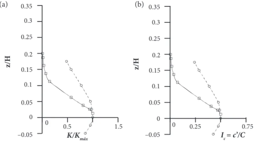
Some results were obtained in the direction corresponding to the incident wind direction at 330°. The vertical profiles of concentration K and the intensity of the fluctuations I_cobtained at the y/H positions of 0.25, 0.75 and 1.50, respectively, for the emission condition F, are shown in Fig. 19. Table 5 indicates the values of K_máxto evaluate the evolution of the concentration profiles.

máx;and (b) Ic for condition F. 0.35

0.3 0.25 0.2 0.15 0.1 0.05 0 0.35

0.3 0.25 0.2 0.15 0.1 0.05 0

–0.05

–0.05 0.5 1 1.5 0.25 0.5 0.75

0 0

K/K

máx Ic = c’/C

z/H _z/H

y/H = 0.25

y/H = 0.75

y/H = 1.50

Table 5. Values of K_máx for emission downward – model 330°.

Position (y/H) 0.25 0.75 1.50

Condition F 58.11 19.42 10.02

DISCUSSION OF RESULTS

Results for emission at ground level presented in Figs. 9 to 13 indicate a Gaussian behavior of the concentration vertical profiles in the upper part of the plume. Some modifications of the profiles are produced in the lower part (close to the floor) with relation to Gaussian behavior. Table 2 indicates a gradual diminution of maximum concentration values from the nearest position of the emission to the far away position. Comparison of vertical profile configurations near the emission with respect to emitted gas volume indicates maximum concentration at ground level with minor emitted gas (condition A), while the maximum concentration in the case of maximum emission (condition C) occurs at z/H = 0.10.

Figures 14 to 18 for emission downward and model 0° show different behaviors according to the emission condition analysed. Differences with relation to Gaussian behavior are more evident in some cases. Results obtained for condition F show values more similar to the results obtained with ground level emission, however, the vertical dispersion is always greater for emission downward cases. At the same time, intensities of concentration fluctuations are always minor than 0.25 in these cases, while the corresponding values for ground level emission are clearly greater.

(15)

General comparison between the plume behaviour for incident wind direction of 0° (Fig. 15) and 330° (Fig. 19) indicates maximum values of concentration a little greater for direction 0°. The same occurs with respect to the values of the fluctuating concentration. This behavior is coherent with the topographic configuration related to each incident wind direction, being that the slope upwind the emission is greater for direction 0°. Previous measurements of atmospheric flow indicated turbulence levels leeward emission greater for the case of wind direction of 330°. So, the mixing process is faster and the dispersion is greater diminishing the concentration fluctuations.

CONCLUSIONS

The work presents the experimental evaluation of the dispersion process at the ALC region. A quantitative analysis of the vertical and horizontal profiles of the mean concentration and fluctuation intensity, and comparisons between results obtained for two incident wind directions were carried out by tests using wind tunnel.

The general comparison between the values obtained for the emission at ground level and for the case of the emission downward indicates greater concentration dilution for the first case. These results are predictable taking into account that the turbulent diffusion can be developed upward, downward and laterally in the case of the ground level emission.

The importance of the incident wind simulation and topographical model are shown in this paper. The use of wind tunnel tests to analyse this type of phenomena is also highlighted.

In general, results obtained with the emission at ground level indicate a similar behavior with previous work (Wittwer et al. 2007b; 2011), and the evolution of the K_máx values are coherent with dilution factor obtained for this type of process (Chui and Wilson 1988; Saathoff et al. 1998). Similar experimental studies considering the case of the emission downward are not found in the specific literature, but the obtained general behavior and the measured values showed coherence with respect to the case of the emission at ground level. A multilayer model to simulate rocket exhaust clouds was developed by Moreira et al. (2011) and further simulations to analyse dispersion process using this model will permit to complete this experimental study.

AUTHOR’S CONTRIBUTION

Conceptualization, Wittwer A, Loredo-Souza A and Oliveira M; Methodology, Wittwer A, Loredo-Souza A and Oliveira M; Investigation, Wittwer A, Loredo-Souza A, Oliveira M, and Souza B; Writing – Original Draft, Wittwer A, Loredo-Souza A, Oliveira M, Fisch G and Goulart E; Writing – Review and Editing, Souza B.

Blessmann J (1982) The boundary layer tv-2 wind tunnel of UFRGS. Journal of Wind Engineering and Industrial Aerodynamics 10(2):231-248. doi: 10.1016/0167-6105(82)90066-6

Blessmann J (1995) O vento na engenharia estrutural. Porto Alegre: Editora da Universidade, UFGRS.

Cao S, Tamura T (2006) Experimental study on rounghness effects on turbulent boundary layer flow over a two-dimensional steep hill. Journal of Wind Engineering and Industrial Aerodynamics 94(1):1-19. doi: 10.1016/j.jweia.2005.10.001

Chui EH, Wilson DJ (1988) Effect of varying wind direction on exhaust gas dilution. Journal of Wind Engineering and Industrial Aerodynamics 31(1):87-104. doi: 10.1016/0167-6105(88)90189-4

Counihan J (1969) An improved method of simulating an atmospheric boundary layer in a wind tunnel. Atmospheric Environment 3(2):197-214. doi: 10.1016/0004-6981(69)90008-0

Degrazia GA, Anfossi D, Carvalho JC, Mangia C, Tirabassi T, Campos Velho HF (2000) Turbulence parameterisation for PBL dispersion models in all stability conditions. Atmospheric Environment 34(21):3575-3583. doi: 10.1016/S1352-2310(00)00116-3

(16)

xx/xx 16/17

Delaunay D, Lakehal D, Barré C, Sacré C (1997) Numerical and wind tunnel simulation of gas dispersion around a rectangular building. Journal of Wind Engineering and Industrial Aerodynamics 67-68:721-732. doi: 10.1016/S0167-6105(97)00113-X

Faria AF (2016) Análise experimental do escoamento atmosférico no Centro de Lançamento de Alcântara utilizando túnel de vento (Master’s Dissertation). São José dos Campos: Instituto Tecnológico de Aeronáutica. In Portuguese.

Fisch G (2010) Comparisons between aerovane and sonic anemometer wind measurements at Alcântara Launch Center. Journal of Aerospace Technology and Management 2(1):105-110. doi: 10.5028/jatm.2010.0201105110

Gisler CAF, Fisch G, Correa CDS (2011) Análise estatística do perfil de vento na camada limite superficial no Centro de Lançamento de Alcântara. Journal of Aerospace Technology and Management 3(2):193-202. doi: http://10.5028/JATM.2011.03022411

Harion J, Camano E, Favre-Marinet M (1995) Mesures de vitesse et de concentration par thermo-anémométrie dans des mélanges air/ helium. C R Acad Sci Paris 320(2):77-84.

Jensen NO, Busch NE (1982) Atmospheric Turbulence. Amsterdam: Elsevier.

Kastner-Klein P, Plate EJ (1999) Wind-tunnel study of concentration fields in street canyons. Atmospheric Environment 33(24-25):3973-3979. doi: 10.1016/S1352-2310(99)00139-9

Loredo-Souza AM, Schettini EBC, Paluch MJ (2004) Simulação da camada limite atmosférica em túnel de vento. Presented at: IV Escola da Primavera Transição e Turbulência. Anais da IV Escola da Primavera Transição e Turbulência; Porto Alegre, Brazil.

Loredo-Souza AM, Wittwer AR (2010) Estudo em Túnel de Vento do Processo de Disperssão de Gases no Centro de Lançamento de Alcântara. Technical Report. Laboratório de Aerodinâmica das Construções.

Magnago R, Fisch G, Moraes O (2008) Análise Espectral do Vento no Centro de Lançamento de Alcântara (CLA). Revista Brasileira de Meteorologia 25(2):19.

Marinho Pires LB, Roballo S, Fisch G, Avelar A, Girardi R, Gielow R (2010) Atmospheric flow measurements using the PIV and HWA techniques. Journal of Aerospace Technology and Management 2(2):127-136. doi: 10.5028/jatm.2010.02027410

Marvoidis I, Griffiths JS, Hall DJ (2003) Field and wind tunnel investigations of plume dispersion around single surface obstacles. Atmospheric Environment 37(21): 2903-2918. doi: 10.1016/S1352-2310(03)00300-5

Meroney RN, Leitl BM, Rafailidis S, Schatzmann M (1999) Wind-tunnel and numerical modeling of and dispersion about several building shapes. Journal of Wind Engineering and Industrial Aerodynamics 81(1-3):333-345. doi: 10.1016/S0167-6105(99)00028-8 Moreira DM, Trindade LB, Fisch G, Moraes MR, Dorado RM, Guedes RL (2011) A multilayer model to simulate rocket exhaust clouds. Journal of Aerospace Technology and Management 3(1):41-52. doi: 10.5028/jatm.2011.03010311

Novak MD, Wardland JS, Orchansky AL, Ketler R, Green S (2000) Wind tunnel and field measurements of turbulence flow in forests. Part I: uniformly thinned stans. Boundary Layer Meteorology 95(3):457-495. doi: 10.1023/A:1002693625637

Pires LBM, Fisch G, Gielow R, Souza LF, Avelar AC, Paula IB, Girardi R (2015) A study of the internal boundary layer generated at the Alcantara Space Center. American Journal of Environmental Engineering 5(1A):52-64. doi: 10.5923/s.ajee.201501.08

Roballo ST, Fisch G (2008) Escoamento atmosférico no Centro de Lançamento de Alcântara (CLA): Parte I - aspectos observacionais. Revista Brasileira de Meteorologia 23(4):510-519.

Saathoff P, Stathopoulos T, Wu H (1998) The influence of the freestream turbulence in nearfield dilution of exhaust from building vents. Journal of Wind Engineering and Industrial Aerodynamics 77-78:741-752. doi: 10.1016/S0167-6105(98)00188-3

Schuch D, Fisch G (2017) The use of an atmospheric model to simulate the rocket exhaust effluents transport and dispersion for the Centro de Lançamento de Alcântara. Journal of Aerospace Technology and Management 9(2):137-146. doi: 10.5028/jatm.v9i2.740 Standen NM (1972) A Spire Array for Generating Thick Turbulence Shear Layers for Natural Wind Simulation in Wind Tunnels. (LTR-LA-94). NAE Technical Report.

Surry D (1982) Consequences of distortions in the flow including mismatching scales and intensities of turbulence. Presented at: International Workshop on Wind Tunnel Modeling Criteria and Techniques in Civil Engineering; Gaithersburg, USA.

Wittwer AR (2006) Simulação do vento atmosférico edos processos de dispersão de poluentes em túnel de vento (PhD Thesis). Porto Alegre: Universidade Federal do Rio Grande do Sul. In Portuguese.

Wittwer AR, Loredo-Souza AM, Schettini EBC (2007a) Avaliação das flutuações de concentração em uma pluma de dispersão de poluentes. Ciência e Natura Edição especial:141-144.

(17)

Wittwer AR, Loredo-Souza AM, Schettini EBC (2011) Laboratory evaluation of the urban effects on the dispersion process using a small-scale model. Presented at: 13th International Conference on Wind Engineering. Proceedings of the ICWE13; Amsterdam, The Netherlands.

Wittwer AR, Loredo-Souza AM, Oliveira MGK, Souza BH, Fisch G, Goulart EV (2016a) Estudo do processo de dispersão turbulenta de gases no Centro de Lançamento de Alcântara. Presented at: 10th ABCM Spring School on Transition and Turbulence; São José dos Campos, Brazil.

Wittwer AR, Loredo-Souza AM, Oliveira MGK, Souza BH, Fisch G, Goulart EV, Carvalho GF (2016b) Simulação das características do vento atmosférico no Centro de Lançamento de Alcântara. Presented at: 10th ABCM Spring School on Transition and Turbulence; São José dos Campos, Brazil.