Computer simulation of rapid solidification with undercooling: A case study of spherical ceramics sample on metallic substrate

_____________________________

*) _{Corresponding author: [email protected]}

doi:

10.2298/SOS1001033N

UDK 662.785:519.001.573

Computer Simulation of Rapid Solidification With

Undercooling: A Case Study of Spherical Ceramics Sample

on Metallic Substrate

Z. S. Nikolic

1*)

, M. Yoshimura

2

1

Faculty of Electronic Engineering, Department of Microelectronics

University of Nis, 18000 Nis, PO Box 73, Serbia

2

Tokyo Institute of Technology, Materials and Structure Laboratory

Yokohama 226-8503, Japan

Abstract:

Generally speaking, complex rapid solidification process kinetics can be solved by using numerical techniques only. In that sense, numerical methods for simulation of the solidification processes can be categorized as fixed-grid and interface tracking schemes, where the former ones cannot accurately track a sharp solid-liquid interface. Therefore, in this paper a numerical method based on control volume methodology and interface-tracking technique for computer simulation of rapid solidification accompanied by melt undercooling will be described and applied to analyze the solidification of a ceramic sample on a metallic substrate. A digital pyrometry system will be used for temperature measurement in an Arc-image furnace because of its merit of presenting data directly as temperature in real time with high accuracy. The characterization of solidification of a ceramic sample will be done by using the defined numerical method and inverse heat transfer analysis.

Keywords: Rapid solidification, Computer simulation

Introduction

Oxide ceramics have good intrinsic properties such as oxidation resistance, chemical and thermal stability, but also poor resistance to thermal shock and in general to crack propagation and growth, which results in rapid material degradation and catastrophic fracture. One way to improve the thermo-mechanical stability of ceramic oxide composites is their fabrication by solidification from eutectic melt [1]. Eutectic composites fabricated by unidirectional solidification have excellent strength and creep resistance at high temperature [2]. The strengthening of grain boundaries characteristic of eutectics is especially required for long-term service in high temperature applications [3]. However, the fabrication of oxide eutectics by more rapid solidification techniques has yielded moderate success, producing partially amorphous or inhomogeneous samples, because it is difficult to maintain a homogeneous heat transfer at high cooling rates [4-9]. Rapid solidification methods have been used to fabricate eutectic powders, but not layered eutectic crystals.

To get rapidly quenched samples of high temperature materials, many techniques have been developed. Some of them, such as splat cooling, melt-spinning, spray deposition and strip casting are based on bringing the melt in intimate contact with a substrate. However, rapid solidification is not easily accessible experimentally due to the simultaneously small time and spatial scales. Especially because of the high cooling rates realized it is difficult to measure the relevant process parameters. Therefore attempts have been made to calculate the operating conditions for the formation of crystalline and amorphous alloys from heat transfer models. In that sense, tracking the interface location accurately can be provided by modified fix-grid schemes, such as, for example, the node-jumping scheme [11] or the element subdivision method [12]. Recently Nikolic et al. [13] adopted a numerical model to analyze heat transfer process during solidification of sample melted in an Arc-image furnace [14,15], in which the melt cooling rate and the solidification rate are controlled by the interfacial heat transfer conditions between spherical sample and colder substrate, and where the governing heat conduction equations for solidifying sample and substrate as a heat sink were derived assuming spherical symmetry. Combining control volume methodology [16] and the interface-tracking technique Nikolic and Yoshimura [17] described a finite difference method for simulation of solidification (with and without undercooling) of a sample on a substrate, which was applied for thermal history analysis in both sample and substrate, including the phase change phenomena. It was shown that such an approach can be used for investigation of solidification experimentally and numerically [18]. In this paper we will describe in detail a numerical method based also on control volume methodology for simulation of solidification with melt undercooling for a heat-transfer model spherical sample on a metallic substrate. This approach will be applied for thermal history analysis of alumina sample solidified on copper substrate.

2. Mathematical model

We will define a two-dimensional (2-D) heat transfer model by considering solidification of the solid spherical sample on the solid substrate cooled by water. This problem exhibits symmetry about an axis of rotation and can be solved using a 2-D approach. Namely, this radially symmetric heat-conduction problem will be solved numerically by assuming a nonuniform temperature distribution inside the sample, and symmetric about the growth axis, which coincides with the substrate-sample direction. In this approach multi-dimensional effects are believed to be small for cooling and solidification processes.

The governing heat conduction equations, assuming constant conductivity, can be written as

t y x T c

y y x T

x y x

T _p

p p p p

p

∂ ∂ =

∂ ∂ + ∂

∂ ( , ) ( , ) ( , )

λ

ρ

2 2 2

2

(1)

where T is temperature,

ρ

is the density, c is the specific heat capacity,

λ

is the thermal conductivity, t is time, and the subscript

p

=

1

,

2

or

3

represents melt, solid and substrate, respectively. For numerical solution of equation (1) we will assume that the rectangular experimental region is replaced by a finite difference mesh defined by grid spacings Δx and

sam n k

sam k sam

D

,..., 2 , 1

} CV

{ ₌

=

sub n k

sub k sub

D

,..., 2 , 1

} CV

{ ₌

= ,

where n_sam and n_sub are the numbers of CVs for the sample and the substrate, respectively, represents the complex sample-substrate domain of a heat transfer problem to be solved.

Introduction of domain methodology will allow us to track the interface across the neighboring CVs in horizontal and vertical directions inside the sample with increased interface tracking resolution. The mathematical model for interface tracking will be similar to the approach of Wang and Matthys [12] but adopted for a spherical sample-substrate solidification model and to track the location of the curved interface solid-liquid between CVs of different state as well as across CVs that represent a solid or liquid phase.

The solidification process itself will be divided into three stages: (i) superheated melt (liquid) cooling, (ii) melt solidifying, and (iii) solidified sample cooling. At the beginning of the solidification process, the sample and the substrate are assumed to be at uniform temperatures T_o and T_sub, respectively and the ambient at temperature T_amb.

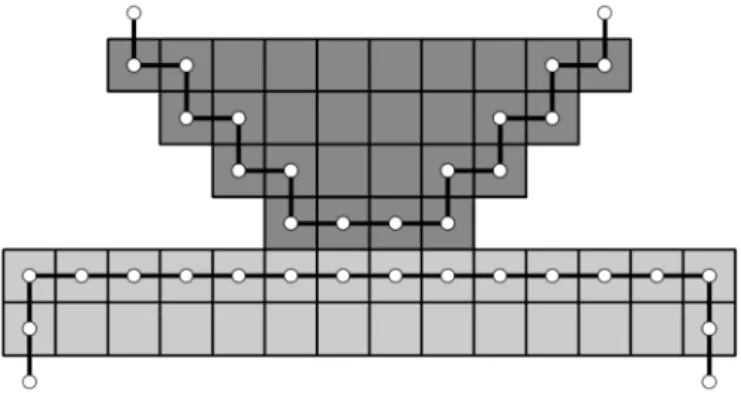
Fig. 1. Sketch of the sample (dark gray) on the substrate (gray), both represented by CVs, where the boundary CVs are marked by open circles (grid points at the center of CVs) and connected by a black line.

For an approximate solution of equation (1) on interior CVs of the sample and the substrate, the explicit method [19] will be used. Since there is no heat source inside the sample, its surface temperature starts to decrease due to heat transfer from the sample to the colder substrate and to the ambient. If the thermal contact between the sample and the substrate is quantified by an interfacial heat transfer coefficient h defined as heat flux through the interface from the sample to the substrate, and if 〈T_sam〉 and 〈T_sub〉 are the average temperatures of the sample and the substrate at the contact interface, respectively, then the temperature at the interface can be computed by equations

) (

) , (

sub sam

I

〉 〈 − 〉 〈 ⋅ = ∂

∂

− h T T

y y x T_p

p

λ ,

where the subscript p=1,2,3 has the same meaning as in equation (1).

However, the boundary CVs of the sample surface will be exposed to some convection boundary condition. Thus, the temperature at the sample surface will be computed differently than on interior CVs. In that sense, the temperature at the sample surface can be computed using corresponding nodal energy balance equations [19], in which the Biot number defined in the finite-difference form as

λ Δx h

provides a measure of the internal conduction resistance relative to the external heat transfer resistance, where h_c is the convective heat transfer coefficient. In our approach we will replace the Biot number definition (2) by an effective Biot number using the combined heat transfer coefficient defined as a sum of the convective (h_c) and the radiative (h_r) heat transfer coefficients, i.e.

amb 4 amb 4

c r c

) , (

) , (

σ ε

T y x T

T y x T h

h h

− − +

=

+ ,

where ε is the total hemispherical emissivity and σ is the Stefan-Bolzmann constant.

Let us assume that the interface substrate-sample is stable through the entire solidification process and that the solidification starts at time t_n on the sample bottom surface across the contact interface with the substrate at the nucleation temperature T_n. During this process the interface starts to change from an initial liquid-solid contact to a solid-solid contact. After that the liquid-solid interface position will be defined by the local equilibrium condition at the solid-liquid interface

I I

s s I s

) , ( )

, (

y y x T y

y x T L

v

∂ ∂ − ∂ ∂

= l

l

λ λ

ρ ,

where T_l and T_s are the temperatures of the melt and solid phase, respectively, L is the latent heat of solidification, and

dt dw v_I =

is the velocity of the solid-liquid interface, where w is the thickness of the solidified layer.

(a) (b)

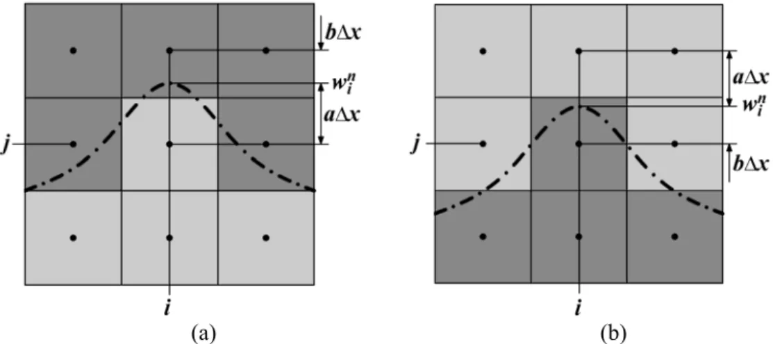
Fig. 2. Two possible interface shapes and locations as well as configurations of solid (gray) and liquid (dark) CVs during solidification near to the sample bottom (a), and to the sample top (b). Interface is drawn by black dashed-dot line.

For solidification with melt undercooling it is convenient to assume that the interface recalesces to the equilibrium melting point after nucleation at time t1 [20]. Since the interface

solid-liquid positions are dictated by the undercooling, for small to moderate undercooling the interface velocity can be related to the interface undercooling

) ( I m T k

T T = − Δ

by the linear kinetics relationship [20] T

where μ_m is the linear kinetic coefficient and T_I(k) is the interface temperature in direction k.

If T_In_(k) is the interface temperature at the previous time step, then the new interface position in direction k will be determined from the equation

t v w

w_kn+1= _kn+ _In_(k)Δ , (3)

where the interface velocity

v

_In_(k) is determined by the interface temperature

T

_In_(k), i.e. )

( _{m I( )}

m ) ( I n k n

k T T

v =μ − .

(a) (b)

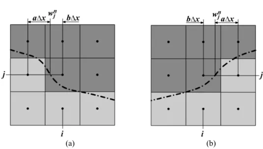
Fig. 3. Two possible interface shapes and locations as well as configurations of solid (gray) and liquid (dark) CVs during solidification along the left (a) and the right (b) sample surfaces. Interface is drawn by black dashed-dot line.

If T_i,jn =Tn(x_i,y_j) is the temperature of CV(x_i,y_j) at the previous time step, the new

temperature distribution in the sample will be now computed by solving the full system consisting of implicit schemes for numerical solution of equation (1) and for the interface nodes L v T x b T x a T x b x a n i n j i n j i n

i s I()

1 , 1 , 1 , s , s 1 ) ( I s ρ Δ λ Δ λ Δ λ Δ

λ _{− − =}

⎥⎦ ⎤ ⎢⎣ ⎡ ₊ + + +

+ l l

l _,

where aΔx and bΔx (

Δ

x

=

Δ

y

) are the distances between the interface position (

w

_in) and the centers of solidified CV and liquid _i,j CV_i,j+1 (Fig. 2a), respectively, and will be determined by equation (3) for k=i. Similar equation will be written for the interface between solidified CV_i−1,j and liquid CV (Fig. 3a) _i,j

L v T x b T x a T x b x a n j n j i n j i n

j s I( )

1 , , 1 , s , 1 s 1 ) ( I s ρ Δ λ Δ λ Δ λ Δ λ = − − ⎥⎦ ⎤ ⎢⎣ ⎡ ₊ + + −

+ l l

l

and between CV_i+1,j and liquid CV (Fig. 3b) _i,j

L v T x b T x a T x b x a n j n j i n j i n

j s I( )

1 , , 1 , s , 1 s 1 ) ( I s ρ Δ λ Δ λ Δ λ Δ λ = − − ⎥⎦ ⎤ ⎢⎣ ⎡ ₊ + + +

+ l l

l _.

(Fig. 2b) we will apply the implicit equation

L

v

T

x

b

T

x

a

T

x

b

x

a

n i n

j i n

j i n

i ( )

, , ,

, )

( s 11 1 s I

s 1 I

s

λ

λ

λ

ρ

λ

₌

Δ

−

Δ

−

⎥⎦

⎤

⎢⎣

⎡

Δ

+

Δ

+ ++ +

l l

l _.

At time t₂ all CVs in the sample will be solidified and the time-dependent temperature distribution T(x,y,t) inside the sample will be computed by the implicit scheme of equation (1) applying corresponding simulation parameters for the solid phase only.

3. Results and discussion

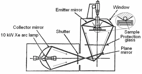
To get rapidly quenched samples of high temperature materials, many techniques (for example [21-23]) have been developed. However, these methods have been limited by factors in maximum temperatures, atmospheres, containers and/or cooling rates. An Arc-Image furnace [14,15] can heat any samples, conductors or insulators, rapidly to a very high temperature in a clean condition, without containers or crucibles, in any atmospheres of oxidizing, inert or reducing. In addition, this furnace has small thermal inertia and great heat concentration at the focus (arc image). These merits provide advantages to the image furnace for rapid heating and quenching of small samples. A detailed description of this method has been given elsewhere [24,25] and only a brief summary will be presented here. Pellets of the mixed powders with the eutectic composition will be placed on a copper plate cooled by water and melted in air in an arc-image lamp furnace (Fig. 4) by the radiation of a Xe lamp (Ushio UF-100001). The spherical arc-melted specimens will be quenched by rapidly moving the copper plate from the focal point. The cooling rate using such method was estimated to be higher than 103 Ks-1 [25].

Fig. 4. Optical system of the arc-imaging furnace

Our model-experiment will be an alumina sample of the diameter 0.003 m placed onto a Cu substrate of the diameter 0.05 m with an assumed substrate-sample circular contact surface of the diameter 0.001 m during solidification. For the initial temperature of the sample we will assume the melt to be superheated uniformly by 2545 K (T_m +218K), and for the substrate and the ambient uniform temperatures 308 K and 300 K, respectively. The values of thermophysical properties used in the simulation will be taken from [27].

method can be used for estimation of the interfacial heat transfer coefficient and for characterization of the solidification process itself. It should be noted that the accuracy of this inverse heat transfer problem solution depends on the accuracy of the applied method for recording the cooling curve. The latter case will be considered bellow for characterization of solidification of alumina by determination of the best matching cooling curve, time-dependent solid-liquid interface profiles and temperature distribution inside the sample.

The previously developed digital pyrometry system with a silicon photocell (with a response time of less than 1 ms) for an arc-image furnace can be used for recording temperature data in which a monochromatic radiation pyrometer was specially designed to measure the radiation temperature of a small specimen at wave-length of 0.65 μm in the temperature range 1200ºC to 3000ºC. The digital pyrometry system used for temperature measurement in the imaging furnace has the merit of presenting with high accuracy every piece of data directly as temperature in real time. A detailed description of this system has been given elsewhere [26]. We will apply this system for recording the temperature history during solidification of alumina on copper substrate.

Oxide materials, on which a larger kinetic effect during undercooling can be expected, have rarely been investigated. In paper [28] rapid solidification of Y3Al5O12 from a

hypercooled melt was carried out. It was shown that the growth velocity of the solid-liquid interface obtained experimentally is in the order of ~ 0.05 ms-1 and proportional to the undercooling throughout the entire undercooling range. By fitting experimental data the linear kinetic coefficient was estimated to be 3.5×10−5m sK. It was also concluded that such a small kinetic coefficient leads to a large kinetic effect even in the low undercooling range. However, the obtained growth velocity was much lower than those of other oxides such as for example alumina. Therefore, in our computation we assumed a higher value for this coefficient,

μ

_m =0.001m sK.

Fig. 5. Matching of numerical prediction (dashed line) with experimental cooling curve (solid line) for alumina on Cu substrate. The melting point (Tm) and characteristic times tn, t1 and t2

are indicated by the dotted lines.

temperature decreased to the nucleation temperature. Crystallization released the heat of fusion and reheated the specimen to the recalescence temperature (T_m). As one can see, a good match between the prediction and measurement is achieved using ΔT =50K,

K W/m

830 2

=

h , Kh_c=570 W/m2 . Weber et al. [29] have investigated solidification of alumina from undercooled melts but by using levitation and laser heating techniques in containerless experiments. The cooling curve was obtained by optical pyrometry. The degree of undercooling which was determined from the cooling curve was dependent on the atmosphere applied. Undercooling of alumina materials (superheated up to 2700 K) was 360 K in an oxygen atmosphere and 450 K in an inert, argon atmosphere. However, it is known that this technique allowed a much larger superheating and undercooling of the liquid.

(a) (b)

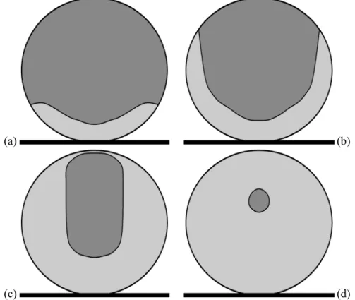
(c) (d)

Fig. 6. Numerical predictions of interface profile at time (a) 0.57 s, (b) 0.65 s, (b) 1.20 s (just after the sample top has solidified), and (c) 1.64 s. (just before the sample being full solidified). Gray and dark gray colored regions are solid and melt, respectively and black bold line is the substrate top.

As it can be seen solidification started at t_n =0.559s when the sample bottom surface reached the nucleation temperature T_n =T_m −ΔT. After that the solidification front moved into a supercooled melt (Fig. 6a), where the melt itself absorbed most of the latent heat and the recalescence took place (Δt_R =51ms). After recalescence, the sample should be cooled down slowly. However, due to convection and radiation solidification of lateral sample surfaces occurred too with developed concave solidification front with thick lateral solidified layers (Fig. 6b). At the same time the sample interior was still at temperature above or very close to the melting temperature. The solidification of lateral sides continued up to

s 197 1

1= .

sample surface. Fig. 5d shows the interface profile just before the end of solidification (t₂=1.664s). The total solidification time (Δt = t2 −tn) was 1.105 s. After that the solidified

alumina sample continued to cool down only.

A considerable change has been observed in the cooling curve of the alumina sample at time t₁=2.05s. In our opinion it might be caused by the change in the heat transfer coefficient at the surface of the sample. Namely, the heat transfer coefficient for a random (turbulence) flow of air must be higher than that for a laminar flow of air. The latter one might be caused by a large difference of temperature between sample surface and ambient air. For this late stage of solidification a good match was obtained for the convective heat transfer coefficient of h_c=100 W/m2K.

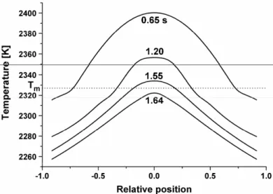
Fig. 7 shows the time-dependent temperature profiles in the horizontal direction across the center of the sample during solidification. The main solidification process occurs in the growth axis direction substrate-sample due to the heat transfer through the sample-substrate contact interface. At 0.65 s the melt cools down continuously with a developed concave like solidification front, the lateral surfaces have already solidified (thick lateral solidified layers shown in Fig. 6b) bellow the melting temperature, whereas the middle of the sample is just bellow the initial temperature, To. At 1.20 s, just after the sample top solidified, the sample middle is now at lower temperature but still liquid. This process continues up to 1.50 s when the sample middle solidifies, whereas at 1.64 s a small amount of melt exists only above the sample center. Full solidification of the sample takes place at 1.664 s and single phase cooling down continues. It can be seen that during solidification the thermal gradient near the sample center is small (almost approaches zero from the macroview), whereas near the sample surface the temperature is lower and is characterized by a steeper temperature gradient due to thermal radiation and convection.

Fig. 7. Time-dependent temperature distribution inside an alumina spherical sample along the diameter direction parallel to the substrate. The numbers -1 and 1 indicate two opposite positions at the sample surface and 0 stands for the center of the sample. The melting point (Tm) is indicated by the dotted line.

4. Conclusion

allowed us to track the solid-liquid curved interface across neighboring CVs of different phases in both horizontal and vertical directions. Assuming that the interface configuration sample-substrate is stable during the entire solidification process, we have defined a 2-D finite difference heat transfer model with a moving solid-liquid interface for solidification with melt undercooling. This method has been applied as a temperature matching method for thermal analysis of rapid solidification of a ceramic (alumina) sample on a copper substrate. A digital pyrometry system has been used for temperature measurement in an Arc-image furnace because of its merit of presenting data directly as temperature in real time with high accuracy. The characterization of solidification of alumina sample has been done using the previously defined numerical method for inverse heat transfer analysis. A very good match between experimental and theoretical results was achieved for the degree of undercooling of 50 K and using the values 830 W/m2K and 570 W/m2K for the interfacial and convective heat transfer coefficients, respectively.

Acknowledgements

The first author performed the present work under a project (No. 142011G) supported financially by the Ministry of Science and Technological Development of the Republic of Serbia. The first author would also like to thank the Japan Society for the Promotion of Science (Invitation Fellowship No. L-06544).

References

1. Y. Waku, N. Nakagawa, T. Wakamoto, H. Ohtsubo, K. Shimizu, Y. Kohtoku, Nature 389 (1997) 49.

2. V. S. Stubican, R. C. Bradt, Ann. Rev. Mater. Sci. 11 (1981) 267.

3. T. Mah, T.A. Parthasarathy, L.E. Matson, Ceram. Eng. Sci. Proc. 11 (1990) 1617. 4. Y. N. Vil'k, E. A. Il'in, A. Y. Timofeev, S. S. Semenov, V. S. Niss, Y. G. Alekseev,

V. N. Kovalevskij, Ogneupory 5 (1992) 11.

5. S. N. Lakiza, A. V. Shevchenko, Z. A. Zaitseva, Y. A. Knysh, Poroshkovaya Metallurgiya (Kiev) 1 (1990) 4.

6. J. McKittrick, G. Kalonji, Mater. Sci. Eng. A231 (1997) 90.

7. J. McKittrick, G. Kalonji, T. Ando, J. Non-Cyst. Solids 94 (1987) 163. 8. N. Claussen, G. Lindemann, G. Petzow, Ceram. Int. 9 (1983) 83. 9. F. P. Glasser, X. Jing, Br. Ceram. Trans. 91 (1992) 195.

10. T. R. Anantharaman, C. Suryanarayana, J. Mater. Sci. 6 (1971) 1111. 11. S. Sundarraj, V. R. Voller, Int. J. Heat Mass Transfer 36 (1993) 713.

12. G.-X. Wang, E. F. Matthys, Int. J. Heat Mass Transfer, 35 [1] (1992) 141-153. 13. Z. S. Nikolic, M. Yoshimura, S. Araki, Mater. Sci. Forum 494(2005)381.

14. T. S. Laszlo, Image Furnace Techniques: Technique of Inorganic Chemistry, Vol. V, Inter-Science Publishers, New York, 1965.

15. M. Yoshimura, J. Coutures, M. Foex, J. Mater. Sci. Lett. 12 (1977) 415.

16. Handbook of Numerical Heat Transfer, Eds. W.J. Minkowycz, E.M. Sparrow, G.E. Schneider, R.H. Pletcher, Wiley, New York, 1988, p. 68.

17. Z. S. Nikolic, M. Yoshimura, J Mater Sci 42 (2007) 7729. 18. Z. S. Nikolic, M. Yoshimura, Key Eng. Mater. 352 (2007) 13.

19. F. P. Incropera, D. P. DeWitt, Introduction to Heat Transfer, John Wiley & Sons, New York, 2002.

21. P. Duwaz, R. H. Willens, Trans. Met. Soc. AIME, 227 (1963) 362. 22. P. T. Sarjeant, R. Roy, J. Amer. Ceram. Soc., 50 (1967) 500. 23. H. Matya, B. C. Giessen, N. J. Grant, J. Inst. Metals, 96 (1968) 30. 24. J.M. Calderon-Moreno, M. Yoshimura, Scripta Mat., 44 (2001) 2153.

25. M. Yoshimura, S. Somiya, in: “4th Intern. Conf. on Rapidly Quenched Metals”, Eds. T. Masumoto, K. Suzuki, Japan Institute of Metals, Sendai, Japan, 1981, pp. 23-26

26. T. Yamada, M. Yoshimura, S. Somiya, High Temp.-High Press. 18 (1986) 377. 27. Information on http://www.ceramics.nist.gov/srd/summary/scdaos.htm.

28. K. Nagashio, K. Kuribayashi, Acta mater. 49 (2001) 1947.

29. J. K. R. Weber, C. D. Anderson, D. R. Merkley, P. C. Nordine, J. Am. Ceram. Soc., 78 [3] (1995) 577.

Са р а: Г

,

. fixed-grid

ђ - . interface tracking .

. interface tracking

.

. З . Arc-image

,

. К

ђ .

.