Rui Pedro Sousa Varandas
Bachelor Degree in Biomedical Engineering Sciences
Evaluation of spatial-temporal anomalies in the
analysis of human movement
Dissertation submitted in partial fulfillment of the requirements for the degree of
Master of Science in Biomedical Engineering
Evaluation of spatial-temporal anomalies in the analysis of human movement
Copyright © Rui Pedro Sousa Varandas, Faculty of Sciences and Technology, NOVA Uni-versity of Lisbon.
The Faculty of Sciences and Technology and the NOVA University of Lisbon have the right, perpetual and without geographical boundaries, to file and publish this disserta-tion through printed copies reproduced on paper or on digital form, or by any other means known or that may be invented, and to disseminate through scientific reposito-ries and admit its copying and distribution for non-commercial, educational or research purposes, as long as credit is given to the author and editor.
This document was created using the (pdf)LATEX processor, based in the “novathesis” template[1], developed at the Dep. Informática of FCT-NOVA [2].
A c k n o w l e d g e m e n t s
With the conclusion of this phase of my life, I would like to acknowledge every person who made it possible.
Firstly, I would like to thank my advisor, Professor Hugo Gamboa of FCT-NOVA, for the guidance, support and exigence during the course of this project. I thank especially for all help provided in times of doubt, for guiding my focus in the right direction and for all the suggestions and opinions given throughout this time. I also thank the chance to learn more about machine learning and signal processing techniques and the inspiration to constantly research and learn more about these topics.
I would also like to thank Fraunhofer Portugal for giving me the opportunity to work in its offices and providing me with all the tools necessary to develop this research. The
working environment was always helpful and the chance to contact with a research en-vironment in such an early stage of my life was excellent for acquiring knowledge about working practices and the challenges and rewards of research work. I am truly grateful to everyone at Fraunhofer Portugal for being so accessible in times of need and especially to Duarte Folgado, without whom this thesis would not be possible. I appreciate all the patience, recommendations and, specially, minutia analysis of every question I made, complex or not. I would also like to thank Marília Barandas for always facilitating and helping with everything was necessary throughout this time. Furthermore, I thank the students team that accompanied me in this laborious task for making it easier, for all help and for the laughs. You were truly outstanding!
To my friends, I thank the hours spent studying, for new insights and motivation, for the time spent playing table football and for all the jokes. Thank you all for the support and help during the last years.
I would like to express my gratitude towards my grandparents who always encour-aged me to keep going in order to be a better person. For all the stories and smiles, thank you!
A b s t r a c t
The dissemination of Internet of Things solutions, such as smartphones, lead to the appearance of devices that allow to monitor the activities of their users. In manufacture, the performed tasks consist on sets of predetermined movements that are exhaustively repeated, forming a repetitive behaviour. Additionally, there are planned and unplanned events on manufacturing production lines which cause the repetitive behaviour to stop. The execution of improper movements and the existence of events that might prejudice the productive system are regarded asanomalies.
In this work, it was investigated the feasibility of the evaluation of spatial-temporal anomaly detection in the analysis of human movement. It is proposed a framework capa-ble of detecting anomalies in generic repetitive time series, thus being adequate to handle Human motion from industrial scenarios. The proposed framework consists of (1) a new unsupervised segmentation algorithm; (2) feature extraction, selection and dimension-ality reduction; (3) unsupervised classification based on DBSCAN used to distinguish normal and anomalous instances.
The proposed solution was applied in four different datasets. Two of those datasets
were synthetic and two were composed of real-world data, namely, electrocardiography data and human movement in manufacture. The yielded results demonstrated not only that anomaly detection in human motion is possible, but that the developed framework is generic and, with examples, it was shown that it may be applied in general repetitive time series with little adaptation effort for different domains.
The results showed that the proposed framework has the potential to be applied in manufacturing production lines to monitor the employees movements, acting as a tool to detect both planned and unplanned events, and ultimately reduce the risk of appearance of musculoskeletal disorders in industrial settings in long-term.
Keywords: Time Series; Anomaly Detection; Human Motion; Unsupervised Learning;
R e s u m o
A disseminação de soluções relacionadas com a Internet das Coisas, como smartpho-nes, levou ao aparecimento de soluções capazes de monitorizar os seus utilizadores. Na manufatura, as tarefas executadas pelos trabalhadores são compostas por conjuntos de movimentos predeterminados, formando comportamentos repetitivos. Adicionalmente, existem eventos planeados e não-planeados que causam a paragem desse comportamento repetitivo. A ocorrência de movimentos mal executados, bem como de eventos que pos-sam prejudicar o sistema de produção são denominados comoanomalias.
Neste trabalho, foi investigada a viabilidade da deteção de anomalias espácio-temporais na análise do movimento humano. Para isso, é proposta uma nova ferramenta capaz de de-tetar anomalias em séries temporais repetitivas no geral. Essa ferramenta consiste (1) num novo algoritmo não-supervisionado para segmentação de séries temporais; (2) extração e seleção de características e redução de dimensão; (3) classificação não-supervisionada baseada no algoritmo DBSCAN utilizado para distinguir instâncias normais e anómalas. A solução proposta foi depois testada com quatro grupos de dados diferentes. Dois desses grupos são constituídos por dados sintéticos, enquanto que os outros são constituí-dos por daconstituí-dos reais, nomeadamente, daconstituí-dos de eletrocardiografia e movimento humano na manufatura. Os resultados obtidos mostraram que, para além de ser possível detetar anomalias no movimento humano, a solução proposta é genérica e, com exemplos, foi mostrado que pode ser aplicada em séries temporais repetitivas com pouco esforço de adaptação para diferentes domínios.
Os resultados obtidos mostraram que a ferramenta desenvolvida tem o potencial de ser aplicada em linhas de produção na manufatura para monitorizar os movimentos realizados pelos trabalhadores, atuando como uma ferramenta capaz de detetar tanto eventos planeados como não-planeados, conduzindo à redução de incidência de doenças musculosqueléticas em contexto de indústria a longo-termo.
Palavras-chave: Séries Temporais; Deteção de Anomalias; Movimento Humano;
C o n t e n t s
List of Figures xiii
List of Tables xv
1 Introduction 1
1.1 Context . . . 1
1.2 Motivation . . . 2
1.3 Literature Review . . . 2
1.3.1 Segmentation and Representation of Time Series . . . 2
1.3.2 Anomaly Detection on Time Series . . . 6
1.3.3 Application in Industrial Scenarios . . . 9
1.4 Objectives . . . 11
1.5 Summary . . . 12
1.6 Dissertation Outline . . . 13
2 Anomaly Detection on Time Series 15 2.1 Time Series . . . 15
2.2 Anomaly on Time Series . . . 15
2.3 Statistical Methods . . . 18
2.4 Forecasting Methods . . . 19
2.5 Machine Learning . . . 21
2.5.1 Time Series Metrics - Features . . . 25
2.5.2 Validation . . . 27
2.6 Summary . . . 29
3 A framework for anomaly detection on generic repetitive Time Series 31 3.1 Requirements and Overview . . . 31
3.2 Unsupervised Segmentation . . . 32
3.3 Feature Extraction . . . 35
3.3.1 Statistical Features . . . 36
3.3.2 Representation Transforms . . . 37
3.3.3 Comparison Metrics . . . 39
3.4 Clustering Algorithms . . . 46
3.5 Summary . . . 49
4 Experimental Evaluation 51 4.1 Datasets Description . . . 51
4.1.1 Numenta Anomaly Benchmark . . . 51
4.1.2 Pseudo Periodic Synthetic Time Series . . . 52
4.1.3 MIT BIH arrhythmia database . . . 56
4.1.4 Human Motion on industrial scenario . . . 58
4.2 Results . . . 61
4.2.1 Numenta Anomaly Benchmark . . . 61
4.2.2 Pseudo Periodic Synthetic Time Series . . . 63
4.2.3 MIT BIH arrhythmia database . . . 64
4.2.4 Human Motion on industrial scenario . . . 65
4.3 Summary . . . 68
5 Conclusions 69 5.1 Main Conclusions . . . 69
5.2 Future Work . . . 71
L i s t o f F i g u r e s
1.1 Visual representation of thePiecewise Aggregate Approximationmethod. . . . 3
1.2 Visual representation of the SAX method. . . 4
1.3 Overview of the proposed solution. . . 12
1.4 Dissertation outline. . . 13
2.1 Representation of each anomaly type . . . 16
2.2 Noise influence on a time series . . . 17
2.3 Representation of a contextual anomaly . . . 17
2.4 Time series forecasting example . . . 20
2.5 Typical pipeline for machine learning techniques . . . 22
2.6 Clustering algorithms exemplified . . . 24
2.7 Curse of Dimensionality illustrated . . . 25
3.1 Proposed framework for anomaly detection on time series . . . 32
3.2 Representation of each segment in terms of its mean value followed by the representation of the iteration by the standard deviation of the set of means 33 3.3 Top-down process of segmentation . . . 34
3.4 Second part of the unsupervised segmentation algorithm . . . 35
3.5 Cost matrix computed using DTW algorithm . . . 40
3.6 Optimum warping path found using DTW . . . 41
3.7 Time warping influence on the TAM value . . . 42
3.8 Comparison between all segments of a time series . . . 43
3.9 Illustration of all settings for time series comparison . . . 44
3.10 PCA representation concerning a simulated data set . . . 45
3.11 Illustration of the types of points considered in DBSCAN . . . 47
3.12 k-NN distance curve . . . 48
4.1 Signals selected from the Numenta Anomaly Benchmark . . . 52
4.2 Anomalies in the time domain . . . 54
4.3 Anomalies in the amplitude domain . . . 55
4.4 Example usage of a .json file in order to introduce anomalies using the anomaly introduction framework . . . 56
4.6 Arrhythmias in ECG signals . . . 58 4.7 Anomaly in the HMIS dataset . . . 61
L i s t o f Ta b l e s
2.1 Confusion matrix representation . . . 27
2.2 Validation metrics . . . 28
3.1 Utilised features for representing each segment . . . 36
4.1 Table of the conversion of MIT BIH to AAMI classes . . . 58
4.2 Confusion matrix correspondent to the Numenta Anomaly Benchmark dataset 62 4.3 Results of anomaly detection using the Numenta Anomaly Benchmark . . . 62
4.4 Results for pseudo periodic synthetic time series dataset . . . 64
4.5 Results for anomaly detection in ECG signals from the MIT BIH arrhythmia database. . . 65
4.6 Study about the influence of the cut-offfrequency selected for the low-pass filter for the HMIS dataset . . . 66
4.7 Influence of unsupervised segmentation on anomaly detection for the HMIS dataset . . . 66
C
h
a
p
t
e
r
1
I n t r o d u c t i o n
1.1 Context
The evolution of technology lead to the dissemination of smart systems that are widely used on an every day basis, such as smartphones or smartwatches, which have the ability to help users with their daily tasks. Most of these systems have the ability to collect data from various sensors, that might be used for monitoring the daily activities of users. The gathered data may be respective to the movement of the users, such as walking or running, and the environment around them, for example, light and atmospheric pressure. The integration of all information may be indicative of their daily routine.
Thus, the collected data may be periodic, due to routines, and any deviation from the expected behaviour is calledanomaly. That behaviour may be the posture of its user, for example, and the monitoring allows to make ergonomic risk assessment. Therefore, the detection of this phenomena is important, because it is usually associated with defective practices and, hence, can either help to prevent it in the future or correct and take advan-tage of it upon detection.
The existence of anomalies is not restricted to acquired data originated by wearable devices. Typical examples include anomalies detected in electrocardiography (ECG) sig-nals, which might indicate the presence of arrhythmias and, consequently, heart diseases, or anomalies in the traffic pattern of a computer network, which could mean that a virus
1.2 Motivation
In Portugal, 83% of workers are subjected to repetitive work of hand or upper limbs, being the principal physical risk factor in workplace, followed by standing positions for long periods of time and being subject of tiring and awkward position, corresponding to 71% and 47%, respectively [3]. According to the same study, the more transverse sectors to the principal risk factors are the construction work sector and manufacture.
In manufacture environments, there are sets of movements that integrate each task that are designed to optimise both ergonomics and production, with the objective of averting the appearance of musculoskeletal disorders (MSDs), which may affect muscles,
bones and joints. Thus, once these tasks are exhaustively repeated in a typical work day, a (quasi-)repetitive pattern is formed. If this pattern is broken, it might indicate planned events, such as breaks or shift changes, as well as unplanned events, namely, wrongly executed movements or machine idle.
Work study is a research field, which is divided in two separate areas: method study and work measurement. Work measurement is concerned with the study of the amount of time needed to perform each task, while method study is concerned with the study of the methodology involved with each movement, improving ergonomics and efficiency.
Both of these methods cope with the fact that, typically, they require the presence of an evaluator for the assessment of work cycles, which can affect the final report of the
performed study.
Thus, an automatic system capable of identifying those wrongly executed movements would allow for the evaluator to study the periods in which there are suspicions of those events, bringing more objectivity and allowing a more thorough study of each anomaly, ultimately reducing the appearance of musculoskeletal diseases.
1.3 Literature Review
Anomaly detection on time series is a process that can be fragmented in multiple stages. These stages constitute the required steps necessary to most traditional anomaly detection algorithms. After data acquisition, it is usually performed segmentation which allows a more thorough analysis of the gathered data. Then, each segment is represented by specific characteristics that can characterise the nature of each segment. Lastly, these characteristics are presented as input to the anomaly detection algorithm which computes the anomaly score or the direct classification for each cycle.
1.3.1 Segmentation and Representation of Time Series
1 . 3 . L I T E R AT U R E R E V I E W
which, as the name suggests, is based on the segmentation of the time series in segments with similar length. This method requires only the selection of the window length. Then, if each segment is represented by its mean value, the representation is namedPiecewise Aggregate Approximation(PAA) (example in Figure 1.1).
Figure 1.1: Visual representation of the PAA method [4].
Another widely used representation based on the same segmentation basis isPiecewise Linear Representation(PLR), which represents each segment of the time series by its linear regression or linear interpolation [5], which reduces information loss at the expenses of a higher computational cost. In [4] a new representation is proposed based on the same concept of segmentation, where each segment is re-segmented, this time in the amplitude domain. The segmentation of the amplitude domain is not performed in equal intervals, instead it is assumed that each segment follows a normal distribution and each amplitude segment has a similar number of points by using the concept of percentile to divide the amplitude domain data in the required number of sub-segments with equiprobability. Then, each sub-segment is represented by its number of points, the mean value and the variance. Each temporal segment is then represented by a matrix where each line corre-sponds to the amplitude domain segmentation and each column is the statistical feature of the considered segment, respectively. This technique is calledPiecewise Aggregate Pat-tern Representation(PAPR) and it was developed on the scope of anomaly detection (see Section 1.3.2).
Symbolic Aggregate approXimation(SAX) is a technique used to discretise time series after segmentation [6]. Firstly, it is performed the PAA transformation and then, similar to PAPR, each temporal segment is segmented with equiprobability. The difference is that
each segment is associated to a symbol, typically a letter, depending on the amplitude domain interval to which its mean value belongs, as exemplified in Figure 1.2.
An alternative is to segment the time series in segments that may have different
Figure 1.2: Visual representation of the SAX method [7].
which consists of finding split points depending on the approach to data and then, simi-lar to PAA, representing each segment by its mean value. Simisimi-larly to PLR, this method allows to reduce the loss of information in comparison with PAA at the expenses of a higher computational cost.
These methods may use different approaches, such as sliding window, in which the
first point of a window of the time series is anchored while the last point increases in time, being the window size increased. Then, given a model of the segment being searched, there is a stopping criteria which is usually the approximation error in relation to the model. Considering that the error increases with the growth of the window, if the error surpasses the defined threshold ini, the found segment consists on the time series from the anchored point toi−1. The process is then repeated anchoring the next window in i. This technique can also consist on the sliding of the first and last points of the win-dow, while maintaining the window width, being the search performed in equal length segments. There are two other approaches: bottom-up and top-down. The distinction between sliding window and the other two processes is the fact that the sliding window may be used in online applications, while top-down and bottom-up can only be used in offline applications or batches. This is because, unlike the sliding window approach,
the other two use the whole time series as starting point for the segmentation process. Bottom-up processes start by partitioning the whole time series in the finest part possible (usually inN /2 segments, beingNthe number of points in the time series) and then join adjacent segments. Analogously, top-down processes start by dividing the time series in parts and then, each of those parts are splitted recursively at the best location. Both top-down and bottom-up processes have the same stopping criteria as the sliding window approach [5].
1 . 3 . L I T E R AT U R E R E V I E W
the representation of time series. There are methods in this category that are exclusively focused on the segmentation process, such as Important Extreme Points, Perceptually Important Points and Polynomial Least Square Approximation. Dictionary-free meth-ods do not require the construction of a database and the task is to find both the shape of the pattern and the segmentation points directly from the time-series. Examples of these methods are: Simple Kalman filters, Factorial Hidden Markov Models and inference based on a probabilistic representation. These methods tend to have high computational cost which prevents their utilisation in big data applications [8].
In [8], the authors developed a new algorithm to overcome the problem of high compu-tational cost of typical dictionary-free segmentation techniques. For that it was explored the covariance structure of the time series data, Bayesian change point detection and temporal correlation on two different datasets. The key aspect that allows this algorithm
on Big Data application is the use of Principal Component Analysis as the first step for dimensionality reduction. On the first dataset, which was an artificial dataset built by the authors, it was tested the effect of various parameters on the accuracy and performance
of the proposed algorithm, where it was concluded that the accuracy is approximately 86,5% without decreasing the performance for signals with the increase of the number of cycles or noise. Furthermore, with the second dataset, which is composed of several signals with 18 dimensions each corresponding to everyday activities, such as opening doors, using keys and eating, it was proved that the algorithm works and it was possible to differentiate distinct activities.
The authors of [9] developed a new unsupervised method to find patterns to seg-ment human motion data acquired using a set of 10 inertial sensors placed in different
joints, allowing a finer monitoring. It is assumed that the activities measured are repeti-tive, but once it is unsupervised, there is noa prioriknowledge about the duration of each cycle. To estimate the window length of the underlying patterns, it is used the combined power spectral density to extract the dominant frequency. Then, a model is estimated based on the window with highest density to its k nearest neighbours, with Dynamic Time Warping as the distance function, and the process turns into a dictionary based approach in relation to the extracted model.
In [5] it was developed a new segmentation technique based on both Sliding Win-dow and Bottom-up techniques, with the intent of getting the best of both approaches, which is the online application of Sliding Window and the high accuracy achieved by Bottom-up, that is called SWAB (Sliding Window and Bottom-up). This algorithm works in buffers, that are composed of data collected in an online fashion. The buffer size must
be set to 5 or 6 times larger than the width of the segment that is being searched. Then, within the buffer the behaviour of this technique is similar to bottom-up. The sliding
data points are discarded by the buffer and new data is included in it. The results show
that the accuracy of this new technique is similar to the Bottom-up method.
In [10] a method was developed that enabled the assessment of the quality of seg-mentation techniques. The work provides a study about Important Extreme Points [11], Perceptually Important Points [12] and Polynomial Least Square Approximation [13]. In this work, it was added a new quality assessment parameter, the Percentage of Average Length Segments, to the eigth criteria already proposed in [14], based on classification metrics (accuracy, F1 score, Mathews correlation coefficient, precision and recall) and
segmentation zone criteria: average segmentation count - determination of how many times the considered method segments inside a segmentation zone in average -, absolute segmentation distance - accumulation of the distance between segmentation points and segmentation targets - and average direction tendency - quotient of early and late seg-mentation points in relation to target points. The use of the new parameter, derives from the assumption that all segments have similar length, thus, it measures the percentage of segments which length falls in the range ]0,9L; 1,1L[, whereLis the average value of the lengths of all cycles. The conclusion drawn by this work is that the new parameter can help to assess the quality of the segmentation because its results follow the same trend as the parameters proposed in [14]. Furthermore, it is concluded that there is not a best segmentation algorithm in general, and that it depends on the considered signal.
1.3.2 Anomaly Detection on Time Series
Anomaly detection methods may use specialised techniques or more general ap-proaches, such as machine and deep learning algorithms. Specialised methods do not require explicit learning and utilise the concept of anomaly score, which is the anomaly degree of the analysed pattern, segment or time series, to indicate the presence of anoma-lies. However, in machine and deep learning techniques it is apprehended the normal or expected behaviour of a given process, and every segment or point that differs from the
normal pattern is regarded as an anomaly. Typically, the difference between machine and
deep learning is that the input for machine learning algorithms must be representative, meaning that the appropriate characteristics must be chosen prior to the training and testing phases, while deep learning techniques can extract those relevant features on their own or even apprehend the normal behaviour from raw time series.
There is extensive work in this field of study, and various surveys were already pub-lished [1, 15]. There are many application domains of anomaly detection such as in ECG signals and MRI images, where anomaly detection may have a direct effect in people’s
1 . 3 . L I T E R AT U R E R E V I E W
HOT SAX is a method based on the SAX representation, that was developed in [10], to find discords which are sequences that are the most dissimilar to itsknearest neigh-bours. To construct the SAX representation it is used a sliding window with no anchored point and then the search is made on the transformation space, where each sequence is represented by letters. Thus, it is required a parameterd which indicates the number of discords that is expected to be found. Therefore, this algorithm, is able to find anomalies in time series, however it is necessary to know the number of anomalies to be found and, thus, to define the parameterda priori. The main achievement of the research was to reduce the computational time required to find the discords, which was tested in 82 datasets of UCR Time Series Data Mining Archive.
The authors of [7] proposed a bitmap representation derived from the SAX repre-sentation of time series subsegments. These subsegments are constructed using a sliding window and then converting each to the discrete representation by letters. Then, the rep-resentation of each subsegment is transformed into a bitmap by a technique called chaos game representation. The anomaly score is given by the distance between two bitmaps, in which one of them can be known to be normal, being a supervised approach, or assuming that one of the bitmaps is normal, in which case it is an unsupervised approach. It is demonstrated that this method is promising by showing the results for a specific ECG signal.
In [4], it was developed the PAPR representation method with the intent to search for anomalous patterns in time series. It is assumed that normal segments have similar matrix representations of the statistical features mentioned in Section 1.3.1 and so, a sim-ilarity matrix is computed. Then, with the matrix, it is generated a random walk model that generates a graph, in which the nodes with most edges are the ones with more simi-larities, and an anomaly score is assigned to each pattern. The proposed algorithm was tested in 14 different real world datasets and compared with the PAA method, achieving
higher results. While PAA method detected 15 anomalies, PAPR associated with Random Walk (PAPR-RW) algorithm was able to find 25 anomalies out of 27, and so, the sensitivity is approximately 92%.
In [17] it was developed a solution to detect anomalies in human gait signals that could be used in an ubiquitous way. The process was to acquire data from an accelerom-eter placed on the person’s waist, and then a computationally inexpensive classification system based on thek-nearest neighbour estimator was applied to make the classification of the gait pattern. The segmentation is based on step detection and, therefore, is do-main specific. The validation of the algorithm was made in signals of 30 volunteers that made acquisitions in a controlled environment and 4 volunteers that made it in an un-controlled environment during 48 hours. The results showed that the accuracy achieved in the controlled environment was better, as expected, and rounded 84% in the signals with anomalies.
Regarding applications with electrophysiology data, there are innumerable reports of arrhythmia detection in ECG signals [18], which can be considered anomalies. For exam-ple in [19], the use of an artificial neural network (ANN) with back-propagation was used in a supervised fashion in order to give an accurate classification of each heartbeat. The MIT BIH arrhythmia database was used and each heartbeat was extracted by selecting the 300 points around the R peak annotation provided by the experts that annotated the whole database, including the nature of each heartbeat, which served as input for the neural network. The achieved accuracy was approximately 96,2% which was better than achieved in the compared works.
An extensive review of Deep Learning techniques for feature extraction and selection is present in [20], in which there is an extensive list of applications, including physio-logical signals, such as electroencephalography (EEG), magnetoencephalography (MEG), electrocardiography (ECG), and wearable sensors for health monitoring. The power of these techniques is well expressed in [21], where anoffthe shelf recurrent neural network was trained using various datasets from UCR TSC Archive composed of signals from dif-ferent domains in order to capture relevant features in generic time series, constructing a domain-free tool, even though it is necessary to apply a classifier on the output of the network in order to obtain a classification.
In [22] it is proposed a method based on Long-Short Term Memory (LSTM) neural networks for the task of unsupervised anomaly detection on time series. In this work the LSTM was trained to predict the next values of a time series based on previous data and an anomaly score is attributed based on the difference between the expected result and
the true time series. The only parameter that controls the outcome of the classification is a threshold for the anomaly score, which separates the considered normal behaviour from anomalous. The proposed approach was tested in three different datasets composed of a
1 . 3 . L I T E R AT U R E R E V I E W
learning methods require large datasets in order to learn the expected behaviour and forecast time series.
1.3.3 Application in Industrial Scenarios
Industry has been suffering a transformation in recent years with the application of
Information Technologies (IT) in association with Operational Technologies (OT) in order to bring higher production levels and facilitating work for employees while generating more income. One of the areas that could benefit with this growth is work study, which focuses on the study of the production process of employees with the intent to optimise it [23]. Work study comprises two main disciplines: work measurement and method study. Method study is the area concerned with analysing the work, aiming to improve its effectiveness and efficiency [23]. The aim is to reduce superfluous movements that may
cause loss of production time, reduce the human fatigue by reducing the effort needed to
perform each task, increase performance of both human-labour and machine and improve the working conditions for employees.
Work measurement is the area concerned with the standard-time of execution of each task [23], which is the time required for a qualified employee to carry out a specific task at a normal pace, following a specific methodology and taking into account the fatigue, personal aspects and normal delays. There are three ways to perform the study: Work Sampling, Time Study and Predetermined Time Standards. Work Sampling is based on a statistical analysis of the work, in which random samples are analysed, representing the whole task, without the need of continuous analysis and observation of work. Time Study is the study of the time needed to carry out a specific task or movement under certain circumstances, allowing to obtain the standard time for each set of movements and tasks. Lastly, the Predetermined Time Standards technique requires the comparison of the time needed for each employee to perform each movement with synthetic libraries that contain extensive and detailed catalogues of movements and the times needed to carry them out. This enables the calculus of the exact human-labour required to do a specific job and to calculate the predicted income produced by those employees following the time-standards.
Both method study and work measurement have barriers in order to obtain accurate results due to social and technical factors [24]:
Social factors - hierarchy of organisation culture: decisions made by superiors are not always accepted and can lead to processes performed wrongly;lack of full support: work measurement depends on the commitment of both workers, superiors and technicians to be well done;reluctance to measure: sometimes employees might not understand the need for changing the production process because it has always been employed; fear of job loss: employees under test tend to be nervous because they see it as a way of finding inefficient workers rather than as a way of improving
Technical factors - tedium of measurement process: sometimes the work supervisor has to supervise work during various hours and, if the job is repetitive and has many tasks along the day, the supervisor has to watch the same work being done for days, which can lead to a decrease in attention to details; variation of work methods: there are jobs that can be performed effectively utilising various methods, making it difficult
to standardise a method to be measured;ambiguity of process elements: complex jobs require a great number of independent processes and finding these is not always easy. This can lead to a great variance number of processes in one job if evaluated by different supervisors. A correct analysis of the job is important for understanding
which process can be improved rather than just considering that the whole job has to be performed better; Shortage of needed samples: the more the samples, more representative is the statistical analysis performed, so it is important to have a high number of measurements, although this is not always possible because the tests have to be done on multiple workers, shortening the number of samples from each one.
The number of barriers could decrease with an automatic system that could reduce the presence of an evaluator in the workplace, due to the overcoming of the technical factors of tedium of the measurement process and ambiguity of process elements, increasing the accuracy of work study.
With this intent there are several commercially available solutions. For example, Hep-tasense [25], which is currently in an experimental phase, uses video from surveillance cameras allied with artificial intelligence to perform the work study of the employees, meaning that it is required a high initial investment to acquire the sufficient number of
cameras to monitor each workstation and each employee. Furthermore, it can have flaws due to the occlusion of cameras.
TotalControlPro™ is an example of a commercialised system that, with resource to a system of code bars that must be read each time the employee performs a specific task, is able to asses the timing of the performed work [26]. The greatest disadvantages of a system of this type is the initial investment required to implement the system in a factory and the time required to train the operators, due to the fact that it is not natural to work with and it introduces an additional movement on the work method.
1 . 4 . O B J E C T I V E S
Amazon Technologies, Inc. patented a new system that is able to perform this moni-toring with resource to a system composed by ultrasound emitting bracelets and receivers placed in storage bins [28]. This system allows not only the monitoring of operators work, but also helps to direct them to specific bins that are being searched.
In manufacture there are few solutions for human motion monitoring using inertial measurement units (IMU). In [29] it was used a system composed of 7 IMUs, 2 electro-goniometers and 2 camcorders to assess the ergonomic conditions of 5 different workers
for a given workstation. Even though there is a low number of samples considered, it was concluded that the ergonomic position and manner of work of those employees had to be changed in order to prevent musculoskeletal diseases, evidencing the need for a tool to detect these hazardous postures.
In this context, the work conducted in [30] established an innovative ubiquitous method to monitor human motion in manufacturing environments. An extensive analysis about the magnetic field, assessed from the magnetometer present in IMUs, revealed that its properties may be used to monitor the subject under analysis in a thorough manner when the magnetic field suffers relevant fluctuations in its workstation. Furthermore, the
application of new distance based metrics for the analysis of the monitored repetitive signals allowed to extract cyclic events in the considered domains of application, using a dictionary-based technique. The extracted cycles may then be analysed in order to assess if it is normal or anomalous.
Furthermore, there are various solutions concerned with the detection and moni-toring of anomalies in machinery originated data, that can indicate future failures that, when prevented can reduce in large scale the reparation costs [31] and it has been applied in quality control scenarios [32].
1.4 Objectives
Given the existing solutions, it is proposed with this project the monitoring of repeti-tive tasks. To analyse repetirepeti-tive tasks, it is proposed the development of an unsupervised algorithm that is able to detect anomalies in generic periodic time series. Concretely, the objectives are: (1) explore the viability of unsupervised anomaly detection on human motion data acquired with resource to inertial sensors; (2) develop a new unsupervised anomaly detection algorithm on repetitive time series and provide a full analysis of the algorithm and its application in various data sets to test its generality; (3) develop a new unsupervised segmentation algorithm to extract cyclic events in repetitive signals.
While a generic tool may have greater difficulty to apprehend the normal behaviour of
sets of tasks and movements, makes it impracticable to develop specific algorithms for each workstation. Moreover, the unsupervised approach is used to let the system learn the behaviour of each employee without the necessity of prior knowledge or any labelling effort of an evaluator.
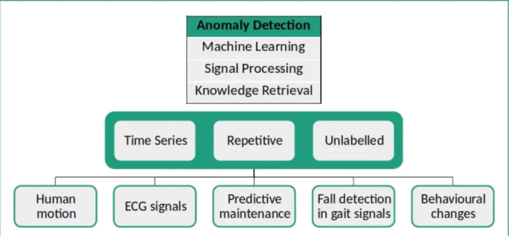
With this solution, it is intended to have a new work study technique that may also be used in various domains, such as human motion, ECG signals, predictive maintenance, fall detection in gait signals and behavioural changes. All this examples have in common the fact that all of them generate quasi-periodic signals in normal circumstances, if cor-rectly measured.
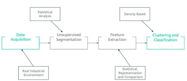
There is a schematic in Figure 1.3 in which there is a brief overview of the techniques required for the proposed solution, the assumption on what data and level of knowledge about that data in which it is supposed to function and various examples of application.
Figure 1.3: Overview of the proposed solution.
This algorithm will then be applied in industrial scenarios to help the prevention of appearance of musculoskeletal diseases and also to assess the training of new employees by giving statistics of their work.
1.5 Summary
1 . 6 . D I S S E R TAT I O N O U T L I N E
Therefore, this dissertation will focus on developing a new algorithm capable of de-tecting anomalies in general data sets combining the aforementioned methods of prepro-cessing and classification. These methods will then be used in a specific manufacturing application in order to be validated in a real world industrial scenario.
1.6 Dissertation Outline
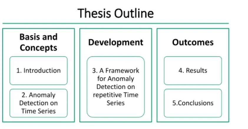
This dissertation is structured as shown in Figure 1.4. The structure is divided in 3 areas: basis and concepts, methods and outcomes.
Thesis Outline
Basis and Concepts
1. Introduction
2. Anomaly Detection on
Time Series
Development
3. A Framework for Anomaly Detection on repetitive Time
Series
Outcomes
4. Results
5.Conclusions
Figure 1.4: Dissertation outline.
C
h
a
p
t
e
r
2
A n o m a ly D e t e c t i o n o n Ti m e S e r i e s
In this chapter, it is intended to provide a better understanding of the concepts that support anomaly detection on time series and also the most widely used methods.
2.1 Time Series
Time series are sets of data points ordered in time. Formally, a time series composed byN data points is represented by
X:={x1, x2, ..., xN} (2.1)
where eachxi,i∈ {1,2, ..., N} corresponds to a data point. These signals let us visualise the behaviour of the underlying process over time. Time series are, thus, important tools to understand real world phenomenons and are used in many applications, such as, meteorological readings, price stock readings, ECG signals, and any data collected by a sensor over time.
In anomaly detection scenarios, a crucial characteristic for the analysis of time series is the periodicity, which is the characteristic of a segment of a time series to repeat itself over time. Mathematically it is represented asX(i) =X(i+T) in whichT is the period of the time series. Hereafter, for simplicity reasons, quasi-periodic time series, which are time series that are repetitive in essence but may have morphology differences in different
"cycles", will be referred to as periodic or cyclic.
2.2 Anomaly on Time Series
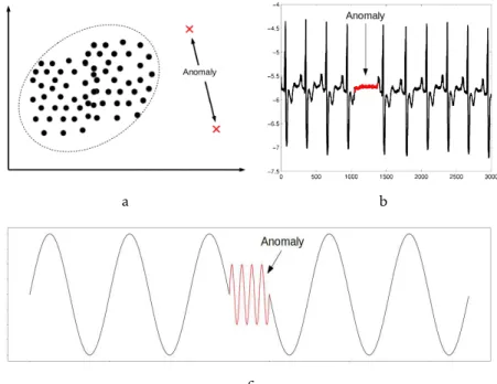
existing anomaly types:
Point Anomaly - An individual point that does not conform well to the whole data set. It is presented an example in Figure 2.1a.
Sequence Anomaly - A sequence of points that does not fit well with the rest of the data set. Example in Figure 2.1b.
Pattern Anomaly - A short segment of data that forms a pattern, but does not conform well to the pattern formed by the rest of the data set. Figure 2.1c shows a simulated pattern anomaly.
a b
c
Figure 2.1: Representation of each anomaly type: a) point anomalies; b) sequence anomaly. Adapted from [1]; c) pattern anomaly.
The main goal of this work is to detect anomalies in periodic time series and, therefore, the principal focus will be finding sequence anomalies and anomalous patterns.
There are various difficulties in the process of anomaly detection and several
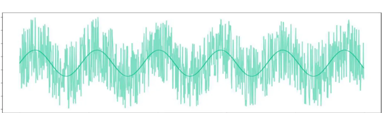
character-istics that have to be taken into account in order to perform accurate anomaly detection. The first problem that must be taken into account, which is present in most data mining settings, is noise. Noise can mask not only the normal behaviour of a time series, but also the anomalous. For example, in Figure 2.2, noise is so relevant that it is almost impossible to perceive the behaviour of the original signal.
The second characteristic to consider is the context. Once anomalies are considered highly context dependent, signals acquired in different domains may have different
con-cepts of anomalies, such as different concepts of normality. Thus, there are points in a
2 . 2 . A N OM A LY O N T I M E S E R I E S
Figure 2.2: Noise influence on a time series. The darker signal can be masked by the existence of noise, represented by the lighter part, making it difficult to find anomalies
or learn the normal behaviour of a time series.
in Portugal, it is normal to find a temperature of 10ºC. However, if this reading is made in the summer, it may be considered anomalous, because it is not usual to have these temperatures by that time of the year. An illustrative example is shown in Figure 2.3.
Figure 2.3: Representation of a contextual anomaly. The temperature is an example of how the context may influence the task of finding anomalies. Here we see that there are other points, such ast1with the same value ast2, yet onlyt2constitute an anomaly. Image
source: [1]
The last characteristic to consider is the frequency of anomalies. There are algorithms that make the assumption that the anomalous sequences or patterns appear less often than the normal data points, however, it might not always be true. For instance, the presence of a worm in computer networks is reflected by a higher amount of anomalous than normal traffic [1].
Moreover, there are various challenges in anomaly detection on time series [15]. The first, is the fact that the portion of the time series that is anomalous is unknown and can be a single point (point anomaly) or a sequence that may correspond to a cycle in a cyclic time series, it may occupy a portion of a cycle or even various consecutive cycles, ultimately reaching the whole time series. Besides, once the morphology of anomalous segments is unknown, it is difficult to select an appropriate distance measure or function
to test different signals of different domains. Furthermore, in multivariate time series, it
the task of anomaly detection in such cases.
Despite the characteristics and challenges that have to be taken into account for anomaly detection, it is possible to formalise the general problem of anomaly detection:
Given a time series X ={x1, x2, ..., xN}, we can segment the time series in M subse-quences as
X={S1, S2, ..., SM} (2.2)
where eachSi, i∈ {1,2, ..., M}is a subsequence ofX composed of a defined number of data points, that may vary from segment to segment. So the time series can be represented as
X ={S1, S2, ..., SM}={{x1, ..., xk1},{xk1+1, ..., xk2}, ...,{xkM−1+1, ..., xkM}} (2.3)
whereki, i∈ {1, ..., M}are the lengths of the corresponding segments,Si, ofX.
The analysis of each subsequence is usually accomplished using a cost function that may, for instance, indicate distance or density. Thus, a subsequenceSiis anomalous if
f unc(Si, Sj)> δ ∀j∈[1 :M] (2.4)
whereSj may correspond to all subsequences exceptSi, a model of a normal pattern, or a set of rules thatSimust obey to be considered a normal segment. The result off unc(Si, Sj) is the anomaly score, which can be considered theanomaly degreeofSi. The definition of the threshold,δ, usually controls the sensitivity of the algorithm.
There are numerous methods used to detect anomalies. In the next sections there will be described the most utilised techniques followed by a brief summary and discussion about them.
2.3 Statistical Methods
This class of techniques is based on one principle: the process that controls the under-lying behaviour of a data set is a stochastic event, thus, it follows a statistical distribution. Thereafter, an anomaly is originated by a different process that does not follow the same
statistical distribution [1]. The key assumption is that normal instances populate high probability regions, while anomalous data is located in low probability regions of the as-sumed stochastic model. These techniques are divided in parametric and non-parametric.
Parametric techniques assume that the normal behaviour of a data set is generated by a parametric statistical distribution. Hence, given an observationx, there is a set of pa-rametersθthat parametrise the probability density functionf(x, θ). The parameters are estimated from the observed data and the anomaly score is the inverse of the probability density functionf(x, θ). Therefore, an observation with higher probability of appearance has an inferior anomaly score than an observation with a lower probability value.
2 . 4 . F O R E CA S T I N G M E T H O D S
The parameters are estimated usingMaximum Likelihood Estimates(MLE) and the anomaly score is often calculated as the difference between the test instance and the parameters,
namely the mean and standard deviation, of the assumed probability density function. There are more relevant statistical tests which can be used in anomaly detection tech-niques and the assumed probability density function can also be changed depending on the application.
Another widely used technique is the Regression Model-Based, in which a regression model is firstly fitted to normal data. Then, for test instances, the residual is used to calculate the anomaly score.
Contrary to parametric techniques, non-parametric techniques do not assume data distribution and use non-parametric statistical models, hence, the model structure is determined by the analysed data. These techniques make fewer assumptions than para-metric techniques. The most basic technique is the Histogram Based, in which the profile of the instances are used to compare them.
The greatest advantage of these techniques is that if the assumed distribution is true, it is possible to justify the classification of each instance and it is possible to make a statistical study of each result, resulting in a robust classification. Otherwise, the greatest disadvantage is that if the assumed distribution does not hold true, the statistical tests are not valid. Furthermore, there are various distributions that may be applied to the same scenario and all of them may be true in some point, which makes it difficult to choose the
appropriate distribution.
2.4 Forecasting Methods
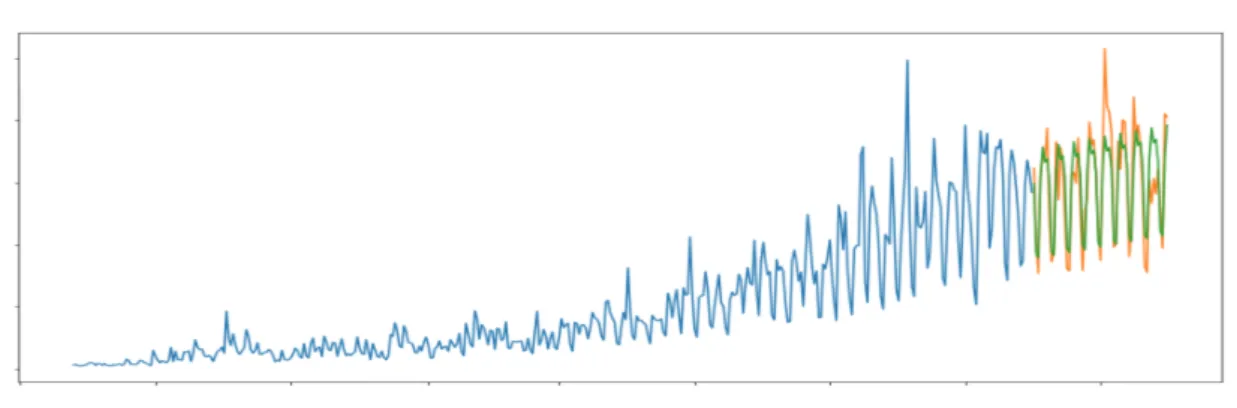
Forecasting methods rely on the apprehension of the normal behaviour of a time series based on its past in order to be able to accurately detect future anomalies. Hence, the first step is to learn the normal behaviour based on the history of the time series and it is critical to choose the correct time-interval to be considered history. This is because, in cyclic events, if the length of the signal that is being learned is inferior to the time of a repetitive unit, the algorithm will not be able to accurately learn the shape of a normal cycle and, thus, it may have a high false hit rate. If the considered history is too long, then the computational complexity can play a role in a way that it might be impossible to analyse the whole data set [15]. In Figure 2.4 there is an example of time series forecasting, in which the blue part is the considered history in order to make the predictions presented in green. The anomaly detection task, which is the second step, consists on the comparison of the predicted model and the true observations, being the anomaly score given by the difference between those. In Figure 2.4, the true observations
correspond to the orange part, that would be compared to the green part if the task was to detect anomalies.
Figure 2.4: Time series forecasting example. The blue part is the history considered to make the predictions, the green part is the achieve prediction and the orange part is the real signal at that time interval for comparison. Image source: [33]
the history parameterm, which is the number of points of the time series to be considered as history and is considered the order of the model, in order to make predictions. There are various models that may be used:
•Moving Average (MA) - MA models represent time series by the application of a linear filter, in which each point is represented by the mean value of the m points sur-rounding it. This means that the time series appears to be smoother. The forecast consists on taking the lastmpoints of the time series and assuming that the next point will have an identical value (it may be considered the addition of noise):
yMA(t+ 1) =µ+ǫt+1+
t−m X
i=0
θt−i·ǫt−i (2.5)
whereθt−i are the model’s coefficients,ǫ
t−i are white noise terms of past observa-tions,ǫt+1is the white noise term of the future observation andµis the mean of the
time series.
•Autoregressive (AR) - AR models represent each series data points as regressions of previous data. The predicted data is the result of the regression of m previous observations and is calculated according to Equation 2.6:
yAR(t+ 1) = t−m X
i=0
βi·y(t−i) +ǫt+1 (2.6)
whereβi is the ith autoregressive coefficient and ǫt+1 is noise at time t+ 1. It is
similar to linear regression, but instead of being only dependent on the current observation, the result is also dependent on previous results.
Autoregressive Moving Average (ARMA) models combine both AR and MA to produce the prediction. It is modelled by Equation 2.7 which is the sum of equations 2.5 and 2.6
yARMA(t+ 1) =µ+ǫt+1+
t−m X
i=0
θt−i·ǫt−i+ t−m X
i=0
2 . 5 . M AC H I N E L E A R N I N G
Another widely known method is the Autoregressive Integrated Moving Average (ARIMA) which works based on the same principle as ARMA, but in the differentiated signal, in
which each data point corresponds to the difference between the actual point and the
previous one.
Non time series based techniques take only into account the information given by the history of themdata points from the recent history of the time series. These techniques, such as Linear Regression and Gaussian Processes would have the form of
y=W·Φ({xt
−m, ..., xt}) +b (2.8)
where{xt−m, ..., xt}are the previousmobservations,W is a weight vector andΦ is a map-ping function (in linear regression,Φ({x
t−m, ..., xt}) ={xt−m, ..., xt}).
The greatest advantage of these techniques is that if the underlying process is contin-uous and dependent on past states, the prediction may be accurate, and so the anomaly detection step is also correct. But if the process is not recursive and the next value does not depend on past values, then the predictions made are inaccurate and anomaly detection becomes impossible.
2.5 Machine Learning
Machine Learning consists of a set of methods capable of automatically detect patterns in data and then use the discovered patterns in decision making scenarios and to predict future data [34]. Ultimately, the goal is always to generalise the learned pattern for any input data, and to do so, there is one assumption that is made: If two pointsx1andx2are
similar, then so should be the corresponding outputsy1andy2.
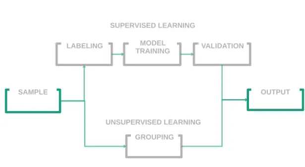
In Figure 2.5 there is a typical pipeline of application of machine learning techniques, in which the top part corresponds to the supervised learning workflow and the bottom part corresponds to the unsupervised learning methodology.
Those workflows are made accordingly to the supervision degree required to learn the referred patterns, that are:
Supervised learning - In this type of learning the goal is to apprehend the behaviour of a dataset given a train set where each data point is labelled and categorised. A set D={(x
i, yi)}Ni=1 wherexi is a data point, yi is its label, Dis called training set and N is the number of training examples, represents a possible representation for a data set used in supervised learning. Likewise, there is a test set which has unlabelled data that can be different from the training set. Given the training set,
SAMPLE
LABELING
SAMPLE
MODEL
TRAINING VALIDATION
GROUPING
SAMPLE OUTPUT
SUPERVISED LEARNING
UNSUPERVISED LEARNING
Figure 2.5: Typical pipeline for machine learning techniques. On top there are the pro-cedures taken by supervised learning techniques and in the bottom is the procedure for unsupervised learning techniques.
of people, images, time series data or sentences. The label or output may also have different designations. It can be considered categorical, if it has a finite number
of possible values yi ∈ {1, ..., C}, in which case, the task is called classification, or it can be a real-valued scalaryi ∈R being then called regression. One variant of this is ordinal regression, consisting of a categorical output that has a natural order, such as any grade system [34]. The most known example of supervised learning classification algorithm is thek-nearest neighbour. Given a labelled dataset and a testing data point, the label attributed to the test point is the most common label among itsknearest neighbours, which are thekclosest points to the test point in the training set.
Semi-supervised learning - In this type of learning the goal is to apprehend the be-haviour of a data set given a train set in which there are labelled and categorised data points and data points that are not labelled [35]. Formally,X is the training set containingN inputs, that containsXs={(xi, yi)}li=1andXu ={xi}Ni=l+1beingXs
2 . 5 . M AC H I N E L E A R N I N G
data is labelled, instead of mixing the nature of the labelled data. This means that the (un)labelled data carries information to answer the questionp(y|x) (what is the probability of the output to bey given that the input isx). If we consider boolean data sets, the process is simple because we could label every data from a class, thus, every sample that does not belong to that class, belongs to the other. In anomaly detection, for example, it is common to have a training data set with the normal in-stances labelled. This is helpful in situations where there are few or none anomalies in the training set. For example, in spacecraft fault detection, an anomaly scenario is not easy to model because it would implicate an accident [35]. The typical ap-proach used in such techniques is to build a model for the class corresponding to normal behaviour, and use the model to identify anomalies in the test data [1]. The opposite case, the training set containing only anomalies is difficult to work with
because anomalous instances may have significantly different morphologies and
they may be unknown for most contexts.
Unsupervised learning - In unsupervised learning the goal is to apprehend the behaviour of a dataset without prior knowledge about it [34]. Thus, all data is unlabelled at the beginning andX={xi}Ni=1is a possible representation of the inputs to unsupervised
learning techniques. The goal is to discover interesting structures that can divide the data instances into clusters of related data, even if that relation is unknown, such that inner cluster variance is minimum and inter cluster variance is maximum. Clustering algorithms may be divided in exclusive or non-exclusive algorithms. In exclusive algorithms each sample is assigned to a specific cluster, while in non-exclusive algorithms, each sample may belong to more than one cluster. Exclusive algorithms include partitioning, hierarchical and density-based algorithms. Parti-tioning, in which it is included, for example, k-means and k-medoids, clustering is performed based on the distance to a specific point, corresponding to the centroid of the cluster. In k-means, that point is the gravity-center of each cluster, while in k-medoids it is the data point closest to the center. Each data point is thus assigned to the cluster with closest centroid or medoid. Hierarchical methods construct a dendogram based on the similarity between samples in order to form clusters. The difference between methods is the way in which the dendogram is constructed
(top-down or bottom-up) or the similarity measure. Density-based algorithms partition data points based on the density of each data point. Points belonging to dense spaces are considered clusters and points sparser in space are considered outliers. Non-exclusive algorithms, such as C-means or Gaussian Mixture Models use the concept of probability and fuzzy analysis in order to group data points. In C-means it is used a fuzzy approach in order to assign a probability of belonging to a given cluster to each data point, which means that it may belong to various clusters with different probabilities. Gaussian Mixture Models assume that each cluster has the
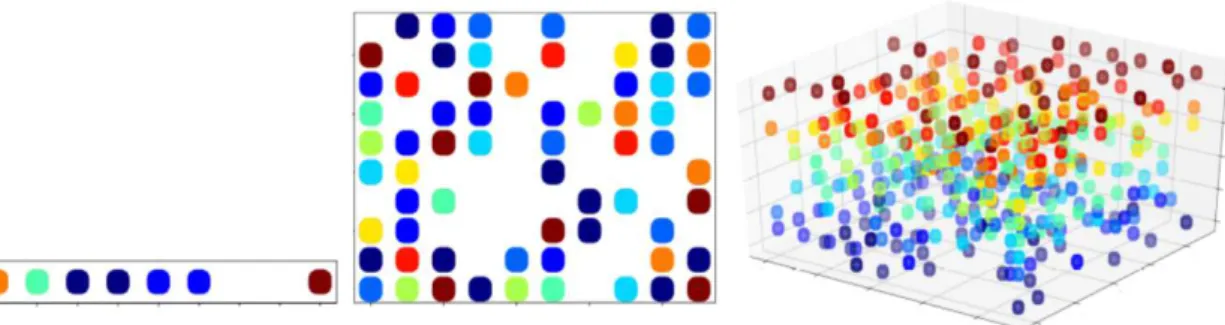
belonging to each cluster based on the spatial location relative to the center of each probability-density function. In Figure 2.6, there is an example of various cluster-ing algorithms applied in various datasets in order to comprehend the difference of
their application.
Figure 2.6: Clustering algorithms exemplified. Adapted from: [36]
Unsupervised learning is more used than supervised, because it does not require manual labour to label any data set, which is a process that might be slow, may be expensive and may hide important information that a human might discard without realising. For example, retailers who track customers purchases use this informa-tion to detect groups of customers with similar interests or similar buying patterns and can then use this for marketing purposes, among other applications [37].
Machine Learning has been used in several applications such as email spam filtering, image classification, prediction of future’s stock market price given current market con-ditions and signal processing [34].
2 . 5 . M AC H I N E L E A R N I N G
tedious, require an expert to do it, and it may be necessary a great amount of labelled data in order to train supervised algorithms. Furthermore, even though unsupervised algorithms, such as, clustering algorithms, do not require labelled data, it is necessary to understand the outcome of those algorithms, which might not be simple.
2.5.1 Time Series Metrics - Features
In machine learning it is usual to represent each sample by specific characteristics, designated as features. This process is usually designated as feature extraction and the task is to extract the most relevant features to characterise the analysed samples. Relevant features are defined as features that allow the distinction of samples in different classes,
namely, the classes that we are trying to assign them to, but are notredundantor irrele-vant. Redundant features are features with high values of correlation, which means that they carry similar information, while irrelevant features are those which are not able to distinguish samples of different classes, usually because the range of values that they take
is narrow. Feature selection is the step in which both irrelevant and redundant features are eliminated and allows the simplification of models, shorter training times, reduced overfitting (thus increased generalisation) and to avoid the curse of dimensionality. The curse of dimensionality arises from increased number of variables, because with that aug-mentation the number of configurations of the data rises exponentially [38]. In Figure 2.7 it is clear that an increase of dimensionality (left to right) leads to more complex solutions, the number of regions of interest increases and the task of generalisation becomes harder because of the specificity of those regions. Thus it is important to select appropriate features depending on the domain of application.
Figure 2.7: Curse of Dimensionality illustrated. In the left image it is easy to distin-guish between different areas of interest, in which each area is represented by a cell. As
the number of dimensions is increased (left to right), the number of regions of interest increases and the generalisation process becomes harder, because each region becomes more specific.
important to scale the features correctly, but that task is not trivial. An extensive research of methods that help to address that problem is given in [39]. In cluster analysis there are three widely known scaling procedures: Z-score standardisation, range standardisation and variance-to-range standardisation.
• Z-score standardisation - each variable is multiplied by the reciprocal of the standard deviation. Hence, each feature is left with unit variance, which means that fea-tures with higher variance are more penalised than feafea-tures with low variance. The formula used for this scaling is presented in Equation 2.9
z(1)ij =xij−x¯j σj
(2.9)
where ¯xj is the mean value of the set andσj is its standard deviation.
• Range standardisation - each variable is multiplied by the reciprocal of the range of the feature. The result is that every feature is left with unit range and if it is centred around zero (zero mean), the resulting range of values is from −0,5 to 0,5. Thus, every feature has equal contribution to the result. The transformation is made by 2.10.
z(2)ij = xij
max(xj)−min(xj)
(2.10)
wheremax(xj) andmin(xj) are the maximum and minimum value of each feature set, respectively. In this case the value of variance can be different for each feature.
• Variance-to-range ratio weighting - this scaling technique takes into account both variance and range information. This type of scaling is appropriate for cluster-ing techniques because it gives a general idea about theclusterabilityof each feature. According to [39], there are three steps to calculate the appropriate value, starting by the calculus of Mj by Equation 2.11.
Mj =
12·V ar(xj) max(xj)−min(xj)
(2.11)
whereMj is an indicator of the clusterability ofxj, increasing with that characteris-tic. Relative clusterability is given by Equation 2.12.
RCj = Mj min(Mj)
(2.12)
A set of features with no clusterability will have RC=1 and the increase of clus-terability leads to an increase of RC. The transformation is made using Equation 2.13.
zj(3)=z(1)j ·
v u u t
RCj·[max(z
(1)
min)−min(z
(1)
min)]2
2 . 5 . M AC H I N E L E A R N I N G
where z(1)j is the matrix of the transformation of the xj variable and z
(1)
min is the transformation corresponding to the value with minimumM value calculated by equation 2.11.
Features scaling can be made prior or after feature selection, and the used method to achieve it is usually chosen empirically by experimentation and analysis of results. The sensitivity towards features extraction and selection represents another disadvantage of machine learning methods, because their selection may have a high influence on the achieved outcome.
2.5.2 Validation
Validation consists on the evaluation of the results achieved in the classification or clustering phase. For that, it is required the definition of various concepts that charac-terise the classification of each sample. First, the expected outcome corresponds to the true class of the classified sample, whereas the predicted class corresponds to the classi-fication given by the model which may be supervised, semi-supervised or unsupervised. In the case of anomaly detection there are two classes: normal and anomalous. Based on these concepts, it is possible to define four quantities to assess the classification:
True Positives (TP) - number of samples classified to the same class as the expected class. In anomaly detection it corresponds to assigning the label of anomalous to an anomalous sample.
False Positives (FP) - number of samples classified to a different class in relation to the
expected class. In anomaly detection it corresponds to label normal samples as anomalous.
True Negatives (TN) - number of samples that do not correspond to the class that is under consideration classified as different from that class. In anomaly detection
scenarios, it corresponds to label normal sample as normal.
False Negative (FN) - number of samples that correspond to the class that is under anal-ysis classified as different from that class. For example, labelling an anomalous
sample as normal.
This quantities are usually expressed in the form of a confusion matrix as shown in Table 2.1.
Table 2.1: Confusion matrix representation.
Expected Label Predicted Label Negative Positive
Negative TN FN
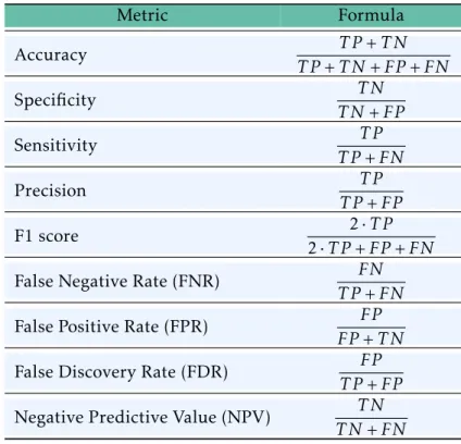
Moreover, it is possible to calculate diverse metrics in order to clearly compare the results achieved by different processes. Those metrics are expressed in Table 2.2.
Table 2.2: Validation metrics.
Metric Formula
Accuracy T P+T N
T P+T N+FP+FN
Specificity T N
T N+FP
Sensitivity T P
T P+FN
Precision T P
T P+FP
F1 score 2·T P
2·T P+FP+FN
False Negative Rate (FNR) FN T P+FN False Positive Rate (FPR) FP
FP+T N False Discovery Rate (FDR) FP
T P+FP Negative Predictive Value (NPV) T N
T N+FN
![Figure 2.6: Clustering algorithms exemplified. Adapted from: [36]](https://thumb-eu.123doks.com/thumbv2/123dok_br/16547364.737005/40.892.233.594.271.764/figure-clustering-algorithms-exemplified-adapted-from.webp)