A look into the 3D world of a cell: how 3D simulations can shed lights on morphogenesis

Universidade de Lisboa

Faculdade de Ciências

Departamento de Informática

A look into the 3D world of a cell: How 3D simulations can shed

lights on morphogenesis

Tiago António Falcão Vermelho Maié

Dissertação

Mestrado em Bioinformática e Biologia Computacional

Biologia Computacional

Universidade de Lisboa

Faculdade de Ciências

Departamento de Informática

A look into the 3D world of a cell: How 3D simulations can shed

lights on morphogenesis

Tiago António Falcão Vermelho Maié

Dissertação

Mestrado em Bioinformática e Biologia Computacional

Biologia Computacional

Orientadores:

Doutora Verônica Grieneisen (JIC)

Doutor Francisco Dionísio (FCUL)

Universidade de Lisboa

Faculdade de Ciências

Departamento de Informática

A look into the 3D world of a cell: How 3D simulations can shed

lights on morphogenesis

Tiago António Falcão Vermelho Maié

Dissertação

Mestrado em Bioinformática e Biologia Computacional

Biologia Computacional

Orientadores:

Doutora Verônica Grieneisen (JIC)

Doutor Francisco Dionísio (FCUL)

Contents

1 Introduction 1

1.1 General introduction to modelling . . . 2

1.2 Cellular Potts Model . . . 7

1.3 Dimensional dilemma . . . 13

1.4 Biological Background . . . 14

1.5 Cell Surface Mechanics . . . 17

2 Materials and Methods 20 2.1 Simulations . . . 20

2.2 3D Layer visualization . . . 22

2.3 2D Enhanced visualization . . . 22

3 Results 25 3.1 Basic simulation environment and patch distribution . . . 25

3.2 Basic cell behaviour in 3D and 2D simulations of a single cell . . . 27

3.3 Effect of non-biological parameters in 3D and 2D simulations . . . 29

3.4 Parameter diversity in 3D simulations . . . 29

3.5 Volume conservation effect on simulated cells . . . 32

4 Discussion 37

Acknowledgements

I would like to express my thanks to:

• Dr. Verônica Grieneisen and Dr. Stan Marée for everything really, accept-ing me in their group, for the support, valuable advice, patience, words of encouragement and confidence on my capacities throughout the realization of this work.

• Prof. Dr. José Feijó, whose advice urged me to accept an academic route which has enhanced my future.

• The whole Grieneisen and Marée groups, for being a welcoming, friendly and supportive group from the day I stepped into the lab/office.

• Yara Sanchez-Corralez and Micol De Ruvo whose friendship and support helped me not miss home as much.

• Mrs. Marian Binks whose help with the bureaucracy from work to housing was simply awesome.

• My wonderful girlfriend, Ana Marques, for the continuous love, support, patience and encouraging words without which this work might not have been completed. Also for her precious insight which helped improve this work.

• My brother, José Maié, partner in crime who is always ready to make someone laugh and whose presence through skype lighted up my lonely room in Norwich.

• My parents for their unconditional loving, financial (and anything else that I can think of) support from my very first day at school.

• The AirRivals community and Gameforge4D staff (mostly, Martina Herdt, Stephanie Susanto, Linus Krämer) for supporting and helping me through-out my gaming career which enabled me to pursue my studies abroad. • The other two CAT team members, James Rogers and Gábor Bartucz, for

the training, support and companionship. Without them I would have never won any competition.

• Gameforge4D and MasangSoft, for allowing me to travel across the world, as well as (inadvertently) funding most of my studies in Norwich.

• Lastly, to all my family and friends, for supporting me in all my decisions, without you none of this would be possible.

Resumo

A célula é a unidade básica da vida. Estudar a biologia e a física por trás do comportamento celular é da maior importância, de forma a obtermos um con-hecimento mais profundo a cerca de qualquer problema biológico. Neste estudo trabalhamos com um modelo (Cellular Potts Model) em 3D de uma célula onde vamos observar algumas das mais básicas propriedades da célula. Para trabal-harmos com um modelo, primeiro precisamos de perceber o que é um modelo, para que serve e quais são as suas limitações. Com isto em mente, um modelo pode ser definido como uma representação ou descrição simplificada de algo com estrutura conhecida. Nesta representação serão aplicados cálculos e predições com o objectivo final de perceber aquilo que estivemos a simplificar. Devido à el-evada complexidade dos sistemas biológicos, a modelação é uma ferramenta fun-damental para nos ajudar a compreender o mundo à nossa volta desde macro a micro sistemas. Ao utilizarmos modelos como ferramentas para testar as nossas hipóteses temos ainda a vantagem dos custos destas experiencias serem mais baixos do que experiencias realizadas in vivo/in vitro, mais rápidas e podemos assumir com um maior grau de confiança quais as variáveis que estão a influ-enciar a nossa experiência. Neste trabalho vamos usar o Cellular Potts Model (CPM) para tentar perceber algumas propriedades celulares relacionadas com a forma da célula e com a adesão desta a outras superfícies. O CPM define a es-trutura de uma célula biológica com base no arranjo ou configuração de um

con-junto de células generalizadas. Cada uma destas células generalizadas é repres-entada numa grelha celular como um domínio de locais na grelha (pixels/voxels) que partilham o mesmo índice (o ID da célula), um conjunto de estados inter-nos e um conjunto de campos auxiliares. Este sistema celular evolui ao alterar aleatoriamente e a cada intervalo de tempo, uma amostra de locais na grelha, transformando-os (ou não) num dos vizinhos que o rodeia (o local vizinho tam-bém é escolhido aleatoriamente). O processo que escolhe estas transformações é guiado pela equação Hamiltoniana, uma equação de energia efectiva. Esta equação é o aspecto fundamental deste modelo e descreve o comportamento e as interacções celulares. É na equação Hamiltoniana que consideramos os ter-mos que guião a adesão celular, uma função que é fundamental e essencial para qualquer tipo de vida complexa existir. É também na equação Hamiltoniana que tomamos em consideração o volume e a conservação de volume celular. A evolução do sistema, explicada muito sucintamente em cima, é guiada pelo al-goritmo de Metropolis. A cada ciclo do alal-goritmo de Metropolis temos aquilo a que chamamos de MCS (ou Monte-Carlo Step) que representa o nosso intervalo de tempo básico. A cada ciclo do algoritmo calculamos a diferença energética na equação Hamiltoniana entre duas conformações celulares, antes do processo de transformação (explicado em cima) e depois do processo de transformação. Finalmente, aceitamos ou não a transformação se esta for favorável à célula se-gundo os princípios de minimização de energia a que o modelo obedece. Um dos aspectos principais deste trabalho foi o de este ter sido desenvolvido num mod-elo a três dimensões. Isto é importante pmod-elo facto de a maior parte do trabalho científico desenvolvido actualmente continuar a ser em duas dimensões. Os ar-gumentos que suportam este acontecimento são o facto de apesar de um estudo ou modelo em 3D nos fornecer mais informação, esta informação pode não ser de grande valor, relevante ou ser demasiado complexa. A explicação em 2D é suficiente para explicar os fenómenos mais interessantes do objecto de estudo e

o esforço computacional para correr uma simulação em 3D é demasiado elevado para valer a pena. No entanto pensamos que deixar uma dimensão inteira de parte num sistema como o de uma célula animal é uma aproximação demasi-ado simples a um sistema onde se sabe que a forma, volume e posição da célula têm uma grande influência no seu comportamento. Para entendermos como o CPM funciona e em que se baseia, temos que perceber o seu background bioló-gico. As células eucarióticas podem em geral ser definidas por três componentes principais, o núcleo, a membrana plasmática e o citoplasma. Neste trabalho focamo-nos em dois destes componentes, a membrana plasmática e o córtex ce-lular, uma camada especializada do citoplasma que se observa na face interior da membrana plasmática. É com estes dois componentes que as moléculas de adesão celular (CAMs) interagem principalmente. As CAMs podem ser dividi-das em dois grandes grupos, as CAMs que controlam interacções célula-célula e as CAMs que controlam interacções célula-matriz extra-celular. O primeiro grupo é maioritariamente composto por proteínas transmembranares da família das caderinas, enquanto o segundo é composto por proteínas transmembranares da família das integrinas. As CAMs interagem principalmente com os filamen-tos de actina presentes no córtex celular, sendo a actina a principal proteína do citoesqueleto que controla a forma e estabilidade da célula, então esta in-teracção é da maior importância para entendermos como a célula se comporta quando adere a algo. No nosso modelo conseguimos de uma forma generaliz-ada, reproduzir o comportamento das CAMs e do córtex celular. Conseguimos também, controlar outros factores como o volume da célula e a dinâmica dos filamentos de actina. A relação que fazemos entre parâmetros biológicos e parâ-metros computacionais têm por base as mecânicas que controlam a superfície celular. Células e tecidos, até um certo nível de abstracção, podem ser descri-tos como tendo um comportamento semelhante ao de bolhas e espumas, sendo que tentam minimizar a sua superfície celular de modo a adquirirem uma

con-figuração energética mínima. Esta minimização é guiada pelo córtex celular, formando uma espécie de tenção superficial celular. Esta tenção superficial (ce-lular), semelhante à que os líquidos apresentam, pode ser usada para inferir e interpretar comportamentos celulares e vice-versa. Neste trabalho, para além das simulações que desenvolvemos, criámos também dois métodos de visualiz-ação que ajudam à leitura e interpretvisualiz-ação dos resultados visuais obtidos pelo modelo. Os dois métodos são aplicados nas simulações em 3D. O primeiro numa representação em 3D da célula a ser simulada e mostra-nos como a célula se vai distribuindo pelo espaço ao longo do tempo. O segundo método - também aplicado em tempo real - mostra-nos uma representação da célula a 2D, nas quais conseguimos ver vários dados sobre a célula. No nosso ambiente de simu-lação somos capazes de criar células com a forma e na posição que pretendemos. Podemos também mudar o substrato, tornando-o heterogéneo, neste contexto, temos substrato normal (com fraca interacção com a célula) e fibronectina (com forte interacção com a célula). Tal como com a célula, podemos alterar a forma e posição dos diferentes tipos de substrato assim como a sua força de interacção com as células. Neste ambiente de simulação somos capazes de representar célu-las com diferentes características, assim tentamos comparar as célucélu-las que con-seguimos criar no nosso sistema com outras previamente descritas num estudo numa representação a 2D do CPM. Durante este processo, descobrimos que, ao contrário do que estava descrito no estudo, as experiências com as quais estáva-mos a tentar comparar resultados não representavam a célula de uma forma biologicamente viável. Procurámos então outros parâmetros que mostrassem diferentes comportamentos celulares e que ao mesmo tempo fossem biologica-mente viáveis. Esperamos com este trabalho despertar a curiosidade do leitor para o campo da modelação em 3D no âmbito da biologia celular. Para além disto, introduzimos novos métodos de visualização enquadrados no CPM e finalmente discutimos e comparamos dados com investigação feita previamente.

Abstract

We live in a 3D world, yet we are taught most of the classical biology in 2D. Our vision of biological cells, is often taken from histological cuts or 2D confocal slices. This has led to biophysical models of the cell to often being made in only two dimensions as well. In this work I use and adapted a computational biophys-ical tool, the Cellular Potts Model, into 3D. I used it to recreate a cell spreading on a protein lattice to which it can adhere to a bigger or a lesser extent. This very controlled experiment is often used as a paradigm to probe essential bio-physical properties of cells. Tuning several cellular parameters, like adhesion, membrane tension and internal osmotic pressure, I investigated to what extent a minimal description of biophysical properties could capture steady state cell behaviour and developed visualization tools so that a better understanding could be provided through the model. Importantly, I was able to compare and contrast my findings to previous interdisciplinary efforts performed in 2D. This shed light on basic properties of the Cell Surface Mechanics, and generated predictions re-garding the biological experiments. Finally, we suggest how new experiments should be performed that could report 3D-dependent behaviour (which would pass unnoticeable in 2D).

Chapter 1

Introduction

“As our circle of knowledge expands, so does the circumference of darkness surrounding it.”

– Albert Einstein.

Cells are the basic unit of life. Studying the biology and physics behind cell behaviour is of the utmost importance in order to have a deeper understanding of (mostly) any other biological problem.

Here we will work with the 3D model of a cell. We will study some of the prop-erties of the most basic unit of life, with a quantifiable and reproducible method using the Cellular Potts Model (CPM) to accomplish this. The CPM is a model that has been thoroughly tested and has shown results on several different oc-casions [5, 4, 21, 13, 25].

Cell shape is of the highest importance in morphogenesis [11], we are focused in understanding the mechanics involved between cell adhesion and cell shape and how these can be better understood from a 3D point of view rather than the common 2D approach.

1.1

General introduction to modelling

According to the Oxford Dictionary, the word “model” had its origin in the late 16th century and it was denoted as a “set of plans of a building”, nowadays however, this is the meaning of “model”:

Noun

1. a three-dimensional representation of a person or thing or of a proposed structure, typically on a smaller scale than the original;

2. a thing used as an example to follow or imitate;

3. a simplified description, especially a mathematical one, of a system or pro-cess, to assist calculations and predictions;

4. (. . . )

Although it has even more definitions, we don’t need to go any further. A model can therefore be, a simplified representation and description of something, with a known overall structure, to assist calculations, predictions and to, ultimately, understand the original “something”. A realistic approach to modelling is to admit that a model is simply a means to understand certain characteristics or aspects of the system1. A model will always have its flaws and we don’t actually want to recreate the whole reality but just have a minimal representation of it. Since we know the flaws and shortcomings of our model, we know to which questions it may answer and perhaps even more importantly, to which it may not. We then ask ourselves if this minimal representation is sufficient to explain

the phenomenon at hand or if more complexity needs to be added (For a really interesting and similar analogy read [20]).

A model recreating reality would be trivial to do if the initial system was that of a ball rolling down a hill, or an apple falling of a tree, but as we go to more and more complex systems, a fluid going through a pipe/cavern network, a planetary system, or even something that we’ve produced ourselves, for example, the com-puter in which I’m typing right now. If one tries to model or rather, understand any of these examples as a whole, we will get confused with the overwhelming amount of information to process, categorize and ultimately understand. This is because the complexity of the system (e.g. a laptop, the human eye, a migrating cell) is so high that we need to break the problem into little pieces in order to understand it better. Then piece by piece, we might, produce the exact copy of our original system with a full understanding of everything that is happening with and within it.

Compare now a physical system with a biological one. Although both systems obey to the same physical laws, the biological system will usually be much more complex. Not necessarily because the system is more difficult to understand but because the amount of understanding that we have on the subject is considerably smaller. Biological systems have high amounts of redundancy, living beings in general need to be robust, as do their own systems and the systems they live in. Adding do the redundancy, even a simple bacterial cell found in the wild, has several systems in itself that we simply don’t know how they interact with each other. Furthermore we might not even, with current technology, be able to know it at all since when we try to fix and observe these cells in vitro, they don’t behave the same way, the same molecules are not produced and secreted, the environment is not the same, the surrounding bacterial flora is not the same. Physical systems are therefore in this sense, easier to understand and predict. A

circuit board with a given set of connections, will always transport information in the same predictable way if the initial condition stays constant. Tomorrows weather forecast will be predicted, by a model, with a high amount of confidence because even though the weather as a whole is a highly complicated system, all it’s parameters and rules are fairly well understood and so the model is able to capture the major features and behaviours of the target system, the weather, at least on the near-future.

On a possible future in which we know how every single molecule of a cell in-teracts with each other, in which we have the activity profile of every enzymatic molecule well defined, in which we know how the cell responds to every single environmental cue, on this utopic future where we know everything, then pre-dicting the behaviour, shape or any other cell action or trait should be fairly easy to achieve.

As explained above biological systems have, in general, an overwhelming com-plexity. Consider the following system and all the interactions in between its levels, in this planet we have a biosphere, composed of different ecosystems, oc-cupied by different communities, composed of different populations in which we have a variable number of organisms, if we consider this organism to be an an-imal for example, then, each organism is composed by several different organ systems, these organs are made of different tissues, these tissue are organized masses of cells, these cells are composed of different intracellular organs, made of molecules, made of atoms. The previous sentence, abnormally large, sheds light on the problem exposed earlier. As Alan Turing put it in his 1952 paper “One cannot at present hope to make any progress with the understanding of such systems except in very simplified cases” [26], which is just as true now as it was then. The complexity is so overwhelming that trying to come up with an explanation or description for even an extremely simple animal like C. elegans,

is extremely troubling.

This is where modelling excels. As a modeller you initially come up with a rel-atively small set of rules and parameters to explain a given phenomenon. Then you try to disprove it by testing your model. If it doesn’t explain your phe-nomenon, you change and adapt your rules, you give it new parameters, if it eventually explains your phenomenon, that’s good. It’s not actual proof that the explanation for the phenomenon is still the right one but it’s probably a step in the right direction. Further testing and comparisons with the actual phe-nomenon will eventually lead to a complete or partial explanation. It also helps to communicate your findings to fellow scientists or even specialists from other areas since the model itself is defined quantitatively with equations, paramet-ers and some given variables instead of qualitatively like much of biology is still taught [10].

A good model would be one that fully explains the features of the system and can be used to make prediction using as little information as possible. However at times, it is impossible, to know if the model being used is a good representation of reality because a model can only be as good as the knowledge we have about the subject. Hence what can be considered a good model today, may not be so tomorrow, either because we discovered that the mechanics, implemented in the model, don’t actually work that way in reality, or because another model is able to explain the same phenomenon with more fidelity (possibly in a more simplistic way).

There are countless examples that show us exactly how modelling helped us understand a bit more about our complex world. Here in particular we are trying to understand biological systems. A few landmark studies in this area are the works of Hans Meinhardt and Alan Turing (the very same mathematician best known for his cryptology and artificial intelligence studies) on morphogenesis

(more specifically, biological pattern formation) [16, 26].

Furthermore performing in vivo or in vitro experiments is always a hassle. First we can’t always ensure that we are only experimenting with one variable, then it’s highly time consuming and usually really costly. Experimenting in silico might be time consuming initially, building and understanding the model and simulations but after that stage it’s pretty straight forward, inexpensive and we can, to a certain degree, be sure which variables are at play.

As a young scientist with a classical biology background, with experience work-ing on plant, animal and unicellular organisms, if I were to do a quick thought exercise on how many possible errors that I (or my colleagues) have done unwill-ingly or unknowunwill-ingly, I believe it could easily reach the thousands mark. This is because, for every experiment, there are a great number of factors that might contribute for the overall outcome of our experiment that we just don’t know or care about, for example, systematic and random errors. A recent research has shown that exposure of mice and rats to male but not female experimenters induced a robust physiological stress response that results in pain inhibition which can affect the apparent baseline responses in behavioural testing [23]. Such results might put years of research in jeopardy. Adding to this, an easy and frustrating example, when working with plants or bacteria, it is incredibly easy to find our cultures contaminated (even when following all the procedures to avoid such problems), redoing all the work takes time and money, especially if the plants have a long life cycle or the bacteria strains we were working with are not easy to obtain.

Change is good and I believe that the change that we will mostly observe going forward, is the approach of modelling as a whole to the mainstream biological sciences.

1.2

Cellular Potts Model

In this work, I will use a modelling formalism, the Cellular Potts Model, to try and understand some of the properties that a cell has while adhering to a sub-strate to which it has more or less affinity. I will discuss some of the relevant details concerning the cells’ shape later on, but for now, the interesting research question here is the fact that the cell shape can influence how the cell chooses its own future or lineage, how basic biophysical properties can change such com-mitment and how we can use such properties to influence the cells comcom-mitment ourselves.

With the role of a model and modelling in general being understood, I will now explore the methods and background of the modelling framework that is going to be used in this thesis since it is essential to its understanding.

The Cellular Potts Model (CPM from hereafter) [7, 5], was created in the early 90’s by François Graner and James Glazier. The model is an extension of the large-Q Potts Model which itself is an extension of the Ising Model.

The Ising Model is an early and simple ferro-magnetism model which is usually represented on a lattice where at each site we have the atomic spins, able to interact with its neighbours via an energy function. The Ising Model was used to explain the continuous phase transition that occurs on ferromagnetic materials below their corresponding Tc2. In ferromagnetic materials, stable small regions called magnetic domains3 form without the aid of an external magnetic field, thus yielding a net magnetic polarization [4].

There are several steps in between the model extensions but these magnetic

2_{The Curie temperature T}

cis the temperature where a material’s permanent magnetism,

fer-romagnetic behaviour (below Tc) changes to induced magnetism, paramagnetic behaviour (above

Tc)

Table 1.1: CPM notation. Lattice site (vector of

integers) Cell with index of − → i Type of cell σ(−→i ) − → i σ(−→i ) τ (σ(−→i ))

domains are going to be the future cells of the CPM. The most important ad-aptations made to transform the Ising model into what the CPM is today were volume conservation and the introduction of cell types with different properties [4].

The CPM was created with the intent to model and explain cell sorting which it accomplished to great success [7, 5].

The CPM defines a biological cell structure consisting on the configuration of a set of generalized cells, each represented on a cell lattice as a domain of lattice sites (pixels/voxels) sharing the same cell index (the cell’s ID), a set of internal cell states for each cell (Table 1.1 on page 8, Figure 1.1 on page 9) and a set of auxiliary fields [4].

Basically, this cell system dynamically evolves by changing a random sample of these lattice sites (pixels or voxels) at each time-step. These sites will transform into one of their randomly chosen neighbours or stay as they are, which repres-ents a cell extension or a cell retraction. Whether this transformation occurs is calculated by the Hamiltonian, the effective energy function.

H_CPM = X − → i ,−→j neighbor J (τ (σ(−→i )), τ (σ(−→j ))) · (1 − δ(σ(−→i ), σ(−→j ))) + λ(V0− VT)2 (1.1)

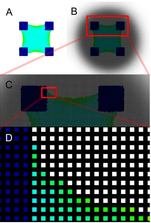
Figure 1.1: Basic representation of how the lattice would look on a 2D envir-onment. A - Basic 2D cell representation on our model; B, C, D - Casting and zooming in on a grid so that we can observe each lattice site.

and interactions. Even though our Hamiltonian looks like equation (1.1), many other terms can be added to represent constraints and other phenomena. Regarding the CPM Hamiltonian, its most important term describes cell adhe-sion, be it to other cells or to the environment, cell adhesion is necessary for any form of complex life to exist. Cell adhesion, biologically speaking, will be discussed in Section 1.4. In the CPM, adhesion is defined as a boundary energy

X − → i ,−→j neighbor J (τ (σ(−→i )), τ (σ(−→j ))) · (1 − δ(σ(−→i ), σ(−→j ))) (1.2)

that depends on J (τ (σ(−→i )), τ (σ(−→j ))), the boundary energy per unit area between two cells (σ(−→i ), σ(−→j )) of a given type (τ (σ(−→i )), τ (σ(−→j ))) at the interface between two neighbouring pixels/voxels, where the sum is for all neighbouring pairs of lattice sites −→i and −→j , where the neighbourhood range might be greater than one4 _{(and usually is, to avoid anisotropic grid-effects). Also note that J-values} (boundary-energy coefficients) are symmetric,

J (τ (σ(−→i )), τ (σ(−→j ))) = J (τ (σ(−→j )), τ (σ(−→i ))). (1.3)

The Kronecker delta term (1 − δ(σ(−→i ), σ(−→j ))) is there to ensure that lattice sites of the same generalized cell do not count towards our calculations, since if σ(−→i ) = σ(−→j ) then δ(σ(−→i ), σ(−→j )) = 1 and (1 − δ(σ(−→i ), σ(−→j ))) = 0. Otherwise, if σ(−→i ) 6= σ(−→j ) then δ(σ(−→i ), σ(−→j )) = 0 and so (1 − δ(σ(−→i ), σ(−→j ))) = 1.

Volume conservation, represented as λ(V0− VT)2 is the only constraint that we implement in this version of our model. Here, V0 represents the cells, current volume, how many voxels it has, while VT represents the cells target volume. Finally λ represents the cells membrane inelasticity. A smaller value of λmeans

that the cell membrane will be quite elastic, allowing it to stretch so it can tol-erate greater deviations from the cell’s target volume, while greater values of λ mean that the cell membrane will be inelastic and so it won’t deviate much from the cells target volume. Note that if the inelasticity term is 0, then the cell in question won’t have any volume conservation, allowing it to disappear or to grow infinitely depending on the interaction values with the surrounding environment.

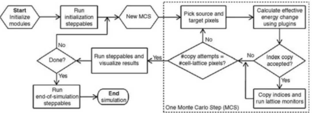
The evolution of the model is actually driven by what is called the Metropolis algorithm. This algorithm, using the CPM Hamiltonian, is structured as follows:

1. Randomly select a lattice site. This site will be called the target site−→i of the generalized cell σ(−→i )

2. Randomly select a neighbouring site of the target site. This will be called the source site−→j of the generalized cell σ(−→j )

(a) If the source site−→j belongs to the same generalized cell as the target site−→i ,σ(−→i ) = σ(−→j ), then nothing else happens and we jump back to 1.

3. With the effective energy function, the Hamiltonian, calculate the current configuration energy (Hinitial), also calculate the configuration energy if the target site was changed to the source site (Hf inal), that is, if σ(

− →

i ) → σ(−→j ) 4. Calculate the difference this change would do to the total effective energy

5. Decide whether this change will be accepted with a Boltzmann probability: p(∆H) = p(σ(−→i ) → σ(−→j )) =        1 if ∆H < 0 e(−∆HT ) if ∆H ≥ 0 (1.5) 6. Go to step 1

Steps 1 through 5 are called a index-copy attempt and in a lattice with N sites, a time-step, or rather a Monte-Carlo step (MCS from hereafter) is defined as N index-copy attempts.

The main elements of the CPM is thus, the Hamiltonian - the effective energy function - and the dynamics, which are about evaluating and accepting unfa-vourable changes. It’s on the Hamiltonian that we are going to compute many of the important aspects of the model such as cell adhesion, volume conservation and membrane fluctuations, as energy terms. We can also compute, for example, chemotaxis and persistency as force terms, although these are not applied dir-ectly on the hamiltonian but rather during the metropolis algorithm when we are calculating the variation of the total energy, the dynamics. For chemotaxis, this is made through a modification of equation (1.4) into

∆H = Hf inal− Hinitial− µ(ctarget− ctrial) (1.6)

where c represents a possible chemoattractant concentration value at both sites, the one copying (“source”) and the one being copied into (“target”) and µ is the strength of this chemoattractant.

It is with the Hamiltonian that we are going to compare how our system is evolving comparing the present energy configuration of a site with a possible future energy configuration of the same site given its neighbours.

Figure 1.2: Basic representation of how the software of a CPM model works. Figure from [25].

1.3

Dimensional dilemma

Most CPM studies are made in a two-dimensional (2D) simulation environment. The argument supporting the preference for 2D over three-dimensions (3D) is that although 3D might provide us with more information, this information might not be valuable, relevant enough or it’s just too complex. The 2D explana-tion is sufficient to explain most interesting phenomena [17] and finally that the computational effort needed to run a 3D simulation is too heavy [6]. Different types of models do lead with dimensions in different ways, finite-element mod-els (FEM) and segment-based modmod-els do require great qualitative extensions to generalize in 3D. Furthermore research is usually done in 2D because scientists consider cells quasi-2D (the height being negligible), or - in the case of epithelial tissue - they consider the tight junctions as restraining the cells 3D shape into a thin 2D problem. 2D simulations are great in their own way, they are faster and easier to generalize. Also, pedagogically, biology has traditionally been taught in 2D since the main object used to teach this subject is the book, hence when we see a 2D simulation running, it is usually easier to conceptualize what is hap-pening. Traditional microscopy further enforces the 2D concept since only until very recently we started to be able to consistently have high quality 3D images

of tissues.

However we believe that by leaving a whole dimension aside in a system, for example, a generic animal cell, where we know that shape, position and volume have a great influence in its behaviour, is ultimately a naive approach that we can now start to distance/deviate ourselves from.

It has been shown, for example, that in regards to cell sorting, parameter de-pendencies established in 2D cannot be extrapolated to 3D as these overstate and oversimplify some features of the cell like the role of active cytoskeletal fluctuations and the role of heterotypic interfaces [8].

More so, nowadays with the technological advancements made in the last 20 years, the computational time and effort needed to run a 3D simulation is much smaller. Hence in this thesis we are going to explore, in a 3D environment, how a generalized animal cell, given certain parameters, spreads on a flat heterogen-eous substrate with different adhesive properties. We will focus on finding out which cell shapes and forms, as a result of basic biophysical considerations, are stable and which are not.

1.4

Biological Background

Eucaryotic cells can, in general, be narrowed to three main components which include everything else, the nucleus, the plasma membrane and the cytoplasm. In this work we are particularly concerned with two of these components, the plasma membrane and the cell’s cortex, a specialized layer of cytoplasm on the inner face of the plasma membrane.

The plasma membrane is the cells’ border with the rest of the world (e.g. cells from the same or different types, extra-cellular matrix, medium, substratum,

soluble and insoluble molecules), therefore it is the first physical structure of interaction that the cell has with the outside environment. There’s a panoply of molecules responsible for these interactions but those we are interested in are the cell adhesion molecules (CAMs). CAMs can be divided in two big groups, the CAMs that control cell-cell adhesion and the ones that control cell-matrix adhe-sion. The former is mainly composed by the Cadherin family of transmembrane proteins, the latter is mainly composed by the Integrin family of transmembrane proteins. Both of these have the ability to communicate with the cytoskeleton and vice-versa. Without these, complex life forms would not exist.

Cadherines function as transmembrane proteins that indirectly link the actin cytoskeletons of the cells they join together. This interaction is essential for effi-cient cell-cell adhesion, as cadherines that lack their cytoplasmic domain cannot hold cells strongly together [1].

Integrins also function as transmembrane linkers but between the cytoskeleton and the ECM. Like the cadherines, most integrins are also connected to bundles of actin filaments (also called F-actin). A cell can regulate the adhesive activ-ity of its integrins from within. Integrins also function as signal transducers, activating various intracellular signalling pathways when activated by matrix binding. Integrins and conventional signalling receptors often cooperate to pro-mote cell growth, cell survival, and cell proliferation [2].

The cell’s cortex is where a great majority of the actin filaments are located. The cytoplasm of eucaryotic cells is spatially organized by a network of protein fil-aments known as the cytoskeleton. Actin filfil-aments determine the shape of the cell’s surface and are one of the three main protein filaments of the cytoskeleton (the other two being microtubules and intermediate filaments). These flexible and dynamic filaments form several types of cell-surface projections and are ne-cessary for whole-cell locomotion [1]. Myosin also has a role in determining the

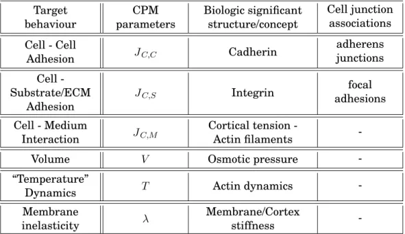
Table 1.2: CPM - Biology Summary. Target behaviour CPM parameters Biologic significant structure/concept Cell junction associations Cell - Cell Adhesion JC,C Cadherin adherens junctions Cell -Substrate/ECM Adhesion JC,S Integrin focal adhesions Cell - Medium Interaction JC,M Cortical tension -Actin filaments

-Volume V Osmotic pressure

-“Temperature”

Dynamics T Actin dynamics

-Membrane

inelasticity λ

Membrane/Cortex

stiffness

-cell’s shape. Myosin can render an actin network more fluid through its motor activity in vitro and can remodel actin filaments in vivo [11], however it can also make it contract [12]. Filaments in the cell cortex are the main responsible for the cell’s cortical tension, which can be defined as the cell’s apparent surface tension due to the contractile microfilaments of the cortex and their interaction with the membrane [11].

Maintenance of the cell’s shape and stability is thus mainly provided by a close relationship between CAMs and actin filaments. A brief and comprehensive summary of the relation between the CPM model and the biological background is provided on Table 1.2 on page 16.

1.5

Cell Surface Mechanics

In this thesis we will work with a generic animal cell. The behaviour of such cells is restricted to a set number of processes such as cell division, apoptosis, cell growth, cell migration and cell-shape changes. Particularly, we will study the interaction between the cell and the extracellular matrix (ECM). Cells adhere to the ECM through different cell surface receptors, CAMs, the major class of these are integrins like previously discussed. Interacting with the ECM enables the cell to sense mechanical cues, such as forces, from the ECM and react accord-ingly, this process is known as mechanotransduction [28]. For example, in the case of mesenchymal stem cells (MSCs), a change in the cell shape, from spread and flattened to round can account for the activation of one differentiation path and consequent phenotype, osteoblastic, instead of another, adipogenic, respect-ively [15].

Here however, we only wish to consider the passive biophysical elements that shape a biologically living cell, so we will only focus on the membrane, its sur-face, and the forces exerted on the membrane by the cells cortex and the pos-sible mechanics surrounding them. This base-line level of understanding, when contrasted to other active processes, allows the biologist to evaluate what is gen-erated through active cytoskeleton remodelling, and what would be expected by homogeneous interactions alone. Therefore, we wish to evaluate to what extent a simple cell shape behaviour can be explained by this limited set of biophysical properties. Using as an inspiration biological experiments, biophysical paramet-ers in the simulation can be changed leading to differential outputs. These can be compared to the observed biological cells, or can lead to further predictions. Up to a certain level of abstraction, cells in a tissue can be described in a similar framework as the behaviour of bubbles and froth (surface minimizing cellular

elements); likewise, embryonic tissues can present similar properties to immis-cible fluids, such as cell sorting and tissue rounding [24]. It is also known that single cells behave similarly to bubbles or liquid droplets, often spherical in or-der to minimize their surface area and tissues present foam-like behaviours. With this in mind, we will here mostly consider the factor that controls to a large extent the cells equilibrium shape, the (cell) surface tension [11].

In order to make this assumption a few concepts and notions on cell surface mechanics need to be established.

The differential adhesion hypothesis (DAH) proposed by [24], suggests that dif-ferences in inter-cellular adhesion guide tissue segregation, mutual envelop-ment and the sorting of embryonic tissues. This hypothesis, which has been confirmed experimentally5 [3], lies on the assumption that the homophilic as-sociation of cadherins is distinct from the heterophilic asas-sociations. It states that cells can, over time, explore several configurations and arrive at the lowest-energy configuration. Computer simulations, namely with the CPM, had the utmost importance in supporting the significance of the DAH in cell sorting [5]. However the DAH by itself cannot explain cell sorting at a biologic level, that is, if only the DAH is taken into account, the rate at which cells sort does not hap-pen at a biologically sustainable rate. For this to haphap-pen, chemotaxis, haptotaxis and pressure gradients need to be taken into account [13].

Surface tension can be defined as the free-energy change when the surface of a medium is increased by a unit area and it is usually expressed as J oules · m−2_. Increasing the surface area of an oil droplet in water requires an energy δe, which is proportional to the area increment δs, such that δe = σ × δs, in which σ is the surface tension of the liquid.

5_{Research shows that the aggregate surface tensions are a direct, linear function of cadherin}

The reason a liquid droplet or a bubble naturally assume a spherical shape, is because with this shape, it has the minimum surface area for its given volume, therefore the surface energy will also be at its minimum. In comparison, the cell’s surface area tends to be minimized by the cortical tension, which is an important ingredient of cell surface tension and the shape of isolated cells [11]. I will use cell shape as a manner to re-interpret the parameters that are driving it.

As discussed in 1.4, CAMs and the cell cortex maintain a close relationship in order to ensure the cell’s stability and define its shape. However, the shape itself also provides feedback on the cell stability [14]. With this in mind, in this work we will utilize the cell shape to re-interpret the parameters driving it. That is, even though we have well defined parameters that can be used to define how the cell is going to behave (see 1.2), if we take the cell shape alone, we can also infer and interpret which kind of parameters are at play.

Chapter 2

Materials and Methods

2.1

Simulations

The 3D simulation environments can be described as a 3-D cuboid lattice consist-ing of 200 voxels/ pixels/ units wide, 200 voxels/pixel/units long and 100 voxels/ pixel/ units tall, with a single cell nucleating from the centre of the bottom face of the cuboid environment. This face represents the substrate. The substrate is composed of a neutral material which doesn’t interact (strongly) with the cell, and patches of a material that do interact strongly (alike fibronectin patches) with the cell. The patches are all of the same size, all disposed at the same dis-tance from each other and are purposely centred on the substrate as to avoid a simulation bias. The cell, unless started randomly, is also centred as to avoid any bias. However, if we wish, the cell and the patches can be started with different conformations.

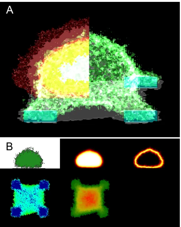
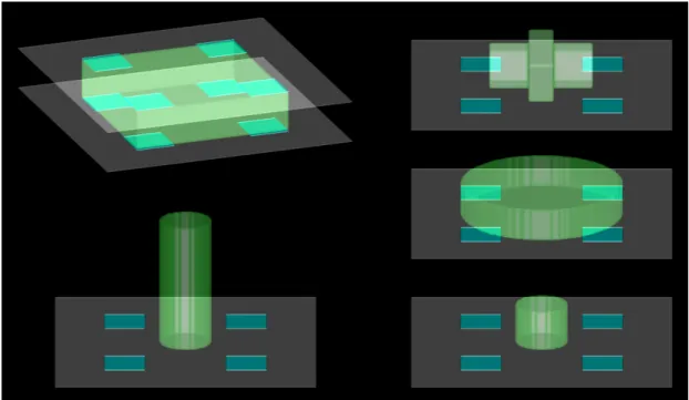
Figure 2.1: Example of the visual output of our model. See Figure 2.2 on page 23 and Figure 2.3 on page 24 for an explanation of how to read panel A and B respectively.

2.2

3D Layer visualization

With the objective of being able to extract more information from 3D images of the cell, we created a novel method of visualization that basically divides the cell into different layers according to how often a voxel, belonging to a cell, occupies that position over time. This method, similar to a 3D heat map, eases visualization and conceptualization of what is happening during the simulations and enables us to observe the space occupancy of the cell while the model is running (Figure 2.2 on page 23). This information tells us where the cell is over time, and how flexible or stiff certain membrane interfaces are.

2.3

2D Enhanced visualization

The 2D Enhanced visualization that is created when the 3D simulation runs has several different views (Figure 2.3 on page 24). This visualization runs live while the 3D visualization is also visible, enabling us to observe live intuitive statistics of the cell while the model is running.

F igure 2.2: 3D visual output and vi sualization tool -Here we show a few examples of how the 3D simulation environment looks and how the visualization tool appears if only one la yer w as active at a time . V oxel occupation is set from the moment we activate the method until the present time , hence for practical reasons , ha ving the method active since t = 0 might not be the best idea since if the cell shrinks from t = 0 to t = 100, then the dark red la yer will clutter most of the visual output. As with any vi sual element of the simulation, we can set it’ s viewing state from opaque , to transparent, to invisible , allowing us to observe any element of the simulation in specific if so is des ired . The discrete la yers shown in this image are just a comprehensive w a y to show them, we usually run the simulations with all the la yers on top of eac h other . W e can also define where in the cell the visualization tool will be run.

F igure 2.3: 2D visual output and visualization tool -Here we show an exampl e of the 2D visual output of our 3D simulation. T o ea ch of the 5 panels represented there’ s a correspondent colour bar at the bottom right of the image . On the top row we ha ve 3 panels with a cross-section of the cell. Here we usually ha ve a vertical cros s-section of the cell. W e can define where this cr oss-section happens . On the bottom row we ha ve 2 panels showing a top-down view of the cell. Note that the panel number 2 on the first row of the image is highly related in terms of information pr ovided to our 3D visualization tool. As suc h, these two methods are activated at the same time (MCS).

Chapter 3

Results

3.1

Basic simulation environment and patch

distri-bution

2D and 3D simulations are run. When 3D simulations are run, a 2D live over-view of the simulation is also created2.1. These are ran for a period of time set by us (after a set number of MCS the simulation stops). Cells are coded as interact-ive cells, like the biological cell, or a special kind of cell that it’s not interactinteract-ive, like the medium, the substrate and the fibronectin patches. All the cells are initiated with a given shape, in a given position, with a given set of parameters. Initial shape and position can sometimes be randomized or specifically tailored by us 3.1.

Patches of fibronectin can be created with different shapes, at different positions, with different number of replicates and with different spacing between them. We often use fixed sized squares with a regular pattern throughout the simulation environment.

Figure 3.1: Example of several environmental starting conditions in our simu-lation environment. We can change the initial size and shape of the cell. We can also change the size, shape and position of the substrate and fibronectin patches as shown in the the first example.

Data like the volume, area and height of the cell and positions with which the cell is connecting with the substrate are obtained.

Note that even though we here show the whole simulation environment, during our simulation the whole environment is not shown due to how computational demanding that would be (we would have to render the whole environment in-stead of just the region where the cell is).

3.2

Basic cell behaviour in 3D and 2D simulations of

a single cell

The first simulations ran were with the objective to show the behaviour of a simulated cell would be close to that of a living cell in terms of shape. Every other simulation ran is a modification of this first experiment. A parameter study was performed and a window of acceptable parameters was found. We focused mainly on studying the interaction energies (J-values), temperature and the membrane inelasticity variables.

Our 3D simulations are an extension of the 2D simulations with a new spe-cial type of cell (the medium) and another dimension given to the simulated cell, height. The 3D simulations also have built in additional visualization tools that ease the process of comparing the 3D simulations with the 2D simulations (Figure 2.3 on page 24). Comparisons between 2D and 3D models can be done not only by comparing the information given by visualization tools and the 2D simulations but also by comparing data like area occupied by the cells on the substrate (for 2D and 3D) and area vs volume (2D vs 3D).

F igure 3.2: Standard starting condition of our experiments . Cells are initialized with 124 voxel width, 124 voxel depth and 31 voxel height. P atc hes are created in the substrate and ha ve 31 voxel width, 31 voxel depth and a spacing of 62 voxels between eac h other . Initialized like this , cells ha ve an initial volume of 476, 656 voxels and an init ial area of 15,376 “pixels”.

3.3

Effect of non-biological parameters in 3D and 2D

simulations

As a proof of concept, simulations with parameters that are not biologically feas-ible were also performed. These examples (Figure 3.3 on page 30) mainly show us what would happen if volume conservation didn’t exist in our model. In these experiments we also tried to show simulations where an interesting behaviour was shown by the model.

3.4

Parameter diversity in 3D simulations

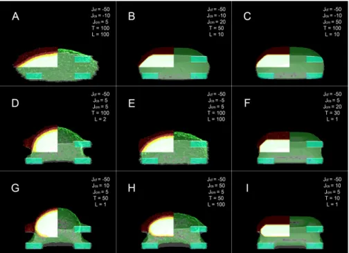
Even though a wide parameter study had already been established, within the window of acceptable parameters, there were still many possible configurations. Here we show a resumed compilation of the different behaviours obtained from this exploration. All pictures were taken at 3333 MCS. It’s interesting to observe how some of these behaviours would be completely missed if we were observing the same cells in 2D from a top view. Panels D, G and H (3.4) are particularly remarkable as these would basically appear as a cell with the same shape if were observing it from a 2D top view even though they are extremely different. Cell H has a great penalty for interacting with the substrate (Jcsis fairly high) hence it barely interacts with it. Meanwhile cell D even though it appears to have nearly the same shape, since the interacting energy between itself and the substrate is not too high, it shows plenty of interactions with the substrate as shown by the pixel occupancy.

F igure 3.3: Proof of Concept -no volume conservation. A -Cell with biologically acceptable parameters; B -Cell with parameters equal to that of A, except for the membrane inelasticity (volume conservation) parameter whic h w as set to 0; C -Cell with parameters equal to that of B , except for the interaction energies between the cell and the substrate whic h w as changed from 10 to -10; D -F -Cells with different interaction energies . Interaction energies (J-values): Jcf = cell-fibronectin; Jcs = cell substrate; Jcm = cell-medium. T = temperature . L = λ = membrane inelasticity (volume conservation).

Figure 3.4: Compilation of a small set of different cell behaviours we can re-produce in our model. Interaction energies (J-values): J_cf = cell-fibronectin; Jcs = cell substrate; Jcm = cell-medium. T =temperature. L = λ =membrane inelasticity (volume conservation).

3.5

Volume conservation effect on simulated cells

Several simulations were run to test the effect that the volume conservation (area conservation in 2D) parameter λ has on the simulated cells. In this exper-ience we considered 3 different patch conformations while varying neighbour-hood assumed by the model and the volume conservation parameter λ (Figure 3.5 on page 33 and Figure 3.6 on page 34).

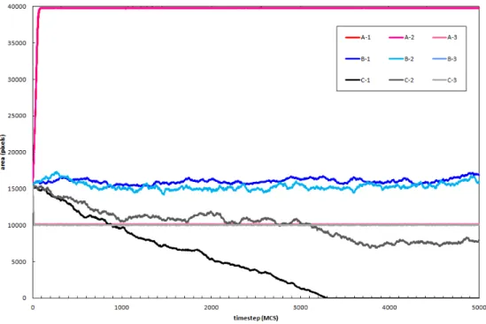
Extremely interesting results were obtained. First we show that in 2D a cell with an extremely small λ behaves as if volume conservation didn’t exist as it can be seen in A-1 and C-1. In A-1 (and A-2) the cell area increases as much as possible covering the whole fibronectin filled substrate and substrate and far surpassing the target area (A₀ = 104). On the other hand, in C-1, since the cell doesn’t have any highly favourable surface interacting with it, it does what a body whose behaviour is driven by energy minimization would do, it gets smal-ler and smalsmal-ler until it disappears. Also as expected the cell that has λ = 1 maintains its target volume along the simulation be it over a fibronectin sub-strate or over a bare subsub-strate. B-3 in particular is also interesting, the cell leaves a little “island of cell” behind and goes to a more stable energy minim-izing shape adhering to 3 fibronectin islands instead of the usual 4. A counter intuitive result however is C-2, where λ is really low and so it should behave like C-1. However, since the neighbourhood range assumed by the model in that case is low, it is hard for the model to resolve a metastable minima. Still, we expect that the cell would disappear if given enough time.

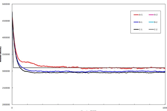
We also ran the same type of experience on our 3D model with interesting res-ults (Figure 3.7 on page 36). Firstly we see that all the simulations that have λ = 1 (experience A,B,C-2) have a really sharp approach to the target volume (V₀= 310000). This is due to two things, first the value of λ (in this case, volume

F igure 3.5: Area conservation. Experiences represented here are grouped by letters and numbers where the same letter denotes the same patc h conformation while the same number denotes the same cell parameters . Pictures of the simulations are shown between 1 and 5000 MCS at different intervals . Lett ers: A -patc h occu pies all of the substrate; B -four square patc hes (side size of 31 px and spacing between them of 62 px) of equal size occupy the substrate; C -there is no patc h present in the substrate . Numbers: 1 -λ = 0 .0002 , T = 250 (following [27]) and neighbourhood assumed of 6; 2 -λ = 0 .0002 , T = 250 (following [27]) and neighbour hood assumed of 1; 3 -λ = 1 .0 , T = 250 and neighb ourhood assumed of 6. On all simulations the cells are started on the same spot with the same size .

Figure 3.6: Area conservation graphic. Areas shown correspond to the cells in 3.5 and follow the same notation.

conservation), is fairly high (in comparison to what is used in experience 1), second, there’s a great difference between the volume with which the cell is ini-tialized (Vi = 476656) and the cell’s target volume (V0 = 310000). It is therefore highly favourable for the cell to decrease its volume.

Nevertheless we can see that unlike the 2D experiment where the cells with a low volume conservation either increased unrealistically (scenario A), main-tained a somewhat stable volume (scenario B) or unrealistically decreased until disappearing (scenario C), in the 3D experiment all the cells suffer a decrease in volume, this is due to the fact that here the cells also interact with the medium, since the interaction with the medium is not favourable, the cells minimize the interaction with it.

Looking now at the results from experience 1 from Figure 3.7 on page 36, these were not fully expected but can still be understood. A-1 behaved as expected,

the cell spread through the whole fibronectin substrate and once this happened since the contact with the fibronectin patch is highly favourable, it maintained its volume over time. B-1 and C-1 did not behave as expected though. These two experiments show a (volume) behaviour that follows a tangential line over time. I was expecting C-1 (like the behaviour of C-1 in Figure 3.6 on page 34) to disappear. Further experiments (results not shown) show that even though the volume conservation parameter is really small, in our 3D model, it still contrib-utes to enough to the model for the cell to maintain a V ≈ 290000. Effectively having λ = 0 does show a behaviour similar to that of C-1 in Figure 3.6 on page 34, as it can be seen in panel B of Figure 3.3 on page 30.

Figure 3.7: Volume conservation graphic. Experiences represented here are grouped by letters and numbers where the same letter denotes the same patch conformation while the same number denotes the same cell parameters. Here we plot between 1 and 1000 MCS but the simulation was ran until 5000 MCS, however all the data follow a linear trend as it can be seen from around 500 MCS. Letters: A - patch occupies all of the substrate; B - four square patches (side size of 31 px and spacing between them of 62 px) of equal size occupy the substrate; C - there is no patch present in the substrate. Numbers: 1 - λ = 0.0002, T = 250, Jcf = −250, Jcs = 10, Jcm= 5; 2 - λ = 1.0, T = 250, Jcf = −250, Jcs = 10, Jcm= 5. On all simulations the cells are started on the same area with the same volume.

Chapter 4

Discussion

This work allowed us to (1) create a straightforward working platform where we can observe how a 3D cell would behave on an heterogeneous substrate and where we can change, tinker and adapt many of its aspects, (2) shed light on the differences observed when running a 2D and a 3D simulations with great visu-alization tools and which implications these differences have, (3) better analyse, compare and contrast my findings with previous 2D CPM studies and (4) predict how a real cell would behave based on the behaviour observed in our model. The model we have developed is a great working platform to study cell shape. It’s a highly customizable tool which allows a researcher interested in cell shape, cell adhesion and cell surface mechanics to study, analyse and test several hypo-thesis before ever having the need to do lab work. This coupled with the great visualization tools that we have developed allow the research to better learn how the cell in the model behaves and more importantly which conclusions can be drawn from the simulations.

We believe that these tools, although not entirely new, are a great way for stu-dents and researchers new to the 3D cell modelling subject to learn more deeply

about the issue.

Now, regarding our results related to volume and area conservation. In [27] ex-plained how a cell that spreads on a protein lattice adopts an energy minimizing shape. Here we are introduced to a 2D CPM residing on a square lattice, repres-enting cells which are homogeneous and whose cytoskeleton and nucleus are not explicitly taken into account. The authors characterize their CPM Hamiltonian as

H = Jcs· Aa+ Jcm· pcell+ λA(Acell− A0)2 (4.1) and their Boltzmann probability distribution as

p(∆H) =        1 if ∆H < 0 e(−∆HT ) if ∆H > 0 (4.2)

The authors then build, based on the Hamiltonian, two adimensional paramet-ers, M (equation (4.3)) and S (equation (4.4)), that reflect independent features of the CPM. Parameter M represents a measure of the competition between the elastic compressibility of the cell body and the stress fibres contractility, while parameter S represents a measure of the competition between the interface fluc-tuations and the stress fibres contractility.

M = λA· A 3_/2 0 Jcm (4.3) S = T Jcm· A 1_/2 0 (4.4)

An increase in M leads to a more contracted cell, while an increase in S leads to a higher amplitude of fluctuations at the cell membrane.

Finally the authors compute several values for M and S for a given cell con-formation, a squared cell covering four adhesive spots, eventually reaching an

agreement as to what these values should be for living cells, M = 20 ± 5 and S = 0.25 ± 0.3. The objective of the authors with this study is to find the meta-stable minima of an adhesion energy landscape. In other words, for a given cell with certain biophysical properties, which is the best suited shape on an adhes-ive landscape.

As our initial objective was to generalize this to 3D, and compare and con-trast results, we sought to understand and recreate their findings. Surprisingly enough, when replicating the experiment, we discovered that the value of λ (the area elastic compression modulus) the authors were using was so low (∼ 0), it practically didn’t have any contribution to the Hamiltonian, effectively having λ = 0 did yield the same results.

What this means is that if a cell with these given parameters was initialized over an area without any patches of fibronectin, the cell (in the simulation) would disappear in a few time-steps (Figure 3.5 on page 33). This is because, without a volume constraint, or a really small one, and the fact that the CPM (and all of Cell Surface Mechanics Models) favours energy minimization, noth-ing stops the cell from decreasnoth-ing its volume (and its energy), until it disappears. Furthermore if the cell was effectively initialized, already spread over the 4 ad-hesive spots, but with the ability to reach any other fibronectin patches, then nothing would stop this cell from infinitely increasing its area as long as there were fibronectin patches in reach. This is because the J value corresponding to the interaction between the cell and the fibronectin patches (J_cf) was given an unrealistically high negative value (−250), which highly favours this contact. We hereby conclude that this is an unrealistic scenario to represent a living cell as it would (1) not be able to exist in isolation and, (2) supposing it did survive until reaching a surface, when on a fibronectin surface, would then spread out indefinitely and stop being a cell. In fact, the only situation under which the

sim-ulated cell would maintain a cell-like resemblance, would be under the specific and artificial condition of being on a non-adhesive substrate which has located and few, well-placed, adhesive patches. These non-universal parameters, which only yield a “functional” cell in very precise and narrow conditions, should thus be concluded non-relevant to understanding cell surface mechanics.

Furthermore we also discovered that the adimensional parameters chosen, carry little to no information in the cases where they themselves, M and S, stay equal but the underlying variables change. That is, they are overdetermined. The outcome of several simulations where M and S are fixed but their variables are not, practically produces the same results. The authors themselves do it with a set of parameters. Once again setting M = 20 and S = 0.25, we can for example have Jcs = 10 (cell - substrate interaction), λ = 2 × 10−4, T = 250 and A0 = 104 or Jcs = 5, λ = 1 × 10−4, T = 125 and A0 = 104. A simulation run with these parameters is expected to generate essentially the same output , since what we are doing is simply multiplying the Hamiltonian and the temperature by a positive constant. Moreover, these parameters only apply to a 2D in silico situ-ation, and not an experimental cell (which lives in 3D). This could be observed from our study: when we adapted the published parameters to our 3D model (while maintaining the same underlying variables) and ran the simulations, we verified that such overlapping of outputs/results did not occur. That is, fixing M and S while the underlying variables change does not produce the same res-ults. This is because in a 3D model we need to take into account not only the interactions between the cell and the substrate (J_cs) (while M and S are fixed) but also the interactions between the cell and the medium (J_cm) which are not considered in a 2D model. Hence, if we only change the interaction energies of one, the other will still give the same contribution to the Hamiltonian, which will then lead to a different outcome. Which leads us to the next point, that M and S are essentially capturing a scaling property of the system. When we are

picking the values of these parameters, what we are doing is simply multiplying the Hamiltonian and the Temperature by the same positive constant. If all the Hamiltonian terms and the T are multiplied by a positive constant , then the dynamics will be identical, as stated in [4]. This is due to the kinetics in the modified Metropolis algorithm depending only on the sign of ∆H and the ratio value of ∆H/T (see equation 1.5 or equation 4.2).

Our initial goal was to compare our 3D data with that of [27] under similar biophysical settings, with the intention of finding qualitatively and quantitat-ively different results between the 2D and the 3D cases. We hypothesized that such a tight comparison would shed light on how and why cell-shape behaviour is influenced by dimensionality, context, and biophysical parameters. However given the fact that the parameters used in [27] are not in agreement with our experiment design philosophy (the cell would be stable only if a whole given con-formation and patch layout was set), we set our objective to explore 2D and 3D cell shapes ourselves in a non-pre-described manner, searching for instances in which different 3D shapes could result in the same “2D shape” prediction. An important constraint for us was that the qualitatively divergent cell shapes that we explored should always be possible in vivo/in vitro, whilst at the same time we were searching the parameter space for biologically relevant parameters that we hadn’t previously thought of.

Having performed several simulations exploring the parameter space, we found interesting shapes that would have passed undetected in a 2D environment (Fig-ure 3.4 on page 31 and Fig(Fig-ure 3.3 on page 30). An issue with the 2D simulations is how one consider cells interaction with its environment. Should the 2D-model consider the interaction energies only at the boundary of the cell or should it somehow describe the actual medium that exists around the cell, and not just a perimeter-substrate interface? However, even if one opts to include such

inter-actions, how would you represent this medium and substrate along with their interaction energies on a 2D plane at the same time? There does not exist a straightforward solution and assumptions will have to be made.

Modelling in 3D, although at first more challenging from a computational point of view, actually waives the need of such assumptions, and allows us to draw a more direct mapping between the biophysical parameters of the model, and an actual cell. Furthermore it’s impossible to represent complex shapes in 2D. These 3D highly complex shapes are known to have a high importance in cell behaviour and morphogenesis [22, 9]. Even fairly simple 2D shapes, from a top down view, like a square, can actually be represented in a multitude of ways in 3D.

Although were we present great tools, there are still many things can that be improved on our model. Polarity and persistency are not yet implemented. Per-sistency should be a fairly easy addition to make to our model, however polarity brings up important questions. How would one represent cell polarity in a 3D model? Should we implement polarity solely restricted to the membrane? Or should we represent represent the polarity molecules in the cytosol? Or maybe an interchangeable molecule that jumps in and out of the membrane when it’s active/inactive? Despite our implementation process, how would we then visu-alize the process itself? It’s an interesting issue and needs to be delved upon. Further changes that should also be interesting to implement in the model are dynamic patches or a dynamic and mobile substrate as a whole. This would allow us to study cell shape even further by allowing changes to a substrate to which the cell is already adapted to (like in a real environment).

As a whole, the study of cell shape still requires much more investigation as comparatively we still know much more about the 2D geometry of a cell than

Bibliography

[1] B. Alberts, A. Johnson, and J. L. et al. Molecular Biology of the Cell, chapter The Self-Assembly and Dynamic Structure of Cytoskeletal Filaments. New York: Garland Science, 4th edition edition, 2002. Available from: http://www.ncbi.nlm.nih.gov/books/NBK26862/. [2] B. Alberts, A. Johnson, and J. L. et al. Molecular Biology of the Cell, chapter

In-tegrins. New York: Garland Science, 4th edition edition, 2002. Available from: http://www.ncbi.nlm.nih.gov/books/NBK26867/.

[3] R. A. Foty and M. S. Steinberg. The differential adhesion hypothesis: a direct evaluation. Developmental Biology, 278(1):255 – 263, 2005.

[4] J. A. Glazier, A. Balter, and N. J. Poplawski. Magnetization to morphogenesis: A brief his-tory of the glazier-graner-hogeweg model. In A. Anderson, M. Chaplain, and K. Rejniak, editors, Single-Cell-Based Models in Biology and Medicine, Mathematics and Biosciences in Interaction, pages 79–106. Birkhäuser Basel, 2007.

[5] J. A. Glazier and F. Graner. Simulation of the differential adhesion driven rearrangement of biological cells. Phys. Rev. E, 47:2128–2154, Mar 1993.

[6] J. A. Glazier and D. Weaire. The kinetics of cellular patterns. Journal of Physics: Condensed Matter, 4(8):1867, 1992.

[7] F. Graner and J. A. Glazier. Simulation of biological cell sorting using a two-dimensional extended potts model. Phys. Rev. Lett., 69:2013–2016, Sep 1992.

[8] M. S. Hutson, G. W. Brodland, J. Yang, and D. Viens. Cell sorting in three dimensions: Topology, fluctuations, and fluidlike instabilities. Phys. Rev. Lett., 101:148105, Oct 2008. [9] O. Lancaster, M. Le Berre, A. Dimitracopoulos, D. Bonazzi, E. Zlotek-Zlotkiewicz, R. Picone,

T. Duke, M. Piel, and B. Baum. Mitotic rounding alters cell geometry to ensure efficient bipolar spindle formation. Developmental Cell, 25(3):270 – 283, 2013.