Ambiente Água - An Interdisciplinary Journal of Applied Science

(1)

www.ambi-agua.net E-mail: ambi.agua@gmail.com

This is an Open Access article distributed under the terms of the Creative Commons Attribution License, which permits unrestricted use, distribution, and reproduction in any medium, provided the original work is properly cited.

Importance of adequate appropriation of physiographic

information for concentration times determination

ARTICLES doi:10.4136/ambi-agua.2184

Received: 19 Sep. 2017; Accepted: 18 Apr. 2018

Joseline Corrêa Souza; José Antonio Tosta dos Reis*_;

Antonio Sergio Ferreira Mendonça

Universidade Federal do Espírito Santo (UFES), Vitória, ES, Brasil Departamento de Engenharia Ambiental. E-mail: joseline.correa@gmail.com,

jatreis@gmail.com, anserfm@terra.com.br *Corresponding author

ABSTRACT

Concentration time is an important parameter for drainage systems design and is closely related to the physiographic characteristics of a given hydrographic basin. Information from cartographic bases or images obtained by remote sensing, which present certain scales/resolutions, are often employed for the appropriation of concentration times. The present study sought to investigate the influence that the combination of different physiographic information, in different scales, and different calculation methods can produce in concentration times’ values. The applied methodology included a concentration times appropriation methods survey, identification of methods compatible with the study area characteristics, physiographic variables appropriation from information plans at different scales and concentration times determination for different regions. The results show that there is an equivalence between Tulsa District and US Corps of Engineers methods, and that these methods produce higher concentration times estimates than those produced by the George Ribeiro method. For the study area, the maximum calculated relative error was 52%.

Keywords: concentration time, drainage, hydrology, scale, watershed.

Importância de adequada apropriação de informações fisiográficas

para definição de tempos de concentração

RESUMO

(2)

Rev. Ambient. Água vol. 13 n. 4, e2184 - Taubaté 2018

e determinação dos tempos de concentração para as diferentes regiões hidrográficas da área de estudo. Os resultados obtidos mostram que existe equivalência entre os métodos Tulsa District

e US Corps of Engineers, e que esses métodos produzem tempos de concentração superiores

aos produzidos pelo método de George Ribeiro, produzindo erro relativo com valor máximo de aproximadamente 52%.

Palavras-chave: bacia hidrográfica, drenagem, escala, hidrologia, tempo de concentração.

1. INTRODUCTION

Hydrological models are mathematical water systems behavior representations. Among hydrological models, there are the so-called “rainfall-runoff,” which represent rainfall transformation processes and consequent flow propagation in a watershed (Fan and Collischonn, 2014).

The rainfall-runoff models are usually used for flow-data series complementation, hydrograph determination for engineering design, flood forecasting and basin land-use assessment (Ferraz et al., 1999). Shuster and Pappas (2010), Halwatura and Najim (2013), Silva et al. (2014), Walsh et al. (2014), Vinagre et al. (2015) and Cabral et al. (2017) illustrate different possible rainfall-runoff models’ applications.

The concentration time parameter is necessary for determination of peak flow rates and hydrographs formatting by using rainfall-runoff models (Silveira, 2005; Farias Júnior and Botelho, 2011). Silveira (2005), however, observes that the determination of concentration times is a difficult task due to limited information about the applicability of some of the available empirical formulas.

Concentration times estimation can be done by two approaches: the direct, which uses hydrometeorological records or tracers; and the indirect, which uses previously established mathematical expressions for certain regions. Direct methods are widely utilized when hydrometeorological records with discretization intervals shorter than the concentration time or tracer data collected in field surveys are available (Farias Júnior and Botelho, 2011). In Brazil, however, the availability of information is scarce, especially for medium and small hydrographic basins. Therefore, for this type of regions, the alternative that is usually used for concentration time appropriation is the use of indirect methods.

Mata-Lima et al. (2007) divide the indirect methods formulations’ characteristics into two groups: empirical and semi-empirical. According to the authors, the empirical formulations result from correlations and statistical treatment of physiographic variables observed in the field without considering the effect of changes in soil use and occupation, and generally do not require detailed input data. Semi-empirical formulations result from a similar process; however, they also consider the effects of changes in the land use and occupation dynamics and other variables that change over time.

For appropriation of physiographic variables considered in concentration time equations, the use of Geographic Information System (GIS) as a support tool is recurrent. Through GIS it is possible to manipulate digital information plans, available in different scales and resolutions, from which the physiographic variables can be obtained.

(3)

the original scale.

The present study evaluated the influence of physiographic records scale in hydrographic basins’ concentrations time determination. The study area is a medium-sized river basin located in the southwest portion of Espírito Santo state.

2. STUDY AREA

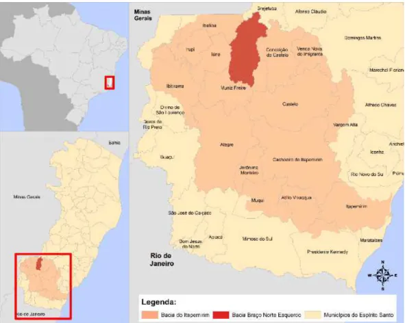
The study area consists of a medium-sized hydrographic basin, called Norte Braço Esquerdo River watershed, which presents an area of 333.52 km² and a perimeter of 111.71 km and is located in the southwest portion of Espírito Santo state (Caparaó region), Brazil, as can be observed in Figure 1. The watershed has as its main water course the Norte Braço Esquerdo River, an Itapemirim River tributary.

The region presents dry temperate climate, with an average annual rainfall of 1,371 mm, and relief ranging from strongly corrugated to hilly. The predominant soils are classified as Red Latosol and Dystrophic Yellow Latosol, degraded by extensive pastures, degraded crops abandonment, coffee plantations and new annual crops implementation, as well as roads construction and maintenance by using inadequate technologies (INCAPER, 2011).

The basin limits were obtained from the set of Level 5 Ottobacias, available in the Espírito Santo State Geospatial Bases Integrated System (GEOBASES).

Figure 1. Braço Norte Esquerdo River basin location.

(4)

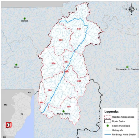
Figure 2. Braço Norte Esquerdo River basin subdivision.

3. METHODOLOGY

Two basic assumptions were established for implementing the used methodology different stages:

• Adoption of low-cost and easily reproduced methodologies, prioritizing the use of free computational tools whenever possible; and

• Use of public domain information, free of charge, provided by public institutions.

3.1. Databases selection

Physiographic characteristics, which represent the basin’s physical characteristics, such as relief, drainage network, vegetation cover, soil and surface use and occupation, among others, are usually extracted from maps, aerial photographs and satellite images. It was decided to use data from digital cartographic bases. In this way, digital files containing information plans in raster or vector format (shapefile format) were manipulated through the Geographic Information System.

In this work, information plans related to relief, drainage network and land use and occupation were used to estimate concentration times. Information plans with dubious origin or low detail level (very small scales) were previously discarded and the other files were submitted to attributes consistency analysis and geometric features representation. This analysis involved information conferencing, file comparison, correction of topological faults and projection systems and coordinates transformations, aiming to work with the data in the same coordinate system and Datum (SIRGAS 2000).

(5)

Table 1. Data sources of physiographic information.

Subject Geospatial data Data type Spatial resolution/scale Source

Relief

Digital Elevation

Model Matrix 90 meters

Empresa Brasileira de Pesquisa Agropecuária

(EMBRAPA) Digital Elevation

Model Matrix 30 meters ASTER GEDEM

Level Curves Vector 1:50,000 GEOBASES

Drainage

network Drainage sections

Vector 1:50,000 GEOBASES

Vector 1:250,000 _{Geografia e Estatística (IBGE)}Instituto Brasileiro de

Use and occupation

Land use

(2008-2010) Vector 1:10,000

Instituto Estadual de Meio Ambiente e Recursos Hídricos

do Espírito Santo (IEMA)

3.2. Concentration times appropriation methods selection

Existing hydrographic basins’ concentration times appropriation methods identification was conducted through a current literature review.

For appropriation methods selection, all methods restrictions were compared with the study area type of occupation, area, slope and talveg length. In this selection stage, three possible outcomes were established:

• Applicable: when all hydrographic basins presented area, slope, talveg length and occupation type within the applicability range established by the concentration time determination method;

• Not applicable: when at least one of the hydrographic basins presented area, slope, talveg length and occupation type outside the applicability range established by concentration time determination method;

• Unidentified restriction: when there was no restriction on the use of the method identified

in the revised literature.

4. RESULTS AND DISCUSSION

4.1. Physiographic information

The equations selected for estimating concentration times involve four variables: a) basin occupation type, b) basin area, c) slope, and d) talveg length. In the subsequent items the cited variables estimated values are presented, considering the different digital cartographic bases used.

4.1.1. Basin Occupation Type

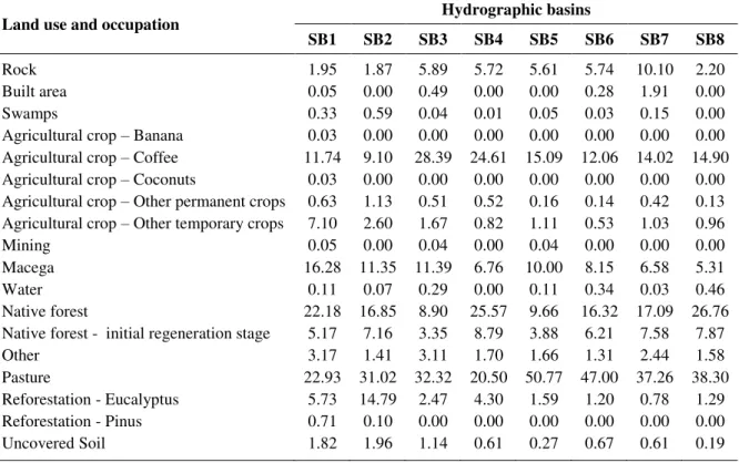
Basin occupation type consists of information related to basin predominant land use and occupation, urban or rural. In order to determine the hydrographic basins’ occupation types, the areas corresponding to each use class were surveyed by using land use and occupation information plans provided by IEMA in the 1: 10,000 scale. Table 2 was produced from this survey, which presents the percentages of areas associated with different types of land use and occupation.

(6)

Table 2. Percentage of area occupied by different land uses and occupation.

Land use and occupation Hydrographic basins

SB1 SB2 SB3 SB4 SB5 SB6 SB7 SB8

Rock 1.95 1.87 5.89 5.72 5.61 5.74 10.10 2.20

Built area 0.05 0.00 0.49 0.00 0.00 0.28 1.91 0.00

Swamps 0.33 0.59 0.04 0.01 0.05 0.03 0.15 0.00

Agricultural crop – Banana 0.03 0.00 0.00 0.00 0.00 0.00 0.00 0.00 Agricultural crop – Coffee 11.74 9.10 28.39 24.61 15.09 12.06 14.02 14.90 Agricultural crop – Coconuts 0.03 0.00 0.00 0.00 0.00 0.00 0.00 0.00 Agricultural crop – Other permanent crops 0.63 1.13 0.51 0.52 0.16 0.14 0.42 0.13 Agricultural crop – Other temporary crops 7.10 2.60 1.67 0.82 1.11 0.53 1.03 0.96

Mining 0.05 0.00 0.04 0.00 0.04 0.00 0.00 0.00

Macega 16.28 11.35 11.39 6.76 10.00 8.15 6.58 5.31

Water 0.11 0.07 0.29 0.00 0.11 0.34 0.03 0.46

Native forest 22.18 16.85 8.90 25.57 9.66 16.32 17.09 26.76 Native forest - initial regeneration stage 5.17 7.16 3.35 8.79 3.88 6.21 7.58 7.87

Other 3.17 1.41 3.11 1.70 1.66 1.31 2.44 1.58

Pasture 22.93 31.02 32.32 20.50 50.77 47.00 37.26 38.30 Reforestation - Eucalyptus 5.73 14.79 2.47 4.30 1.59 1.20 0.78 1.29 Reforestation - Pinus 0.71 0.10 0.00 0.00 0.00 0.00 0.00 0.00 Uncovered Soil 1.82 1.96 1.14 0.61 0.27 0.67 0.61 0.19

4.1.2. Basin Area

The hydrographic basins areas were appropriated from the file containing the Level 6 Ottobacias watersheds limits, adopted for study area subdivision, as mentioned in the item "Study Area". From GIS files software manipulation, the regions areas were obtained by adopting Mercator Transversal Universal Projection System and SIRGAS Datum 2000. The areas values that resulted from the performed process are available in Table 3.

Table 3. Hydrographic regions’ areas. Hydrographic basin Area (km²)

SB1 82.33

SB2 39.70

SB3 32.94

SB4 40.34

SB5 27.33

SB6 57.82

SB7 35.28

SB8 17.77

4.1.3. Talveg Length

(7)

Table 4. Main talvegs hydrographic basins lengths.

Hydrographic

region Main Talveg

Talveg length (km) Error

1:50.000 1:250.000 Absolute _(km) Relative _(%)

SB1 Braço Norte Esquerdo River 21.64 20.55 1.0982 5.07 SB2 Estrondo Creek e do Mata-Pau _{Creek stretch} 13.36 13.12 0.2426 1.82

SB3 Sossego and Braço Norte _{Esquerdo stretch} 10.768 10.68 0.0752 0.70

SB4 Piaçu Creek or Cantagalo and _{Tombos Creek stretch} 10.46 10.26 0.1944 1.86

SB5 São João Creek and Córrego _{Rico Creek stretch} 11.33 11.38 0.0456 0.40

SB6 Mata do Barão Creek and Braço _{Norte Esquerdo stretch} 17.93 17.85 0.0747 0.42

SB7 Ribeirão Vargem Grande Águas Claras Creek and

stretch 13.49 12.06 1.4378 10.66

SB8 Seio de Abraão Creek and Trecho do Braço Norte Esquerdo stretch

10.07 9.91 0.1630 1.62

4.1.4. Declivity

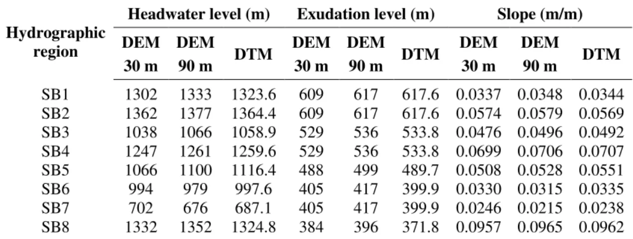
Slope is a variable used in the application of different concentration time determination methods. Since most methods that present restrictions related to slope values employ the talveg mean slope to estimate concentration times, it was decided to use the talveg slope value as the standard criterion for formulas applicability analysis. In this context, the points coordinates corresponding to the headwater and outlet of the main watercourses of each sub-basin were taken into account, considering the drainage network layout available on the 1: 50,000 and 1: 250,000 scales information plans. Then, each main talveg head and outlet points altimetric dimensions were obtained, considering the different sources of information related to the relief. From the obtained altimetric dimensions, each of the main talvegs slope values was determined. The obtained dimensions and corresponding slope values are presented in Tables 5 (scale 1: 50,000) and 6 (scale 1: 250,000).

It is relevant to observe that the talveg slope is a physiographic characteristic that depends on two main factors: a) the drainage network or hydrography, which establishes the trajectory of the water courses and serves as basis for appropriating the talveg lengths; and b) the relief information, which provides information on altimetry. In this work, the information regarding the drainage network presents two different scales (1: 50,000 and 1: 250,000), and the information concerning the altimetric dimensions came from three different sources (level curves, 30-meter resolution DEM and 90-meter resolution DEM). In this way, each hydrographic basin presented six different possible slope values for the main talvegs.

4.2. Concentration times estimation methods

Indirect methods for concentration times determination were identified from a review of the literature. These methods were summarized by McCuen et al. (1984), Paiva and Paiva (2001), Pruski et al. (2004), DNIT (Brasil, 2005), Silveira (2005), Santos et al. (2009), Farias Junior and Botelho (2011), Grecco et al. (2012), Dhami and Pandey (2013) and Porto et al. (2014). The authors present, when available, information regarding each selected method’s

(8)

slope and talveg length - which determine concentration times appropriation indirect methods selection - and their respective reference values are shown in Table 7.

Table 5. Main talvegs slopes obtained from hydrography on 1: 50,000 scale data source.

Hydrographic region

Headwater level (m) Exudation level (m) Slope (m/m) DEM

30 m

DEM

90 m DTM

DEM 30 m

DEM 90 m DTM

DEM 30 m

DEM

90 m DTM SB1 1236 1275 1208.8 606 624 617.6 0.0291 0.0301 0.0273 SB2 1309 1371 1302.1 606 624 617.6 0.0526 0.0559 0.0512 SB3 1015 1049 1046.5 523 536 530.6 0.0457 0.0477 0.0480 SB4 1262 1250 1264.4 523 536 530.6 0.0707 0.0683 0.0702 SB5 990 1051 1016.7 487 508 491,2 0.0444 0.0479 0.0464 SB6 998 989 1000.5 405 419 399.9 0.0331 0.0318 0.0335 SB7 654 734 670.4 405 419 399.9 0.0185 0.0233 0.0200 SB8 1326 1352 1318.5 377 396 369.4 0.0942 0.0949 0.0943 Note: DEM - Digital Elevation Model; DTM - Digital Terrain Model.

Table 6. Main talvegs slopes obtained from hydrography on 1: 1:250,000 scale data source.

Headwater level (m) Exudation level (m) Slope (m/m) DEM

30 m

DEM

90 m DTM

DEM 30 m

DEM 90 m DTM

DEM 30 m

DEM

90 m DTM SB1 1302 1333 1323.6 609 617 617.6 0.0337 0.0348 0.0344 SB2 1362 1377 1364.4 609 617 617.6 0.0574 0.0579 0.0569 SB3 1038 1066 1058.9 529 536 533.8 0.0476 0.0496 0.0492 SB4 1247 1261 1259.6 529 536 533.8 0.0699 0.0706 0.0707 SB5 1066 1100 1116.4 488 499 489.7 0.0508 0.0528 0.0551 SB6 994 979 997.6 405 417 399.9 0.0330 0.0315 0.0335 SB7 702 676 687.1 405 417 399.9 0.0246 0.0215 0.0238 SB8 1332 1352 1324.8 384 396 371.8 0.0957 0.0965 0.0962 Note: DEM - Digital Elevation Model; DTM - Digital Terrain Model.

4.3. Concentration times

As previously cited, concentration times calculation methods that exhibited in one or more study areas catchment area restrictions related to at least one criteria were considered unsuitable, and were disregarded as options for concentration times determination. Considering this perspective, Kirpich, California Culverts Practice, Federal Aviation Agency, Kinematic Wave, SCS Lag, Dooge, Ven Te Chow, Izzard, Arnell, Jhonstone, Tsuchiya, DNOS, Carter Lag equation for partially sewered, McCuen, IPH-II and Denver methods were not employed. There were also disregarded methods that showed "Restriction unidentified" status for all criteria, as observed for the SCS - kinematic method, Giandotti, Pasini and Hathaway methodologies.

Among the remaining methods (Picking, Bransby-Williams, Riverside Country, US Corps of Engineers, Williams, Ventura, Putnam, Tulsa District and George Ribeiro), three were

selected to estimate the study area’s hydrographic basins’ concentration times. The selected

(9)

Table 7. Criteria for application of concentration time appropriation methods.

Métodos Occupation _Type Area (km²) Declivity _(%) Talvegue Length _(km)

Kirpich Rural < 0.50 3 – 10 < 10

California Culverts Practice Rural < 0.50 3 – 10 < 10

Federal Aviation Agency Urban – – 0.015 – 0.030

Kinematics wave Urban Similar to Rational _Method – –

SCS Lag Rural < 8 – –

SCS – Kinematics Method - – – –

Dooge Rural 140 – 930 – –

Ven Te Chow Rural < 24.28 – –

Picking Rural – – –

Izzard Urban – < 4 < 0.02

Giandotti - – – –

Arnell Urban 0.20 – 50 – –

Bransby-Williams Rural – – –

Jhonstone Rural 65 – 4,200 – 1–

Tsuchiya Rural/Urban 0.001 – 0.002 – –

Riverside Country - 5 – 1,600 – –

Pasini - – – –

DNOS - 0.45 3 – 10 < 1.20

US Corps of Engineers - < 3,000 – –

Carter Lag equation for

Partially Sewered Urban < 20.70 < 0.50 < 11.26

Williams - < 129.50 – –

Ventura Rural – – –

McCuen Urban 0.40 – 16 < 4 < 10

IPH–II Urban 2.50 – 137 – –

Putnam - 0.75 – 340 – –

Tulsa District - 1 – 1,300 0.08 – 18 1.60 – 96

Denver - < 13 Moderada –

George Ribeiro Rural < 19,000 1 – 10 < 250

Hathaway - – – –

Source: Adapted from McCuen et al. (1984), Paiva e Paiva (2001), Pruski et al. (2004), DNIT (Brasil, 2005), Silveira (2005), Santos et al. (2009), Farias Junior e Botelho (2011), Grecco et al. (2012), Dhami and Pandey (2013) and Porto et al. (2014).

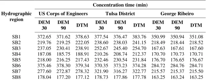
The concentration times obtained by using the three selected methods are assembled in Tables 8 and 9. Table 8 shows the values obtained by using the hydrographic information available for the 1: 50,000 scale information plans. Table 9, on the other hand, presents the values corresponding to the use of hydrography in 1: 250,000 scale information plans.

(10)

Table 8. Concentration times (minutes) obtained from 1:50,000 scale hydrography.

Concentration time (min)

US Corps of Engineers Tulsa District George Ribeiro DEM

30 DEM 90 DTM DEM 30 DEM 90 DTM DEM 30 DEM 90 DTM SB1 372.65 371.62 378.63 377.54 376.47 383.76 350.99 350.94 351.08 SB2 219.76 219.25 222.05 238.60 238.03 241.15 218.49 218.44 218.52 SB3 237.05 230.41 238.91 252.67 245.40 254.70 167.63 167.61 167.60 SB4 187.08 185.75 188.91 210.26 208.74 212.37 170.70 170.73 170.71 SB5 218.00 216.25 217.43 232.46 230.54 231.84 176.70 176.65 176.67 SB6 375.46 378.30 379.34 370.35 373.23 374.28 284.72 284.76 284.71 SB7 277.60 272.87 278.32 321.90 316.27 322.77 215.57 215.37 215.50 SB8 178.04 177.20 177.12 178.73 177.86 177.78 163.25 163.24 163.25

Table 9. Concentration times (minutes) obtained from 1:250,000 scale hydrography.

Concentration time (min)

US Corps of Engineers Tulsa District George Ribeiro DEM

30 DEM 90 DTM DEM 30 DEM 90 DTM DEM 30 DEM 90 DTM SB1 359.31 356.15 363.41 372.68 369.32 377.06 332.98 332.94 332.96 SB2 217.10 215.72 218.94 238.74 237.18 240.81 214.45 214.45 214.46 SB3 234.81 226.20 235.81 250.12 240.71 251.22 166.44 166.41 166.42 SB4 183.71 181.50 185.01 208.35 205.79 209.87 167.54 167.53 167.53 SB5 216.46 213.09 215.40 231.37 227.67 230.20 177.32 177.29 177.26 SB6 371.81 371.06 374.37 369.17 368.40 371.77 283.54 283.59 283.52 SB7 257.04 251.62 257.40 310.14 303.43 310.59 192.38 192.48 192.40 SB8 175.24 174.03 174.31 176.97 175.72 176.01 160.60 160.59 160.59

In order to evaluate concentration time-value variations, a reference scenario was established, corresponding to the concentration times obtained from the information plans presenting larger scale or resolution and by the method applicable considering all criteria. This scenario was composed by the concentration time determined by the George Ribeiro method (method usually employed in urban drainage studies in Brazil), using 1:50,000 scale hydrography and digital terrain model appropriated from the 20-meter equidistant contours (sources with higher levels of detailing for hydrography and digital terrain model).

The concentration time percentage value variations in relation to the reference scenario are shown in Table 10.

The values presented in Table 10 indicate that the different concentration time method combinations (US Corps of Engineers. Tulsa District and George Ribeiro) used for hydrography description scale (1: 50,000 and 1: 250,000) and local relief description alternatives (DEM 30 m. DEM 90m and DTM) produced values that varied from approximately -11% (underestimation associated with SB7 when compared to the referential scenario, when using the George Ribeiro method and 1: 250,000 hydrography) and + 52% (overestimate for SB3, Tulsa District method and 1: 50,000 hydrography).

(11)

estimation method, did not produce variations greater than 6%, regardless the analyzed combination; and c) the concentration time appropriation methods, maintaining relief and hydrography representation forms, produced maximum variations greater than 50% (variations estimated for SB7, when considering errors referring to Tulsa District and George Ribeiro methods).

Table 10. Percentage variations in relation to the referential scenario.

Hydrographic

basin Hydrography

Percentage Variations

US Corps of Engineers Tulsa District George Ribeiro

DEM 30 m

DEM

90 m DTM

DEM 30 m

DEM

90 m DTM

DEM 30 m

DEM

90 m DTM

SB1

1:50.000

6.15 5.85 7.85 7.54 7.23 9.31 -0.03 -0.04

Reference Scenario

SB2 0.57 0.34 1.62 9.19 8.93 10.36 -0.01 -0.04 SB3 41.44 37.47 42.55 50.76 46.42 51.97 0.02 0.00 SB4 9.59 8.81 10.66 23.17 22.28 24.41 0.00 0.01 SB5 23.39 22.40 23.07 31.58 30.49 31.23 0.02 -0.01 SB6 31.88 32.88 33.24 30.08 31.09 31.46 0.01 0.02 SB7 28.82 26.62 29.15 49.38 46.76 49.78 0.03 -0.06 SB8 9.06 8.55 8.50 9.48 8.95 8.90 0.00 0.00

SB1

1:250.000

2.34 1.44 3.51 6.15 5.20 7.40 -5.15 -5.17 -5.16 SB2 -0.65 -1.28 0.19 9.25 8.54 10.20 -1.86 -1.86 -1.86 SB3 40.10 34.96 40.70 49.24 43.62 49.89 -0.70 -0.71 -0.71 SB4 7.61 6.32 8.38 22.05 20.55 22.94 -1.86 -1.86 -1.86 SB5 22.52 20.62 21.92 30.96 28.87 30.30 0.37 0.35 0.33 SB6 30.60 30.33 31.49 29.67 29.40 30.58 -0.41 -0.39 -0.42 SB7 19.28 16.76 19.44 43.92 40.81 44.12 -10.73 10.68 -10.72 SB8 7.35 6.60 6.78 8.41 7.64 7.82 -1.63 -1.63 -1.63

5. CONCLUSIONS

The study identified concentration times appropriation methods applicable to the hydrographic basins that comprise part of the study area, considering soil occupation, area, length and slope of the main talveg characteristics. Among the identified methods, George Ribeiro, Tulsa District and US Corps of Engineers were considered more appropriate, in the order in which they were mentioned.

The estimated concentration times varied up to 11% considering the variables calculated from different information plans and varied up to 52% considering the variables calculated from different concentration times methods. It was also possible to conclude that there is equivalence between Tulsa District and US Corps of Engineers equations for the hydrographic study basin, and that change of information source related to relief and hydrography did not significantly affect the concentration times appropriation. The adequate concentration times values large importance for drainage systems design and the differences in results obtained by different models in this study shows the importance of field surveys for obtaining information that could contribute to model choice and calibration.

6. BIBLIOGRAPHIC REFERENCES

BRASIL. Departamento Nacional de Infra-Estrutura de Transportes – DNIT. Manual de Hidrologia Básica para Estruturas de drenagem. Rio de Janeiro, 2005.

(12)

DHAMI, B. S.; PANDEY, A. Comparative review of recently developed hydrologic models. Journal of Indian Resources Society, v. 33, n. 3, p.34-42, 2013.

FAN, F. M.; COLLISCHONN, W. Integração do modelo MGB-IPH com sistema de informação geográfica. Revista Brasileira de Recursos Hídricos, v. 19, n. 1, p. 243-254, 2014.

FARIAS JUNIOR, J. E. F.; BOTELHO, R. G. M. Análise comparativa do tempo de concentração: estudo de caso rio Cônego, município de Nova Friburgo/RJ. In: SIMPÓSIO BRASILEIRO DE RECURSOS HIDRÍCOS, 19, 2011. Anais... Maceió: Associação Brasileira de Recursos Hídricos, 2011. 1 CD-ROM.

FERRAZ, F. F. B.; MILDE, L. C. E.; MORATTI, J. Modelos hidrológicos acoplados a sistemas de informações geográficas: um estudo de caso. Revista de Ciência & Tecnologia, v. 7, n. 14, p. 45-56, 1999.

FITZ, P. R. Geoprocessamento sem complicação. São Paulo: Oficina de Textos, 2008. GRECCO, L. B.; MANDELLI, M. S.; REIS, J. A. T.; MENDONÇA, A. S. F. Influência da

Seleção de Variáveis Hidrológicas no Projeto de Sistemas Urbanos de Macrodrenagem –

Estudos de Caso para o Município de Vitória – ES. Revista Brasileira de Recursos Hídricos, v. 17, n. 4, p. 197-206, 2012.

HALWATURA, D.; NAJIM, M. M. M. Application of HEC-HMS model for runoff simulation in a tropical catchment. Environmental Modelling & Software, v. 46, p. 155-162, 2013. INSTITUTO CAPIXABA DE PESQUISA, ASSISTÊNCIA TÉCNICA E EXTENSÃO RURAL - INCAPER. Hidrometeorologia. 2011. Disponível em: http://hidrometeorologia.incaper.es.gov.br/caracterizacao/cacho_itap_carac.php. Acesso em: 13 abr. 2012.

MATA-LIMA, H.; VARGAS, H.; CARVALHO, J.; GONÇALVES, M.; CAETANO, H.; MARQUES, A. et al. Comportamento hidrológico de bacias hidrográficas:integração de métodos e aplicação a um estudo de caso. Revista da Escola de Minas, v. 60, n. 3, p. 525-536, 2007.

MCCUEN, R. H.; WONG, S. L.; RAWLS, W. J. Estimating urban time of concentration. Journal of Hydraulic Engineering, v. 110, n. 7, p. 887-904, 1984. https://doi.org/10.1061/(ASCE)0733-9429(1984)110:7(887)

PAIVA, J.B.D.; PAIVA, E. M. C. D. (Org.). Hidrologia aplicada à gestão de pequenas bacias hidrográficas. Porto Alegre: ABRH, 2001.

PORTO, R. et al., Drenagem urbana. In: TUCCI, C. E. M. (Org.). Hidrologia: ciência e aplicação. Porto Alegre: ABRH, 2014.

PRUSKI, F. F.; BRANDÃO, V. S.; SILVA, D. D. Escoamento superficial. Viçosa: Editora UFV, 2004.

(13)

SHUSTER, W. D.; PAPPAS, E. Laboratory simulation of urban runoff and estimation of runoff hydrographs with experimental curve numbers implemented in USEPA SWMM. Journal of Irrigation and Drainage Engineering, v. 137, n. 6, p. 343-351, 2010. https://doi.org/10.1061/(ASCE)IR.1943-4774.0000301

SILVA, M. M. G. T.; WEERAKOON, S. B.; HERATH, S. Modelling of event and continuous flow hydrographs with HEC-HMS: case study in Kelani River Basin, Sri Lanka. Journal of Hydrologic Engineering, v. 19, n. 4, p. 800-806, 2014. https://doi.org/10.1061/(ASCE)HE.1943-5584.0000846

SILVEIRA, A. L. L. Desempenho de fórmulas de tempo de concentração em bacias urbanas e rurais. Revista Brasileira de Recursos Hídricos, v. 10, n. 1, p. 5-23, 2005.

VINAGRE, M. V. A.; LIMA, A. C. M.; LIMA JUNIOR, D. L. Estudo do comportamento hidráulico da bacia do Paracuri em Belém (PA) utilizando o programa Storm Water Management Model. Engenharia Sanitária e Ambiental, v. 20, n. 3, 2015.