4D waypoints based optimal trajectory generation for unmanned aerial vehicles

UNIVERSIDADE DA BEIRA INTERIOR

Engenharias

4D Waypoints Based Optimal Trajectory

Generation for Unmanned Aerial Vehicles

Tiago Alexandre Gameiro

Dissertação para obtenção do Grau de Mestre em

Engenharia Aeronáutica

(2º ciclo de estudos)

Orientador: Prof. Doutor Kouamana Bousson

ii

iii

Acknowledgments

I would like to express my gratitude to my family who always supported me, giving me the motivation I needed to continue specially in the hardest moments. Also, I would like to thank my friends that stood up by my side during this long journey.

A special appreciation to Professor Kouamana Bousson, my supervisor, for the guidance, support and inspiration he gave me to complete this work.

iv

v

Resumo

Os constantes desenvolvimentos tecnológicos observados recentemente em veículos aéreos não tripulados permitem o seu uso nas mais diversas actividades. Com o aparecimento de novas oportunidades surgem também novos desafios. Atualmente a navegação utilizada limita-se apenas ao seguimento de pontos pré-definidos no espaço, waypoints, utilizando parâmetros de voo no seu controlo.

Este trabalho propõe um método alternativo, que consiste em criar trajectórias a partir de

waypoints em 4D, ou seja, com três coordenadas espaciais e uma quarta temporal. Assim, é

possível antever o percurso e garantir que se encontra no local pretendido no tempo certo. Como passar pela posição exata de um waypoint é muitas vezes difícil e excusado, utiliza-se uma tolerância em redor deste, proporcionando a passagem na vizinhança definida por uma esfera com o raio igual a essa mesma tolerância. Neste trabalho é proposto um algoritmo que encontra o ponto tridimensional no interior dessa esfera que minimiza o comprimento do trajecto entre o waypoint anterior e o seguinte.

A trajetória por sua vez é definida interpolando as coordenadas dos waypoints através de um polinómio de ordem cinco. Desta forma é possível restringí-la de modo a criar uma trajectória cujos parâmetros de voo cumprem os limites de navegação associados ao veículo.

Utilizando dados de um veículo aéreo não tripulado de pequenas dimensões, foi possível criar uma trajetória definida por waypoints 4D com um comportamento regular e bastante suave. O percurso escolhido consiste num loiter em hipódromo definido por seis waypoints cujo tempo foi definido de modo a tentar manter de uma velocidade constante em todo o percurso. A simulação foi realizada com sucesso, sendo os limites impostos respeitados ao longo de todo o domínio de tempo.

Desta forma comprova-se a possibiliadde da criação de trajetórias a partir de waypoints 4D específicas para cada veículo aéro não tripulado, gerando assim uma nova área de oportunidades para missões em que o tempo é um factor crítico, ou onde a forma do percurso é crucial.

Palavras-chave

vi

vii

Abstract

The constant technological developments recently observed on unmanned aerial vehicles allow its use on diverse activities. With the arrival of new opportunities new challenges arrive as well. Nowadays the navigation methods used is limited to following pre-defined points in space, waypoints, by using the flight parameters values in its control.

This work proposes an alternative method, consisting in creating trajectories from 4D waypoints, i.e. three spatial coordinates plus a temporal one. So, it is possible to foresee the path e guarantee that it will be on the desired place at the right time.

Because passing through the exact position of a waypoint is rather difficult and not always required, a tolerance is used around it, allowing the passage on the vicinity defined by a sphere whose radius is equal to that tolerance. In this work an algorithm is proposed to find the tridimensional point in the interior of that said sphere which minimizes the path length between the previous and next waypoint.

The trajectory is defined interpolating the waypoint coordinates, using a fifth order polynomial function. This way, it is possible to constrain said function in order to create a trajectory whose flight parameters comply with navigation limits associated with the vehicle. By using the limits associated with a small unmanned aerial vehicle, it was possible to create a trajectory defined by 4D waypoints with a consistent behavior and quite smooth. The path chosen is a Racetrack Pattern loiter defined by six waypoints whose time was defined in order to attempt to maintain a constant velocity through the path. The simulation was a successfully performed, being the limits imposed respected through the entire domain of time.

Therefore, the possibility of creating 4D waypoint based trajectories is proven, generating a new area of opportunities for time based missions where time plays a critical role, or the shape of the path is crucial.

Keywords

viii

ix

Contents

Table list... xiii

Nomenclature... xv 1. - Introduction... 1 2. - Problem modeling... 5 2.1. -Coordinate transformation... 5 2.2. -Waypoint optimization... 5 2.3. - Slope computation... 7 2.4. - Flight constraints... 8 2.5. - Polynomial functions... 9

3. - Simulation and results... 11

3.1. – Dynamics constraints... 11

3.2. – Case studies... 12

3.2.1. - Racetrack Pattern loiter... 12

3.2.1.1. - Trajectory generation... 14 3.2.2. – General path... 20 3.2.2.1. – Trajectory generation... 21 4. -Conclusion... 26 3.1. – Contributions... 26 3.2. - Future work... 26 References... 28

x

xi

Figure list

Figure 1.1 – Navigation through 4D waypoints... 2

Figure 3.1 – Racetrack Pattern loiter... 12

Figure 3.2 – Map with the waypoints for the Racetrack Pattern loiter... 13

Figure 3.3 – 3D trajectory for the racetrack Pattern loiter... 14

Figure 3.4 – Velocity function... 15

Figure 3.5 – Acceleration function... 16

Figure 3.6 – Yaw rate function... 17

Figure 3.7 – Flight path function... 17

Figure 3.8 – Flight path rate function... 18

Figure 3.9 – Roll function... 19

Figure 3.10 – Roll rate function... 19

Figure 3.11 – Map with the waypoints for the Racetrack Pattern loiter... 20

Figure 3.12 – 3D trajectory for the racetrack Pattern loiter... 21

Figure 3.13 – Velocity function... 22

Figure 3.14 – Acceleration function... 23

Figure 3.15 – Yaw rate function... 23

Figure 3.16 – Flight path function... 24

Figure 3.17 – Flight path rate function... 24

Figure 3.18 – Roll function... 25

xii

xiii

Table list

Table 3.1 - Limits of the UAV... 11 Table 3.2 - Geodetic coordinates for the Racetrack Pattern loiter... 14 Table 3.3 - Geodetic coordinates for the Racetrack Pattern loiter... 21

xiv

xv

Nomenclature

γ Flight path angle

λ Longitude σ Radius of tolerance φ Latitude Φ Roll angle Ψ Heading a Acceleration e Earth eccentricity

Ea Earth semi-major axis

g Gravitational acceleration

h Altitude

t Time

UAV Unmanned Aerial Vehicle

V Velocity

x, y, z Geocentric coordinates

xvi

1

Chapter 1 - Introduction

Over the last years the use of Unmanned Aerial Vehicles (UAVs) has significantly increased, taking a more prominent role in aerial missions. As new technologies are applied, new opportunities are created for more complex tasks.

With all the potential associated with the constantly emerging new technologies it is possible to see nowadays a vast array of useful applications in which the use of UAVs excel, for either civilian or military operations [1]. An autonomous vehicle is generally the choice for a mission especially if the task in question is risky, dull, dangerous or if there is a cost reduction involved.

Taking into account the increasing number of technologies that constantly enable new operational capabilities of the UAV it is important to increase their level of performance, autonomy, reliability and integration with a controlled airspace full of manned vehicles. To do so, it is necessary to emphasis the mission planning [2] [3], supervision and collision avoidance [4] [5], combining vehicle constraints and mission constraints [6].

With the increasing number of UAVs navigating in the same airspace at the same time, it becomes mandatory to regulate that airspace, by preventing the risk of collision within a network of UAVs. The lack of reliable real-time information about the trajectories and the absence of effective means of communication between them [7] may aggravate this problem. A time based trajectory will become useful in these situations, by preventing the UAVs to occupy the same airspace, at the same time.

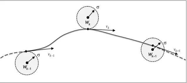
Another advantage of this work relies on the waypoint based navigation. For a UAV to navigate through a set of pre-defined waypoints it can, using a more simple approach, navigate between two consecutive waypoints independently, by controlling the desired heading and flight path angle and adjusting the velocity until it reaches the vicinity of the following waypoint. Then it chooses the next waypoint, and the whole process is repeated. There is no time monitoring over the path produced by the UAV or over the time required to complete the mission. By using 4D waypoints, these are defined by three dimensions in a Cartesian space, plus another one, the time; that means the 4D waypoint is the position in space where the vehicle has to be at a specified time. Let WP represent the 4D waypoint:





 , , ,

WP x y z t

(1.1)

Hence, to create a trajectory where specific points have a time parameter associated, all the points along the path must be defined by a function of time, thus generating a smooth, continuous, optimized path.

2

One of the main advantages of this is the fact that by having this well-defined trajectory and by using a robust controller, the path of the UAV can be defined before its flight with better precision and properly optimizing it for the mission. The use of 4D waypoints opens new possibilities for missions where time is a critical issue. Taking into consideration that UAV have limited time flight time, the opportunity to know exactly the total time used on a mission, is a considerable advantage during the planning process.

During its flight the exact position of the UAV can only be estimated, recurring to sensors such as GPS and inertial measurement units, up to a certain precision. Furthermore, by operating under real world conditions that include, for example, uncertain cross winds, the real final path is rather difficult to determine. For some missions the waypoints chosen are a mere indication of the zone where the UAV should fly over.

For trajectories where the main mission lies between waypoints, and the only purpose they serve are to indicate the zone where the UAV should change direction, their exact position becomes somehow irrelevant. Because this is not always the case and it varies on the mission itself, usually a radius of tolerance is pre-defined. At the specified time for the waypoint the distance to the estimated position of the UAV should be inferior or equal to this radius. By using a trajectory as a function of time it can be optimized by considering the mean direction of both previous and following waypoints. Therefore, for the purposes of the path planning, new positions ought to be calculated in order to reduce its total length, providing as well a smoother trajectory near the waypoints. For UAV such as a winged aircraft with limited turn rates, this is particularly important.

As it is observed in the previous figure (1.1) the chosen point within the sphere of tolerance may lie on the surface of that sphere, shortening the length of the path, or inside, avoiding unnecessary deviations. k v

σ

σ

Figure 1.1 – Navigation through 4D waypoints.

3

For missions where time is a key factor, the use of 4D waypoints is essential. Thus, the only way to assure that the path that connects them continuously and smoothly with respect to the limits to the UAV is to make the path itself a highly constrained function of time. Even though 4D waypoint based trajectories are a relatively new area of research, not much has been done to take in consideration the flight constraints of the UAV and other types of restrictions. Most of the algorithms proposed deal only with the path planning, focusing only on its shape for reference purposes only.

To accomplish so, there are a few approaches possible, from basic polynomial interpolation [8][9] to B-Spline functions [10], such as Bézier curves [11]. This work proposes a slightly different approach to the conventional methods by allowing the time parameter to play an active role in the control of the UAV. Where most works done in this field only allow to the find a trajectory and use its points for guidance, this method allows the creation of one that while respecting the constraints imposed, allowing the UAV to be controlled by directly. One of the main disadvantages associated with the 4D based trajectories is the fact that with all the constraints required to properly define one, there are almost no degrees of freedom to allow optimization.

It is important to refer that through all this work, the algorithm uses only geocentric coordinates that have been previously transformed [12]. The first approach made was to interpolate the Cartesian coordinates with a modified version of the cubic Spline. Those polynomial functions required four coefficients each, which were found by solving a system where four constraints were applied: two for continuity and two for differentiability at the limits of the time domain. Unfortunately, that was not good enough, as there was no room for optimization and the acceleration function was not continue.

Then, following the research that had been applied to path planning in robots and in a few UAVs, the cubic Bézier curves were put to the test. Instead of interpolating each Cartesian coordinate individually, the Bézier curves were able to create a smooth path requiring only two control points that were conveniently chosen as the velocity vectors to assure tangency and continuity at the domain limits. Although it offered the better results with less complexity, it had the same problems with the acceleration. Also, the velocity functions would often exhibit odd patterns, impossible to control.

The solution chosen was to increase the degree of the polynomial function, adding also more constraints. By limiting the acceleration at the domain limits (as well as the velocity), the final system had six coefficients to be found, and six linear equations to solve.

There are a few disadvantages of using this method. One of them is the increase in the complexity of the equations used to verify the limits of the UAV, such as the velocity,

4

acceleration, yaw rate, flight path, flight path rate, roll and roll rate. With the increase in the degree, the equations become substantially larger, taking more time to compute, even though there is no optimization involved.

Another drawback of using high degree polynomial functions is in the fact that there is a loss of smoothness associated. The ideal degree, for either polynomial function or Bézier curve is three, although, it has proven to be insufficient to constrain the trajectory.

This work is divided in three main parts. The first one, Introduction, is where it is summed up all the relevant information about the current state of developments in this particular area. Then, in Chapter 2, Problem modeling is where the algorithms are presented, including all the relevant equations. In Chapter 3, Simulation and results, a trajectory is generated using real values for the waypoints and for the limits of a UAV. The results are discussed and compared to the previously imposed limits. Finally, the Conclusion presents a sum of all the information and results, discussing its importance, and then, Future work, where the challenges of this work are presented with possible solutions.

5

Chapter 2 - Problem modeling

2.1 - Coordinate transformation

Due to the fact that the trajectory generated requires a geocentric coordinates system, the 4D waypoints used have to be transformed from the usual geodetic coordinate system to Cartesian coordinates.

Considering a general point in space,P_gc, defined by its three geodetic coordinates where









gc

P 

 

(2.1)

To transform these coordinates, the following equations ought to be applied:





(2.2)





(2.3)



(2.4)

Being Ea the semi-major axis of Earth and e its eccentricity, n is computed as follows:

2 2 1 sin Ea n e



(2.5)

Once the Cartesian coordinates of the waypoints are computed, the next step is to determine the optimal position in its neighborhood where the final trajectory should pass. As it was referred before, because the UAV is not obliged to truly intercept the exact waypoint, but only to be within an imaginary sphere of radius



2.2 - Waypoint optimization

Given a waypoint W_k, the point within its sphere of tolerance to be chosen is the closest to the imaginary line connecting the waypoints W_k1 to W_k1.





 , ,

k k k k

6

To find the point it is required to project Wk on the plane which includes Wk1 and Wk1, and

whose normal vector lies on the plane which simultaneously comprise W_k, W_k1 and W_k1.

1 k k 1 k k 1 n WW_ W W_

(2.7)

(2.8)













(2.9)

Where  denotes the cross product between two vectors. The optimal solution is the projection of W_k on the plane (2.9). If the distance between these two is equal or inferior to



Considering the projected point W*:

* _(x*_{, ,}* _z*₎T

W  y

(2.10)

In order to make the projection, let following equations describe the line between W_k and

* W :       k k k x x y y z z l a b c

(2.11)



 

 



(2.12)

(2.13)

Hence, accordingly to (2.11), W*is given by:

       * 2 2 2 k k k k ax by cz d x x a a b c

(2.14)

(2.15)

7        * 2 2 2 k k k k ax by cz d z z c a b c

(2.16)

Let the distance between W_kandW*be represented byD:



 

 



  * 2  * 2  * 2

k k k

D x x y y z z

(2.17)

The new point to be considered as the new waypoint can be now defined. If D



 *

k

W W

(2.18)

On the other hand, ifD





(2.19)

2.3 - Slope computation

Once these new points are defined, the value of their slope is computed as the mean value regarding the Cartesian coordinates of the waypoint before and the one after, with the exception of the first and last waypoints.

Letv_kjbe the slope for the W_kwaypoint, and jthe variable.

 

(2.20)

 

(2.21)





(2.22)

Hence, the slope vector at each waypoint W_k is:

( , , )x y z T

k k k k

8

2.4 - Flight constraints

The flight of the UAV under real world conditions is constrained, due to its performance, the structural limits, safety reasons, the mission and other factors. Considering Cartesian coordinates, the constraints to be applied are:

 Velocity, V:  2 2 2 V x y z

(2.24)

(2.25)

Where x, yand z represent the first derivative of the polynomial function for each individual coordinate. It can also be interpreted as the velocity components on each Cartesian axis.  Acceleration, a:  a V

(2.26)

(2.27)





(2.28)



 

(2.29)

 Flight path rate,





 

(2.30)





(2.31)



9



 

(2.32)







(2.33)



 

(2.34)

 Roll rate,





 

(2.35)

2.5 - Polynomial functions

To properly constrain the functions it is needed to set the initial and final position, first and second derivatives to the chosen values. Only this way it is possible to guarantee the continuity of the velocity and acceleration functions across the trajectory. As it was presented before, to define this trajectory a fifth order polynomial is enough. The six coefficients that shape the function can be found by solving a system comprised of six equations. There ought to be a fifth-order polynomial function S_kj for each one of the three Cartesian coordinates between two consecutive waypoints, as follows:

 ₅ 5 ₄ 4 ₃ 3 ₂ 2 ₁  ₀ ( )

j j j j j j j

k k k k k k k

S t C t C t C t C t C t C

(2.36)

For the first derivative,S_kj, could also represent the velocity for the j axis, being





(2.37)

For the second derivative, S_kj, may represent, the acceleration for the j axis, being





(2.38)

10

Therefore, to find the six coefficients for the equation (2.36) it is necessary to define a velocity and acceleration at both starting and ending points. Also, to maintain the continuity over the three coordinates, so the velocity of the UAV is appropriate, the slope vector (2.23) could be used. Even though, it is necessary to change its magnitude to meet the requirements. Let

k cruise

V represent the magnitude of the velocity vector V_kat the waypoint k W : ( ,x y, )z T k k k k V  V V V

(2.39)

(2.40)

By scaling the vector the velocity vector it is guaranteed that its norm is equal to the desired velocity

k cruise

V

.

Regarding the acceleration, in order to maintain a trajectory with a steady velocity, the acceleration at each waypoint is set to zero.

(0,0,0)T

k

a 

(2.41)

Now that all the equations are defined, the system for each coordinate is:

                             5 4 3 2 1 0 5 4 3 2 1 5 4 3 2 5 4 3 2 1 0 5 5 4 3 2 4 3 2 2 3 2 5 4 3 2 1 1 1 1 1 1 4 1 5 4 3 2 20 12 6 4 5 4 j j j j j j j k k k k k k k k k k k k j j j j j j k k k k k k k k k k j j j j j k k k k k k k k j j j j j j j k k k k k k k k k k k k j k k C t C t C t C t C t C W C t C t C t C t C V C t C t C t C a C t C t C t C t C t C W C t C _{   }                         4 3 2 1 5 4 3 2 3 2 1 1 1 1 3 2 1 1 1 1 3 2 20 12 6 4 j j j j j k k k k k k k k j j j j j k k k k k k k k t C t C t C V C t C t C t C a

(2.42)

Thus, between two consecutive waypoints, the trajectory is defined by the six coefficients in the following vector:

5 4 3 2 1 0

( , , , , , )

j j j j j j j T

k k k k k k k

11

Chapter 3 - Simulation and results

3.1 – Dynamics constraints

For the simulations three scenarios are represented, describing a common loiter. This profile, the Racetrack Pattern, is described in NATO’s STANAG 4586 [14].

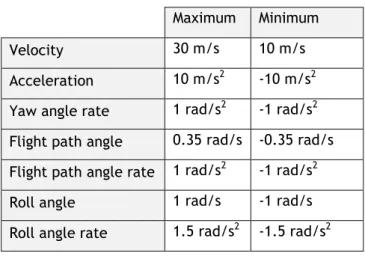
The simulation is computed varying only the waypoints, maintaining the same conditions and limits of the UAV through all of them. Said limits are typical of small UAV, and are presented in the following table:

Table 3.1 - Limits of the UAV

Maximum Minimum

Velocity 30 m/s 10 m/s

Acceleration 10 m/s2 _{-10 m/s}2

Yaw angle rate 1 rad/s2 _{-1 rad/s}2 Flight path angle 0.35 rad/s -0.35 rad/s Flight path angle rate 1 rad/s2 -1 rad/s2

Roll angle 1 rad/s -1 rad/s

Roll angle rate 1.5 rad/s2 _{-1.5 rad/s}2

For the cruising velocity, a value is set, so that the mean value across the trajectory is the same. It is important to point out that the forth coordinate of the waypoints, the time, is determined by setting a random initial value, then solve the system of equations (2.42) and determine the length of the path produced, between two consecutive waypoints using the following equation:  



(3.1)

Hence, the time to use in the next waypoint in order to maintain a mean velocity equal to k cruise V is determined by: 1  k k k k cruise L t t V

(3.2)

V chosen for this simulation is equal to 20 m/s, being the mean value between the minimum and the maximum velocity.

12

 20 /

k cruise

V m s

(3.3)

For the a_k, as it was discussed before, in order to maintain a trajectory with a velocity as close to cruising speed as possible the value is set to equal to 0 m/s2_.

_{0 /} 2

k

a m s

(3.4)

At the waypoints, the tolerance is usually two times or more, bigger than the wingspan of the UAV. So, for this simulation the value of the radius is set to 5m.



(3.5)

After all this, everything is ready to compute the coefficients (2.43) of the polynomial function (2.36).

3.2 – Case studies

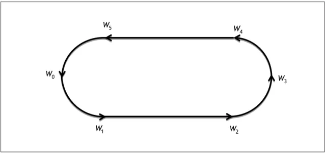
3.2.1 - Racetrack Pattern loiter

This loiter is very common for both manned and unmanned aerial vehicles. It can be used to hold a position or for example to perform some task on the ground below. This trajectory is ideally comprised by two half circles and two straight lines connecting them, as is shown in the following figure:

Typically a cruise velocity is maintained during this time, thus the need to define (3.3). Also the altitude is typically the same through the entire path.

5 W

13

For this pattern a careful choice of waypoints must be made. Each one has an imaginary sphere of tolerance that will alter the final look of the trajectory. Not only that but also the fact that geocentric coordinates are being used. These loiters are projected for geodetic coordinate systems. The geocentric version is slightly different.

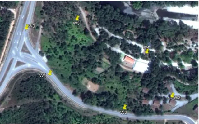
For the simulation, the trajectory chosen is a Racetrack Pattern loiter above the Parque de Campismo de Côja. The waypoints are presented in the following map:

Figure 3.2 – Map with the waypoints for the Racetrack Pattern loiter.

As shown in the figure above, only six different waypoints are required. Between them the algorithm determines the coefficients (2.43) needed.

The geodetic coordinates extracted from Google™ earth are shown in the following table, as the time required for a proper 4D navigation at a constant

k cruise

14

Table 3.2 - Geodetic coordinates for the Racetrack Pattern loiter.

Latitude [º] Longitude [º] Altitude [m] Tempo [s]

0 W 40°16'3.83"N 7°59'56.89"W 240 0 1 W 40°16'1.48"N 7°59'55.26"W 240 4.06 2 W 40°15'59.69"N 7°59'50.27"W 240 10.59 3 W 40°16'0.27"N 7°59'46.91"W 240 14.80 4 W 40°16'2.63"N 7°59'48.54"W 240 19.06 5 W 40°16'4.40"N 7°59'53.53"W 240 25.80

3.2.1.1 - Trajectory generation

Using the equations presented in Chapter 2, the trajectory which passes in the neighborhood of the waypoints is represented in a Cartesian coordinate system in the following figure.

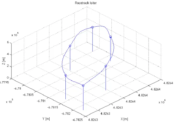
Figure 3.3 – 3D trajectory for the racetrack Pattern loiter.

In the figure (3.3) the curve blue line represents the real path through the different waypoints, starting on the left, descending and going back to the initial point. The vertical

15

markers with the circle on top denote the position of the original waypoints. As it is possible to perceive, the final path comes close to them, but never intercepting them. This is due to the fact that a sphere of tolerance was taken into account. The length of the final path is reduced and the trajectory becomes smoother. This avoids also sharp turns, keeping the UAV further away from its flight limits.

It is important to refer that although the start and end of the path are single point in space, it leads to a cusp. This is caused because the last part of the path does not take into account the hypothetical waypoints ahead (in case of a loop), making the slope computed at that point different.

Simulation results

Regarding the limits imposed to the UAV, structural, aerodynamic, for safety purposes and for the mission itself, as presented before in table (3.1) they ought to be analyzed carefully for the whole length of the trajectory.

Therefore, the velocity, acceleration, yaw rate, flight path, flight path rate, roll and roll rate are represented in the following pages. The figures consist in the functions, in blue, in the time interval between waypoints. They are represented as the vertical lines.

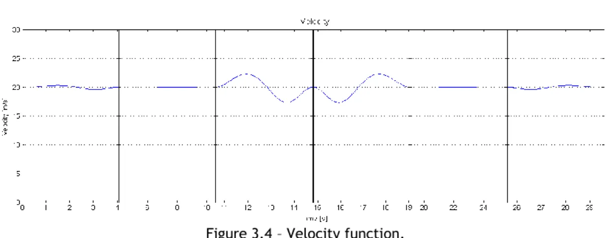
 Velocity:

Figure 3.4 – Velocity function.

As it is possible to see, for a cruise speed of 20 m/s, the function has an overall value like it was intended. For the first three waypoints the deviation from the actual value and the cruise speed is not significant. The same happens to the last three. The fact that this loiter is symmetric makes a noticeable impact on the shape of the trajectory and on the functions associated.

The only real issue with this function is what happens on the half circle of the loiter, where the velocity changes to a local maximum of about 22.5 m/s and a local minimum of about 17.5 m/s, two times. Although these changes make a considerable visual impact, on the

16

steady cruise velocity, the values are perfectly acceptable and far away from the limits imposed.

The velocity function is continuous in the defined domain, and so is its first derivative, as imposed by the system of equations (2.42). Therefore, at each waypoint the function has the same value and slope as the next.

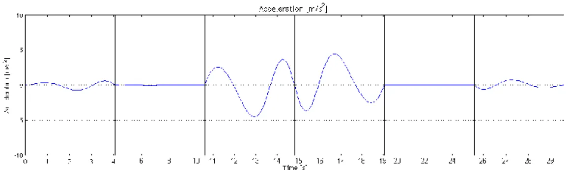
 Acceleration:

Figure 3.5 – Acceleration function.

After analyzing the velocity function, and knowing that the acceleration is nothing more than its first derivative, a function identical in shape is to be expected. In fact, the behavior is alike, even with the steady first and last part of the trajectory, and the middle part where the maximums and minimums are found. As for its values, considering the limits, they represent less than half of it, maintaining a feasible trajectory up to this point. It reaches the maximum of about 0.4 m/s2 _{after the third waypoint, and the minimum of about -0.4 m/s}2 after the next waypoint.

Also, the function is continuous, despite not being differentiable at the waypoints due to the transition between functions.

17

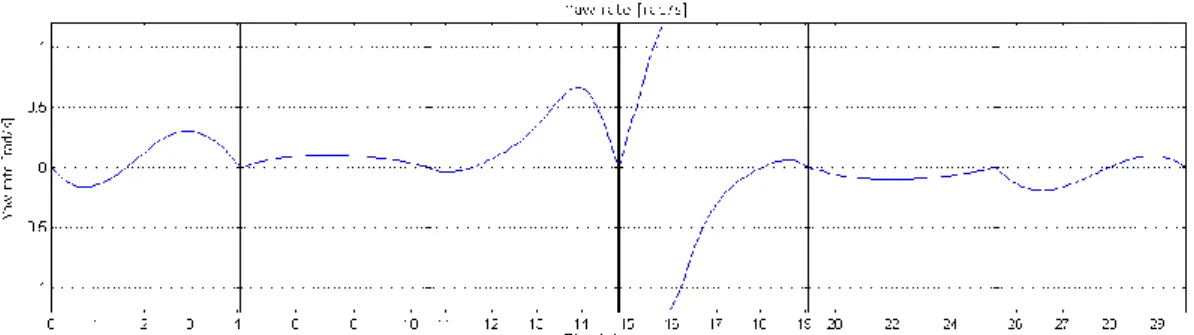
 Yaw rate:

Figure 3.6 – Yaw rate function.

Although the yaw does not have a limit, its rate has. For this particular trajectory, even though that for most of the path the maximum only surpasses half of the value of the superior limit, while doing the turn at the semi-circle, and just reaching about a quarter of the inferior limit also doing a turn, there is a very peculiar situation present.

This situation occurs between the interval [15, 16] seconds, where the yaw just performs a full turn. This triggers an irregular behavior on both functions, leading to an asymptote. Although it leads to values off the charts, it does not imply that the trajectory is not feasible. This is actually a common occurrence under real-world conditions. As a compass completes a full turn, special measures are taken on both hardware and software level to assure that does not compromise the critical systems of both manned and unmanned aerial vehicles.

So, even though there is an asymptote present, providing that this type of situations are accounted for on the controller and at the data acquisition systems, is safe to assume that the trajectory respects the limits imposed.

 Flight path:

Figure 3.7 – Flight path function.

This function presents also a very distinct problem. At first sight it overshoots the limits defined, but upon a closer look at the patterns observed at both the shape of the trajectory

18

and the function itself, an explanation starts to appear. This loiter has constant altitude, but once its coordinates are transformed from geodetic to geocentric, it becomes irrelevant. That is because the shape of the trajectory on a Cartesian plane takes the approximate original form but on a “tilted” plane.

Although the whole trajectory lies on said plane, the flight path angle appears to make reference to another one, resulting in high values which defy the normal values associated with UAVs.

Therefore, it makes it very difficult to properly evaluate the real limits, due to the fact that according to the trajectory represented in the figure (3.3) the flight path angle is very close to zero the whole time, making it the only possible scenario to achieve a planar trajectory. On the other hand, this function presents a maximum and minimum which are about the double allowed by the limits set.

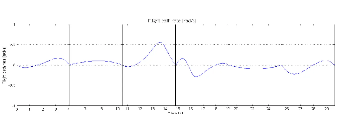
 Flight path rate

Figure 3.8 – Flight path rate function.

Once it was shown that the function for the flight path is not reliable and does not provide viable result under a geocentric coordinates system, it is not pertinent to take the values presented above, even though for the entire time domain it does not exceed the limits defined.

19

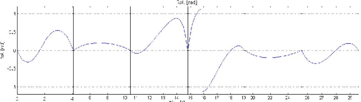
 Roll

Figure 3.9 – Roll function

This function features another asymptote at the same period of time. This is caused because the equation for the roll depends on the value of the heading. So, like before, with the exception of that peculiar moment, the function has local maximums and minimums that do not exceed the limits imposed, with a minimum of about -0.4 rad and a maximum of about 0.8 rad.

 Roll rate

Figure 3.10 – Roll rate function.

This function has no continuity between the waypoints. Nevertheless, with the exception of the asymptote found at the middle waypoint (t=14.8s), resulting from the odd shape of the roll function, the rate of roll does not exceed the limits which are set for a maximum of 1 rad/s and a minimum of -1 rad/s, even though almost reaching that values several times, at both start and end intervals.

20

3.2.2 - General path

Although loiters are frequently the central part of the typical missions assigned to UAVs, the path that leads to the zone where the mentioned loiter is to be performed cannot be overlooked. It may include a starting or final waypoint associated with a low velocity and low altitude in order to perform a take-off or a landing. A varying altitude profile to deal with the terrain morphology is also common.

For this path a landing approach is going to be taken. It features a starting point close to the previous loiter, and then proceeds to follow the nearby river, in order to not fly over populated areas, concluding its flight in an airfield 1860 meters away from the start.

For the flight, a cruise speed will be maintained, although at the end the speed is inferior, as the UAV approaches the landing zone.

At each waypoint, a radius for the sphere of tolerance is used as well. The coordinates system used is the geocentric one, so a transformation of coordinates is required too.

The path chosen is represented in the following figure:

Figure 3.11 – Map with the waypoints for the trajectory.

As shown in the figure above, five different waypoints are used. Between them the algorithm determines the coefficients (2.43) needed.

The geodetic coordinates extracted from Google™ earth [13] are shown in the following table, as the time required for a proper 4D navigation.

21

Table 3.3 - Geodetic coordinates for the trajectory. Latitude [º] Longitude [º] Altitude [m] Tempo [s]

1 W 40°16'3.77"N 7°59'39.08"W 240 0 2 W 40°16'10.35"N 7°59'20.64"W 235 24.10 3 W 40°16'23.71"N 7°59'6.74"W 230 50.56 4 W 40°16'32.86"N 7°58'48.15"W 230 76.87 5 W 40°16'30.09"N 7°58'28.01"W 227 114.38

3.2.2.1 -Trajectory generation

Using the equations presented in Chapter 2, the trajectory which passes in the neighborhood of the waypoints is represented in a Cartesian coordinate system in the following figure.

22

In the figure (3.12) the path is represented by the blue line, being the small blue circles the indication of the position of the waypoints. Due to the extent of the final path, the tolerance near the waypoints is barely noticeable.

In this trajectory, it is clear that this algorithm produces a smooth path, with constant curves avoiding sharp turns. This is particularly important to the landing approach.

Navigation parameters

As presented before in table (3.1) the navigation parameters ought to be carefully analyzed. Therefore, the velocity, acceleration, yaw rate, flight path, flight path rate, roll and roll rate are represented in the following pages. The figures consist in the functions, in blue, in the time interval between waypoints. They are represented as the vertical lines.

 Velocity:

Figure 3.13 – Velocity function.

In this figure, as it was predicted, due to the extent of the path, and the smoothness associated, between the four initial waypoints, the cruise velocity hardly changes. In fact, the maximum and minimum of those functions correspond to about 1% deviation for the value set, 20 m/s.

On the last waypoint, as the landing speed was set to 10 m/s, the transition was progressive, being the maximum the initial value, 20 m/s, and the minimum value 10m/s.

23

 Acceleration:

Figure 3.14 – Acceleration function.

These results are consistent with the velocity shown before, as there is little change during the first four waypoints, where the cruising speed is constant. In this period of time, the maximum value is about 0.2 m/s2_{, and the minimum is about -0.2 m/s}2_.

In the last, part, due to the decrease of velocity, there is a minimum of almost – 0.8 m/s2_. The function is continuous, despite not being always differentiable at the waypoints due to the transition between functions.

 Yaw rate:

Figure 3.15 – Yaw rate function.

The yaw rate function produces good results, in contrast with the previous simulation. In this case, the maximum is about 0.05 rad/s and the minimum is -0.05 rad/s. This is expectable due to the long path.

24

 Flight path:

Figure 3.16 – Flight path function.

As before, in figure (3.7), the flight path does not present conclusive results. Again, by looking at the values and the limits, an overshooting is obvious. One of the ways to really estimate the flight path is looking at the results produced by a geodetic approach. Unfortunately, that is not possible. One possible solution relies on estimating the mean flight path between waypoints. Considering that the altitude is interpolated, and knowing that in this particular trajectory the mean altitude step between waypoints that are hundreds of meters apart is 5 meters, we can expect that the flight path is not exceeded.

Even so, the maximum of this function is 0.7 rad and the minimum of about -0.4 rad.

 Flight path rate

Figure 3.17 – Flight path rate function.

As expected, the results show almost no change during the entire time, with a maximum of about 0.05 rad/s and a minimum of almost -0.05 rad/s.

25

 Roll

Figure 3.18 – Roll function

This function has a maximum of about 0.08 rad and a minimum of -0.08 rad, both after the second waypoint. Besides that, the function values are close to zero the whole time.

 Roll rate

Figure 3.19 – Roll rate function.

As expected, the deviation from zero in this function is about 2.5% of the limits, both positive and negative. The maximum is 0.025 rad and the minimum is -0.25 rad, both at the second waypoint.

26

Chapter 4 - Conclusion

With this work several steps were made in order to achieve a complete algorithm capable to create trajectories from 4D waypoints. With the sphere of tolerance, an optimal point was found for each waypoint. It was done recurring to geometrical properties ensuring that it would minimize the distance between both previous and following waypoints. If the waypoints were not almost aligned, which is rarely the case, the point would be found on the surface of the sphere. This operations lead to a smother final trajectory with a reduced path length. This was achieved without recurring to iterative processes, reducing the time and computational load usually required.

4.1 – Contributions

By using a geocentric coordinates system, different equations had to be used in order to find the state variables, even though with results that are not always the expected, specially the flight path angle. Even so, by analyzing the results from the other equations, it is possible to assume that the trajectories produced by these algorithms are ready to be tested in real world conditions, once a proper controller is applied. For the simulated cases, the results, when valid and ignoring peculiar situations like the yaw angle situation, meet the trajectory specifications.

These algorithms can be applied to any set of 4D waypoints. It is also important to refer that these trajectories do not depend on the vehicle constraints themselves, as they only exist to be checked once the trajectory is created. In order to comply with the limits, a careful choice of waypoints is advised. As it is seen in the trajectory generated, the further apart are two waypoints, the smoother the path will be, avoiding also situations where the parameters are pushed to the limit.

As it was possible to see by the last simulation, by considering a general trajectory, where the UAV is not pushed to the limits, the results prove that this algorithm is very versatile, able to handle diverse types of situations, proving to be suitable candidate to perform new types of missions designed for UAVs.

4.2 - Future work

Although the algorithm has proven reliable, by creating feasible trajectories under several constraints, there is still room from improvement.

27

It is possible to create trajectories for other mission profiles, moving from a velocity fixed approach to other parameters.

Polynomial functions of higher degrees are able to allow more constraints, or more room for optimization, such as minimum path length or minimal fuel consumption, (although they may become less smooth) and require more time achieve those results.

Other critical issue is the control of the UAV to follow these trajectories. Due to the fact that the control variables are not fixed reference values, but instead functions of time, a custom developed controller may be required. This also comes from the fact that, for example, if by controlling the velocity, any disturbance may change its value. The controller not only had to stabilize to the proper value, but also reduce or increase the velocity by an exact amount so that the UAV would not arrive at the waypoint to soon.

28

References

[1] Bortoff, S. A., “Path Planning for UAVs”, Proceedings of the American Control

Conference, Chicago, IL, U.S.A., 2000, pp. 364-368.

[2] Ruz, J. J., Arévalo, O., Pajares, G. and Cruz, J. M., “UAV Trajectory Planning for Static and Dynamic Environments”, Aerial Vehicles, T. M. Lam, Ed. InTech, 2009, pp. 581-600.

[3] Roberge, V., Tarbouchi, M. and Labonté, G., “Comparison of Parallel Genetic Algorithm and Particle Swarm Optimization for Real-Time UAV Path Planning”, IEEE Transactions On

Industrial Informatics, Vol. 9, No. 1, 2013, pp. 132-141.

[4] Sigurd, K., How, J, “UAV Trajectory Design using Total field Collision Avoidance”, AIAA

Guidance, navigation and Control Conference and Exhibit, Austin, TX, U.S.A., 2003.

[5] Han, S. and Bang, H., “Proportional Navigation-Based Optimal Collision Avoidance for UAVs” International Journal of Control, Automation and Systems, 2009, Volume 7, Issue 4, pp. 553-565.

[6] Gutiérrez, P., Barrientos, A., Cerro, J. and San Martín, R., “Mission planning and simulation of unmanned aerial vehicles with a GIS-based framework”, AIAA Guidance,

navigation and Control Conference and Exhibit, Keystone, CO, U.S.A., 2006.

[7] Frew, E. W. and Brown, T. X., “Networking issues for small unmanned aircraft systems,”

Journal of Intelligent and Robotic Systems, vol. 54, 2008, pp. 21–37.

[8] Barrientos, A., Gutiérrez, P. and Colorado, J. “Advanced UAV Trajectory Generation: Planning and Guidance”, Aerial Vehicles, T. M. Lam, Ed. InTech, 2009, pp. 55-82.

[9] Lau, L., Sprunk, C. and Burgard, W., “Kinodynamic Motion Planning for Mobile Robots Using Splines”, Intelligent Robots and Systems Conference, St. Louis, MO, U.S.A., 2009. [10] Arney, T., “Dynamic Path Planning and Execution using B-Splines”, Information and

Automation for Sustainability Conference, Melbourne, VIC, Australia, 2006.

[11] Douglas, G. M., Neto, A. A. and F. M. C., Mário, “Feasible UAV Path Planning Using Genetic Algorithms and Bézier Curves” Advances in Artificial Intelligence, 2010, Vol. 6404, pp. 223-232.

[12] Vermeille, H., “Computing geodetic coordinates from geocentric coordinates”, Journal

29

[13] 2013 Google Inc., Google Earth 7.1.1.1888. (Visited on September 2013). [14]NATO, STANAG 4586, Edition 2.5, 2007.