Computational tool for modelling performance of photovoltaic panels

(1)

INTERNATIONAL CONFERENCE ON ENGINEERING UBI2011 - 28-30 Nov 2011 – University of Beira Interior – Covilhã, Portugal

Computational

tool

for

simulating

the

performance of photovoltaic panels

Romeu Santos 1_{, Pedro Dinis Gaspar} 2

1,2_{University of Beira Interior, Faculty of Engineering, Department of Electromechanical Engineering}

1

r_santos14@hotmail.com; 2 dinis@ubi.pt

Conference Topic – CT 9 Abstract

An accurate model based on Shockley equation is used to simulate photovoltaic modules. This article proposes the use of double exponential model to simulate the electrical characteristics of any photovoltaic panel on market. The modeling tool allows the analysis of the behaviour of electrical characteristics in accordance with environmental changes such as temperature and irradiance. It is verify that these extrinsic factors influence the photovoltaic efficiency.

Keywords: Photovoltaic Cells; Modeling; Simulation; MATLAB; I-V and P-V Curves.

1. Introduction

The basic unit for converting solar energy into useful electrical energy is the solar cell. Grouped cells form photovoltaic (PV) modules with the aim of increasing energy production and make the process more practical. The electrical characteristics electrical current-voltage (I-V) and electrical power-voltage (P-V) of PV systems are not linear and depend on solar radiation and temperature.

The double exponential model is composed of a series resistance, parallel resistance (shunt), two saturation currents, a photovoltaic current and ideality factor. This model offers greater accuracy than a single exponential model, which only makes use of a series resistance, a diode and a shunt resistance. The later resistance is usually neglected as indicated by Ishaque et al. [1-3]. Thereby it is necessary a tool to extract all the parameters that characterize the PV modules for subsequent layout of I-V and P-V curves, independently of the module to simulate [4].

2. Modeling Photovoltaic Systems

The use of an electrical equivalent circuit makes possible modelling the electrical characteristics of a photovoltaic solar cell. To accomplish this task it is necessary to know the best way for modeling and further implementation in MATLAB. This same technique is applicable in modeling of PV modules as described by Oi [5].

2.1. Simple Model of Solar Cell

The simplest equivalent circuit representative of a solar cell is given by a current source in parallel with a diode. The source output is directly proportional to the incident light and temperature in the cell [6-7]. The current source represents the current generated by photons (too often called Iph or Il). During the night or in the dark, the solar cell is not an active device, works like a p-n diode junction, which generates little current. However, if connected to an external source (high voltage) generates a current Id, called diode current [4]. The diode determines the I-V characteristics of the cell [7].

There are two key parameters often used to characterize PV cells, are they short-circuit current (Isc) and open circuit voltage (Voc).

(2)

(a) (b)

Figure 1 – Diagrams of the conditions in (a) short-circuit and (b) open circuit [5].

Closing the terminals of a photovoltaic cell (Fig. 1a), the current generated by photons that will flow out, is called short-circuit current (Isc). Thus, Iph = Isc. When the connection of the terminals circuit is not established (open circuit), the current generated by photons is closed internally by the intrinsic p-n junction of the diode (Fig. 1b). This condition provides an open circuit voltage (Voc) [5-6].

The output current (I) of the solar cell (Eq. 1) can be determined by applying Kirchhoff’s laws in the equivalent circuit (Fig. 2) [5]. The diode current Id (Eq. 2) is given by Shockley’s equation [5, 8].

(1)

- (2)

(a) (b)

Figure 2 – Photovoltaic cell (a) loading and (b) the simple equivalent circuit [5].

2.2. High Accuracy Model

There are some effects that should be considered in the simplest model to obtain more accurately the I-V characteristics of the solar cell [5].

They are: the series resistance (Rs), which induces a current through the semiconductor material, the metal mesh, the shunt resistance (Rsh), among others [5, 9]. These losses are associated with a small leakage current associated with a resistive path in parallel with the intrinsic device [5, 9]; recombinations in photovoltaic cells area promote the reduction of non-ohmic currents routes in parallel with the intrinsic solar cell. This condition is relevant for low bias voltages and can be represented in a equivalent circuit through a second term in a diode density current (Is2), which is different from the current density of an ideal diode, which usually gives an ideality factor (a) with a different value of 1 and a maximum value of 2 [5, 9]. Summarizing these effects, the I-V relationship can be described by:

* ( )₊_*( )_{+ (} ) (3) (4)

(3)

INTERNATIONAL CONFERENCE ON ENGINEERING UBI2011 - 28-30 Nov 2011 – University of Beira Interior – Covilhã, Portugal Equation 3 is called a double exponential equation, where Vt (Eq. 4) is the thermal voltage of the p-n junction. This equation provides the I-V characteristic curve (Fig. 3), where the three most important points are represented: short-circuit point (Isc, 0); maximum power point, MPP (Imp, Vmp), and open circuit voltage point (0, Voc) [10-11]. These authors also suggest that Equation 5 should be used to obtain the better I-V characterization for cells made of amorphous silicon. This equation comes from the double exponential equation by setting the saturation current Is1 = 0. Both equations are not linear, making it difficult to determine an analytical solution [12].

Figure 3 – I-V characteristic curve of a photovoltaic device and the three remarkable points: short-circuit current (0,Isc), MPP (Vmp,Imp), and open circuit voltage (Voc,0) [10-11].

- * (

)_{- + -}

(5)

Equations 3 and 5 describe the equivalent circuits that represent these relationships. The circuit of the double exponential model, corresponding to Equation 3, is shown in Fig.4a and the circuit of the simple exponential model, corresponding to Equation 5 is illustrated in Fig. 4b.

Figure 4 – (a) Double exponential model and (b) simple exponential model of a PV cell [1-3, 13].

Therefore, modelling PV modules primarily involves the estimation of nonlinear I-V curves. Researchers have used circuit topologies to model the electrical characteristics of PV modules when subject to variations such as irradiance and temperature. By far the simplest approach is the simple exponential model, i.e. a current source in parallel with a diode. An improvement of this version is the consideration of a series resistance (Rs) [1-3]. However, the model remains very simple, exhibiting serious shortcomings when subjected to high temperature variations, due to the non introduction of the open voltage coefficient (kv) [7]. An extension of the simple exponential model further includes a shunt resistance (Rsh).

(4)

INTERNATIONAL CONFERENCE ON ENGINEERING UBI2011 - 28-30 Nov 2011 – University of Beira Interior – Covilhã, Portugal Including this resistance, the number of parameters increases to five, increasing its complexity but also increasing the accuracy of the results [1-3, 14-15].

The models behave like a “black box” (Fig. 5), so systems designers use environmental parameters such as irradiance, G, and temperature, T, in order to study the system conversion to any fixed point or variable with respect to these parameters. It is necessary to relate the five variable parameters of the equation with the two environmental parameters (G, T) [12].

The simple exponential model is based on a formulation where the recombination losses are disregarded. In a real solar cell, recombination represents substantial losses, but is not adequately modeled by simple exponential model. This loss can be considered in the double exponential model. However, the inclusion of a diode increases the calculation parameters from five to seven, where the latter is the Is2 and a2 [1-3].

Figure 5 – Basic process of modeling PV panels [12].

2.3. Modeling of a Photovoltaic Module

The modeling strategy for a photovoltaic module is not very different from the modeling of a photovoltaic cell. The model is similar, consider the same parameters, however the parameter open circuit voltage (Voc) is different and must be divided by the number of existing cells in the module [5]. In this particular study, we use the double exponential model for modeling of a PV panel in order to reduce the computational error propagation [1-3]. Therefore, using this model offers a more accurate calculation compared to others. In particular, the double exponential model is a preferred choice, but it is necessary to take into account the most demanding computational calculations [1-3, 16].

The manufactures of PV modules provide access to few experimental data about the thermal and electrical characteristics. Unfortunately, some of the parameters required for modeling PV modules cannot be found in the manufacturer’s datasheets, such as the current generated by light, series and shunt resistances, diode ideality constant, reverse saturation current and energy of the band gap of the semiconductor. All datasheets of photovoltaic modules have information concerning the: nominal open circuit voltage (Voc,n); nominal short circuit current (Isc,n); voltage in the MPP, (Vmp); current in the MPP (Imp); temperature coefficient of the open circuit voltage (kv); temperature coefficient of the short-circuit current (ki), and maximum experimental peak power (Pmax,e). This information is provided with reference to the standard test conditions (STC) for temperature and irradiance [10-11].

Therefore, upon making use of the double exponential model, should obey to Equation 3 and the circuit of Figure 4 to perform the modeling and the I-V characterization. For this, other equations are required to find the parameters needed for modeling: Iph, Is1, Is2, Rsh, Rs, a1 and a2. For simplicity, it is assumed that a1 = 1 and a2 = 1,12. This latter value is an approximation of recombinations that occur in the Schokley’s diode [1-3].

(5)

2.4. Determination of All Parameters in Double Exponential Model

In order to proceed with the calculation of all parameters, the photovoltaic current (Iph) for a given cell temperature (T) must be firstly calculated:

( )

(6)

Where Iph STC (in Ampere) is the current generated by light in standard test conditions (STC), equal to Isc STC. The thermal variation, ΔT, is equal to the difference between the cell temperature, T, and the STC temperature (TSTC = 25 ºC). The saturation currents of diodes Is1 and Is2 are determined according to the formulation suggested by [1-3], i.e., Is1 = Is2.

( ) [ (

- )] ₍₇₎

The nominal saturation current is obtained through the expression proposed by [12]:

( )

(8)

The short circuit current, Isc STC, and the open-circuit voltage, Voc STC, both nominal (STC), can be obtained from the datasheets of PV modules manufacturers. Eg is the semiconductor band gap (Eg = 1,14 eV) and Is,STC is the nominal saturation current. Two parameters remain to be found, they are Rs and Rsh. The calculation of these parameters is based by the fact that there is only one pair of Rs and Rsh that ensures the maximum power calculated by the model, Pmax,m, to be equal to the experimental maximum power, Pmax,e, shown in the datasheet of the PV module in the maximum power point (Vmp, Imp) of the I-V curve, i.e.,

Pmax,m = Pmax,e = Vmp x Imp [10-11]. The underlying idea is maximizing the maximum power point, i.e., to match the value of peak power, Pmax,m, with the experimental value, Pmax,e, by increasing the value of Rs while simultaneously calculates the value of Rsh [1-3].

, - * ( )_{- + -}_*( )_{- + -} - (9) { - * ( ) +_- *( ) ₊ - } (10)

Equation 10 considers that for each value of Rs there is a value of Rsh that makes the I-V curves match with the experimental point (Vmp, Imp). The goal is to find a value of Rs and Rsh which superposes the peak of the mathematical curve with the PV peak power point (Pmax,m, Vmp). This formulation requires an iterative process whose convergence criterion is given by the equality Pmax,m = Pmax,e [1-3]. Thus, for solving the I-V equation is necessary to

(6)

INTERNATIONAL CONFERENCE ON ENGINEERING UBI2011 - 28-30 Nov 2011 – University of Beira Interior – Covilhã, Portugal apply an iterative method with fast convergence to estimate the roots of the function, such as the Newton-Raphson method [5-6]:

- (11)

Where f’(x) is the derivative of the function, f(x) = 0, xn is the value of the present iteration, and xn+1 is the value in the next iteration. Rewriting Equation 3, it comes:

- - * (

)_{- + - *}( )_{- + -}

(12)

Substituting in Eq. 11, we obtain the following equation to calculate the current, I, iteratively. - -[ ( )- ]-[ ( )- ]- - -[ ( ) ]-[ ( ) ] (13)

Where: and , are the respective thermal voltages.

3. Results Analysis and Discussion

This section makes the analysis of the graphics obtained in the numerical model developed in MATLAB. To this end, experimental values of PV modules are needed to compare and validate the numerical predictions. The PV modules selected are the KC200GT and the MSX60 [10-11]. Thus, we intend to make an analysis of data obtained in numerical modeling and it is therefore necessary to access the technical specifications provided in the datasheets of each PV modules manufacturer for each model aforesaid. Thus, for further expeditious evaluation of the specifications of each model of PV module are presented in Table 1. These values that characterize each PV modules, when inserted in the numerical model allow the prediction of I-V e P-V characteristics curves.

The subsequent application of mathematical model through programming in MATLAB, allows to iteratively finding the value of Rs and thus the value of Rsh, with which it does match the peak of the P-V curve with the mathematical maximum peak power experimental point (Vmp, Imp). This process requires a lot of iterations until Pmax,m = Pmax,e.

In the iterative process, Rs should be increased slowly starting, for example, the value Rs =0,02

. Adjusting the P-V curve to match the experimental data requires sufficient calculations of the values of both resistances Rs and Rsh, in order to achieve the goal of minimizing the error estimation. The best resistance values are calculated in the STC conditions at the last iteration, i.e., when the convergence criterion is satisfied. These results allow further analysis of the behavior of photovoltaic modules for the various values of temperature and irradiance. Figure 6 shows the iterative process of calculating the series and shunt resistance graphically in the P-V and I-V characteristics curves for the PV module KC200GT. The process of calculating the resistance for the module MSX60 follows the same procedure.

(7)

Table 1- PV Module specifications KC200GT and MSX60 under the standard test conditions (STC: 25 ºC, A.M 1,5; 1000 W/m2_).

Technical specifications Units KC200GT MSX60 Maximum Power, Pmax,e W 200 60

Voltage at maximum power point, Vmpp V 26,3 17,1

Current at maximum power point, Impp A 7,61 3,5

Open-circuit voltage, Voc V 32,9 21,1

Short circuit current, Isc A 8,21 3,8

Temperature coefficient for Voc V/ºC -123x10-2 -80x10-2

Temperature coefficient for Isc A/ºC 3,18x10-2 3x10-2

Cells number, Ns 54 36

(a) (b)

Figure 6 –(a) P-V and (b) I-V curves for different values of Rs and Rsh (PV module KC200GT).

The iterative method provides the solution Rs = 0,32 Ω and Rsh = 179,6 Ω for the PV module KC200GT. There is only a single point corresponding to unique values of Rs and Rsh that satisfies the condition Pmax,m = Vmp.Imp in point (Vmp, Imp). Similarly, for the PV module MSX60, the solutions obtained are Rs = 0,36 Ω and Rsh = 184,6 Ω.

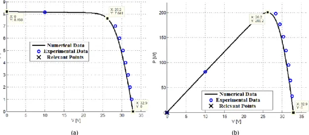
Figures 7 and 8 show the final curves I-V and P-V adjusted by the iterative method of their PV modules, which are those that most closely match to the experimental curves shown in their datasheets. The curves superpose exactly with the three most important experimental points provided by the manufacturers: Isc, Pmax,m and Voc. The main parameters obtained numerically are shown in Table 2.

(a) (b)

Figure 7 –(a) I-V and (b) P-V final curves of the PV module FV KC200GT and the three remarkable points (Isc, Pmax,m,

(8)

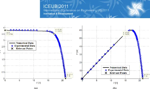
a) (b)

Figure 8 – (a) I-V and (b) P-V final curves of the PV module MSX60 and the three remarkable points (Isc, Pmax,m, Voc).

Table 2: Parameters obtained numerically for the modules FV KC200GT and MSX60 at the STC conditions.

Technical specifications Imp,e Vmp,e Imp,m Vmp,m Pmax,m Isc Voc Is1,n = Is2,n Ipv a2 Rsh Rs

Units A V A V W A V A A Ω Ω

KC200GT 7,61 26,3 7,64 26,2 200,20 8,21 32,9 4,128x10-10_{8,21 1,12 179,6 0,32} MSX60 3,5 17,1 3,51 17,1 59,86 3,80 21,1 4,704x10-10_{3,80 1,12 184,6 0,36} The resistance values calculated and the error between the experimental maximum power and the maximum power obtained numerically are shown in Table 3. Compared with the figures presented in the table, there is a good approximation of values and consequently a very small error, which shows the accuracy of the simulation program.

4. Analysis of Numerical and Experimental Curves

For a final analysis of the numerical program was necessary to compare their results with the experimental voltage and current data of the PV modules KC200GT and MSX60. Using the experimental data provided by [10-11], are drawn in Figures 9 and 10 the characteristics curves, I-V and P-V, of which module that supply a comparison between experimental and numerical values calculated using the double exponential model.

(a) (b)

(9)

(a) (b)

Figure 10 – (a) I-V and (b) P-V curves of the double exponential model and the experimental points for the PV module MSX60.

Table 3 shows the error between the experimental and numerical maximum power and the calculated relative error between curves, evaluating thus the proximity of each numerical value obtained iteratively and its experimental value of each value.

Table 3: Best values of series and shunt resistances obtained numerically for both panels and the corresponding errors between powers and between curves.

PV Model Rs [Ω] Rsh [Ω] Relative Error (Pmax) [%] Absolute Error (curves) [A]

KC200GT 0,32 179,6 0,021 0,5

MSX60 0,36 184,6 0,014 0,07

KC200GT [1-3] 0,32 160,5 - -

MSX60 [1-3] 0,35 176,4 - -

5. Conclusion

This work proposes the modeling of photovoltaic modules in MATLAB based on the double exponential model. In order for the modeling provide consistent results, it was necessary to refer to datasheets of photovoltaic modules and simulate some specific parameters. The computational modeling tool has the ability to simulate the most important features of any photovoltaic panel. The accuracy of this simulator is verified in two ways. First, when determining the best values for Rs and Rsh, the error between the experimental and numerical maximum power is very low for both panels tested. The second error verification was the comparison of experimental and numerical values of I-V and P-V characteristic curves, where there was also a low error too.

This article provides a formulation intended for numerical simulation with high accuracy performance of photovoltaic panels.

6. References

(1) Ishaque, K., Salam, Z., Taheri, H.: "Accurate MATLAB Simulink PV system simulator based on a two-diode model", Journal of Power Electronics, Vol. 11, n.º 2 (2011), pp.179-187. (2) Ishaque, K., Salam, Z., Taheri, H.: "Simple, fast and accurate two-diode model for photovoltaic modules", Solar Energy Mat. & Solar Cells, Vol. 95, n.º 2 (2011), pp. 586-594.

(10)

INTERNATIONAL CONFERENCE ON ENGINEERING UBI2011 - 28-30 Nov 2011 – University of Beira Interior – Covilhã, Portugal (3) Ishaque, K., Salam, Z., Taheri, H., Syafaruddin: "Modeling and simulation of photovoltaic (PV) system during partial shading based on a two-diode model'", Simulation Modelling Practice and Theory, Vol. 19, n.º 7 (2011), pp. 1613-1626.

(4) González-Longatt, F.M.: "Model of photovoltaic module in MatlabTM_{", 2DO Congreso} Iberoamericano de Estudiantes de Ingeniería Eléctrica (2005), Electrónica Y Computación (II Cibelec).

(5) Oi, A.: "Design and Simulation of Photovoltaic Water Pumping System", Doctoral thesis, Faculty of California Polytechnic State University, San Luis Obispo (2005).

(6) El Shahat, A.: "PV cell module modeling & ann simulation for smart grid applications", Journal of Theoretical and Applied Information Technology, Mechatronics-Green Energy Lab., Elect. & Comp. Eng., OSU, USA (2010), pp. 9-20.

(7) Walker, G.: "Evaluating MPPT converter topologies using a matlab PV model", Journal of Electrical & Electronics Engineering, Vol. 21, nº. 1 (2001), pp. 49-56.

(8) Hernanz, R., Campayo Martín, JA., Zamora Belver, J.J., Larrañaga Lesaka, I., Zulueta Guerrero, J., Puelles Pérez, E.: "Modelling of photovoltaic module'', International Conference on Renewable Energies and Power Quality (ICREPQ’10), Granada (Spain) (2010).

(9) Castañer, L., Silvestre, S.: "Modelling photovoltaic systems using PSpice", John Wiley & Sons Ltd., (2002).

(10) Villalva, M.G., Gazoli, J.R., Ruppert F., E.: "Modeling and circuit-based simulation of photovoltaic arrays", Brazilian J of Power Electronics, Vol. 14, nº.1 (2009), pp. 35-45.

(11) Villalva, M.G., Gazoli, J.R., Ruppert F., E.: "Comprehensive approach to modeling and simulation of photovoltaic arrays", IEEE Transactions on Power Electronics, Vol. 24, n.º 5 (2009), pp. 1198--1208.

(12) Gow, J.A., Manning, C.D.: "Development of a photovoltaic array model for use in power-electronics simulation studies", IEEE Proc. Elect. Power Appl., vol.146, n.º 2 (1999), pp. 193-200.

(13) Saloux, E. Teyssedou, A., Sorin, M.: "Explicit model of photovoltaic panels to determine voltages and currents at the maximum power point", Solar Energy, Vol. 85, n.º 5 (2011), pp. 713-722.

(14) Carrero, C., Rodríguez, J., Ramírez, D., Platero, C.: "Simple estimation of PV modules loss resistances for low error modelling", Ren. Energy, Vol. 35, n.º 5 (2010), pp.1103-1108. (15) Carrero, C., Rodríguez, J., Ramírez, D., Platero, C.: "Accurate and fast convergence method for parameter estimation of PV generators based on three main points of the I-V curve", Renewable Energy, Vol. 36, n.º 11 (2011), pp. 2972-2977.

(16) Chan, D.S.H., Phang, J.C.H.: “Analytical methods for the extraction of solar-cell single- and double-diode model parameters from I-V characteristics”, IEEE Transactions on Electron Devices, Vol. ED-34, n.º 2 (1987).

(17) Tsai, H.-L., Tu, C.-S., Su, Y.-J.: “Development of generalized photovoltaic model using Matlab/Simulink”, Proceedings of the World Congress on Engineering and Computer Science (2008).