CINTAL - Centro de Investiga¸
c˜
ao Tecnol´
ogica do Algarve
Universidade do Algarve
Acoustic Oceanographic Buoy Test
during the MREA’03 Sea Trial
S.M. Jesus, A. Silva and C. Soares
Rep 04/03 - SiPLAB 10/Nov/2003
University of Algarve tel: +351-289800131 Campus da Penha fax: +351-289864258
Work requested by CINTAL
Universidade do Algarve, Campus da Penha, 8000 Faro, Portugal
tel: +351-289800131, cintal@ualg.pt, www.ualg.pt/cintal Laboratory performing SiPLAB - Signal Processing Laboratory
the work Universidade do Algarve, FCT, Campus de Gambelas, 8000 Faro, Portugal
tel: +351-289800949, info@siplab.uceh.ualg.pt, www.ualg.pt/siplab
Projects LOCAPASS - FUP MdN, AOB - REA JRP
Title Acoustic Oceanographic Buoy Test during the MREA’03 Sea Trial
Authors S.M.Jesus, A.Silva and C.Soares
Date November 10, 2003
Reference 04/03 - SiPLAB Number of pages 38 (thirty eight)
Abstract This report describes the data acquired with the
Acoustic Oceanographic Buoy (AOB) during the MREA’03 sea trial, that took place aboard the R/V ALLIANCE from 18-26 June 2003, north of Elba I., Italy.
Clearance level UNCLASSIFIED
Distribution list FUP/MDN(1), SACLANTCEN (1+DVD), ULB (1+DVD), RNLNC(1), SiPLAB(1+DVD), CINTAL (1)
Total number of copies 6 (six)
III
Foreword and Acknowledgment
This report presents the AOB system and the results obtained during its testing in the MREA’03 sea trial. The MREA’03 sea trial took place off the Italian coast, near Elba I. in the period 26 May - 27 June 2003.
The authors of this report would like to thank:
• the SACLANT Undersea Research Centre for the opportunity for participating in the sea trial
• the scientist in charge Dr. Emanuel Coelho • the collaboration of Saclantcen personnel • the master and crew of the R/V Alliance
• the contribution of Prof. J.-P. Hermand from ULB for the discussions and pictures shown in this report.
IV
Contents
List of Figures VII
1 Introduction 11
2 The Acoustic Oceanographic Buoy 13
2.1 AOB hardware . . . 13
2.2 AOB software . . . 17
3 The MREA’03 sea trial 18 3.1 Generalities and sea trial area . . . 18
3.2 Ground truth measurements . . . 18
3.3 Deployment geometries . . . 19
3.4 Environmental model . . . 20
4 Acoustic data results 23 4.1 Emitted signals . . . 23
4.1.1 Emitted signals for Acoustic REA . . . 24
4.1.2 Emitted signals for underwater communications . . . 24
4.2 Received signals . . . 26
4.2.1 Received signals for acoustic REA . . . 26
4.2.2 Received signals for underwater communications . . . 26
4.3 Water column inversion . . . 27
4.3.1 The objective function . . . 27
4.3.2 Acoustic tomography results . . . 28
4.3.3 Source localization . . . 31
4.4 Underwater communications . . . 33 5 Conclusions and future developments 34
VI CONTENTS
List of Figures
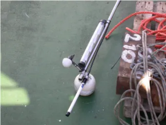
2.1 Acoustic Oceanographic Buoy - version 0: block scheme. . . 13 2.2 Acoustic Oceanographic Buoy (AOB): picture during preliminary swiming
pool testing (a) and internal configuration (b). . . 14 2.3 Acoustic Oceanographic Buoy mast: GPS cone antenna, wireless lan monopole
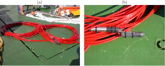
and radar reflector (long transparent tube below the antennas). . . 15 2.4 Acoustic Oceanographic Buoy (AOB): top cover (a) and bottom cover (b). . 15 2.5 Acoustic Oceanographic Buoy battery pack. . . 16 2.6 Acoustic Oceanographic Buoy (AOB): hydrophone array (a) and pre-amplifier
hydrophone package (b). . . 16
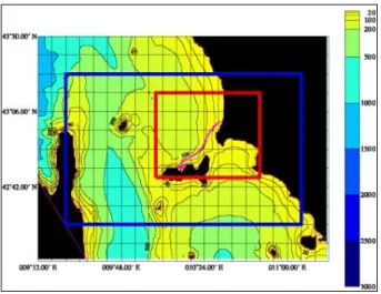
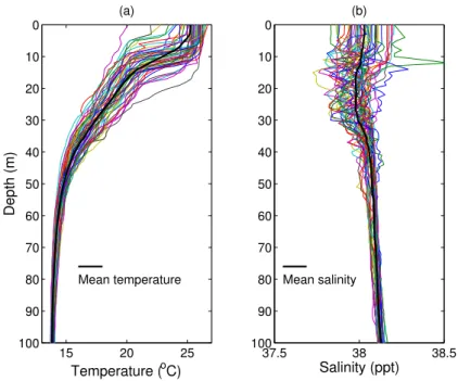
3.1 Maritime Rapid Environmental Assessment 2003 area : the channel work-ing box (blue) and the Elba workwork-ing box (red). . . 18 3.2 Recorded CTD profiles during days 16 to 19 June: temperature (a) and
salinity (b). Mean profiles are shown in thick black solid line. . . 19 3.3 Deployment of the AO-Buoy from the R/V ALLIANCE on June 21st
dur-ing the MREA’03 sea trial, off the west coast of Italy, north of Elba I. . . . 19 3.4 GPS estimated AOB and source ship navigation during the deployment of
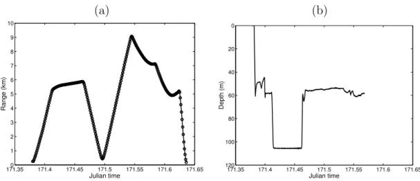
June 21 (a) and June 23 (b), 2003. . . 20 3.5 Source range (a) and depth (b) measured during AOB deployment of June
21st. . . . 21
3.6 Baseline model for the MREA’03 experiment. All model parameters are range independent except water depth. . . 21 3.7 Empirical Orthogonal Functions obtained from historical CTD data. . . 22 4.1 Transmitting source frequency response. . . 23 4.2 Transmitted LFM signals: lower band 400–900 Hz (a) and upper band 900–
1300 Hz (b). . . 24 4.3 pulse shape: root-root raised cosine (a) and its spectrum (b), root-raised
cosine (c) and its spectrum (d); continous line is for 500 symbols/s while the dashed line is for 1000 symbols/s. . . 25
VIII LIST OF FIGURES
4.4 spectograms of the transmitted signals: four distinct codes with the same total duration of 1 second of probe signal and 16 seconds of data and then 2 seconds of no signal (blue stripes), giving a total duration of 19 s for each
code. Codes are in order A, B, C and D, from left ro right. . . 26
4.5 AOB received signals during day June 21, 2003. . . 27
4.6 AOB received signals during day June 23, 2003. . . 27
4.7 AOB received code A during day June 23, 2003. . . 28
4.8 Acoustic inversion for ocean temperature during day June 21st, with signals in the band: (a) 500-800 Hz; (b) 900-1200 Hz. . . 30
4.9 Simulated data with the baseline model: α1-α2 error ambiguity surfaces in the frequency bands 500-800 Hz (a) and in 900-1200 Hz (b). . . 30
4.10 Simulated data with the baseline model in presence of 300 m source range mismatch: α1-α2 error ambiguity surfaces in the frequency bands 500-800 Hz (a) and 900-1200 Hz (b). . . 31
4.11 Noise spectrum estimated with acoustic data taken at the shallowest hy-drophone: periodogram (a) and cross-frequency power spectrum (b). . . 32
4.12 Source location using the estimated environmental parameters: source range (a) source depth (b). . . 32
4.13 virtual time reversing of the received code B for hydrophones 1, 2 and 3 (a) and summation of the time reversed data of hydrophones 1, 2 and 3 [upper plot of (b)] and detail of the probe signal pulse shape [lower plot of (b)]. . . 33
Abstract
Environmental inversion of acoustic signals for bottom and water column properties is being proposed in the literature as an interesting concept for complementing direct hydro-graphic and oceanohydro-graphic measurements for Rapid Environmental Assessment (REA). The acoustic contribution to REA can be cast as the result of the inversion of ocean acoustic properties to be assimilated into ocean circulation models specifically tailored and calibrated to the scale of the area under observation. Traditional ocean tomogra-phy systems and methods for their requirements of long and well populated receiving arrays and precise knowledge of the source/receiver geometries are not well adapted to operational Acoustic REA (AREA).
An innovative concept that responds to the operational requirements of AREA is be-ing proposed under a Saclantcen JRP jointly submitted by the the Universit´e Libre de Bruxelles (ULB), SiPLAB/CINTAL at University of Algarve, the Instituto Hidrogr´afico (IH) and the Royal Netherlands Naval College (RNLNC) and approved by Saclantcen in 2003 under the 2004 SPOW. That concept includes the development of water column and geo-acoustic inversion methods being able to retrieve environmental true properties from signals received on a drifting network of Acoustic-Oceanographic Buoys (AOB). A prototype of an AOB and a preliminary version of the inversion code, was tested at sea during the Maritime Rapid Environment Assessment’2003 sea trial (MREA’03) and is described in this report together with the results obtained.
10 LIST OF FIGURES
Chapter 1
Introduction
Environmental inversion of acoustic signals for bottom and water column properties is being proposed in the literature as an interesting concept for complementing direct hy-drographic and oceanographic measurements for Rapid Environmental Assessment (REA) [1, 2]. The acoustic contribution to REA can be cast as the result of the inversion of ocean acoustic properties to be assimilated into ocean circulation models specifically tailored and calibrated to the scale of the area under observation. REA is generally targeted to coastal areas, where detailed information is required both in time and space, which in turn, re-quires a significant acoustic coverage with several emitters and/or receivers scattered over a significant area. Traditional ocean tomography systems and methods for their requirements of long and well populated receiving arrays and precise knowledge of the source/receiver geometries are not well adapted to operational Acoustic REA (AREA).
An innovative concept that responds to the operational requirements of AREA is be-ing proposed under a 3-year duration Saclantcen Joint Research Project (JRP) jointly proposed by SiPLAB/CINTAL at University of Algarve (UALg - Portugal), by the Uni-versit´e Libre de Bruxelles (ULB - Belgium), by the Instituto Hidrogr´afico (IH - Portugal) and by the Royal Netherlands Naval College (RNLNC - The Netherlands). That JRP was approved by Saclantcen in 2002 under the 2004 SPOW. The proposed concept in-cludes the development of water column and geo-acoustic inversion methods being able to retrieve environmental true properties from signals received on a drifting network of Acoustic-Oceanographic Buoys (AOB).
In a different context, SiPLAB/CINTAL was contracted by FUP/MDN1 to develop an
easy-sea-going system and methods for passive source localization using Matched-Field Processing (MFP), under the LOCAPASS project2. That system was under development at SiPLAB/CINTAL during one year from mid 2002 to June 2003. Due to close re-quirements from these two projects LOCAPASS and AOB-JRP it was decided to build a system that could be used for the purpose of LOCAPASS project and that could continue to be used without any or with slight modifications under the AOB-JRP in the period 2004-2006.
The Maritime Rapid Environment Assessment’2003 sea trial (MREA’03) took place from May 26 to June 27, 2003, in the Ligurian Sea, with target areas at North and South of Elba Island. The sea trial involved the R/V Alliance and R/V Leonardo and the
1under the programme ”The ocean and its margins” of the Foundation of Portuguese Universities
(FUP) finnanced by the Portuguese Ministery of Defence (MDN)
12 CHAPTER 1. INTRODUCTION
scientists in charge were Emanuel Coelho and Edoardo Bovio (AUV operations). During the last period of the sea trial (18 - 27 June) a SiPLAB/CINTAL team was embarked on board the R/V Alliance, to proceed with the testing of an AOB protoype and a preliminary version of the inversion code to complement REA measurements performed by other teams. The AOB was deployed twice during that period, on June 21st and 23rd, on a free drifting configuration while the Alliance was towing a sound source and emitting coded signals in various frequency bands for acoustic inversion testing. During the second deployment, the sound source emitted also PSK signals in the 3 kHz band for communication testing.
This report is organized as follows: chapter 2 gives an overall description of the hard-ware and softhard-ware used in the AOB; chapter 3 describes the MREA’03 sea trial frame, ground truth measurements and deployment geometries; chapter 4 shows the acoustic data received on the AOB and the results obtained; finally, conclusions and future devel-opments are drawn in chapter 5.
Chapter 2
The Acoustic Oceanographic Buoy
2.1
AOB hardware
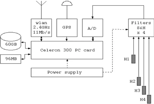
The AOB is a light acoustic receiving device that incorporates last generation technology for acquiring, storing and processing acoustic and non-acoustic signals received in various channels along a vertical line array. The physical characteristics of the AOB, in terms of size, weight and autonomy, will tend to those of a standard sonobuoy, with however the capability of local data storage, processing and online transmission. Data transmission is ensured by seamless integration into a wireless lan network, which allows for network tomography within ranges up to 10/20 kms. In this first AOB prototype there were only four acoustic channels spanning a total aperture of 90 m. The system bandwidth reaches 15 kHz which allows its usage in other applications, such as, active sonar and underwater communications. A simplified schematic is shown on figure 2.1 A photo and a detailed
Figure 2.1: Acoustic Oceanographic Buoy - version 0: block scheme.
schematic are shown in figure 2.2. The AOB photo shows the AOB cylindrical stainless steel body with top and bottom covers, during a preliminary testing on a swiming pool.
14 CHAPTER 2. THE ACOUSTIC OCEANOGRAPHIC BUOY
The red cable holds a test hydrophone that was not used during the sea trial. The antenna mast is attached to the top box cover and the bottom cover is protected by a stainless steel frame. In the schematic it can be seen the internal arrangement of the AOB (from top to bottom): the top cover with mast attachment and water tight connectors, the wireless lan amplifier, the computer box, hard disks, DC/DC converter power supply, ON/OFF switch circuitry, signal conditioning and cable buffering circuits and the battery pack. The antena mast is shown in greater detail in picture 2.3, where a 8 dBi monopole
(a) (b) PVC Computer Box WLAN AMP. hard disk DC/DC converter signal conditioning board Hyd Sensors 70 mm 350 mm 60 mm 80 mm 200 mm 210 mm Mast WLAN Cabel respire screw strength 60mm batteries Gland Gland Bulkhead cnnection AIR/Thermic insulation 170 mm 30mm 30mm 0mm 270mm 60mm 440mm 640mm 720mm 780mm 1140mm 1200mm 1260mm ON/OFF timer GPS cabel Ethernet connection Rubbery ON/OFF switch Recharge battery
connector cnnectionBulkhead
Figure 2.2: Acoustic Oceanographic Buoy (AOB): picture during preliminary swiming pool testing (a) and internal configuration (b).
antenna can be seen attached to the top mast close to the GPS cone antenna and above the linear radar reflector. Detailed pictures of the top and bottom covers are shown on figure 2.4, (a) and (b), respectively. The top cover has a number of water tight connectors, some protected by stainless steel caps. These are: the large yellow passthrough for the wireless lan antenna LR400 coaxial cable, the small passthrough for the GPS antenna RG58 coaxial cable, the large cap on the left for connecting the battery charger and the smaller cap on the right for connecting the ethernet cable to the internal computer. The idea is that when the buoy is recovered after operation these caps can be removed and the connectors accessed for battery charging and integral data retrieving from the hard disks without opening the main buoy container. The buoy stays on the deck and can be deployed next day with minimum intervention and keeping a high degree of operationality. The bottom cover clearly shows the four hydrophone connectors and in the center a water sensor for the ON/OFF automatic switch. A commmon problem when operating delicate electronic equipment from a ship is the severe deck and crane bangging suffered by the
2.1. AOB HARDWARE 15
Figure 2.3: Acoustic Oceanographic Buoy mast: GPS cone antenna, wireless lan monopole and radar reflector (long transparent tube below the antennas).
equipment during deployment. This is particularly severe for the safety of the equipment when there are moving electronic parts such as multi board computers and hard disks. One solution to avoid major damage is to deploy the system switched off, which poses the problem of how to switch it back on while at sea. That was solved in an elegant manner in the AOB by introducing a timer circuit activated by the short circuit between the water sensor on the bottom cover and the AOB main body. With this system the AOB was faultlessly activated approximately 2.5 minutes after deployment keeping intact all the electronic parts and hard disks. The hydrophone connectors and the bottom cover was protected by a stainless steel frame attached to the AOB main body and supporting also the hydrophone array cable and the ballast. The AOB computer was based on a single
(a) (b)
Figure 2.4: Acoustic Oceanographic Buoy (AOB): top cover (a) and bottom cover (b). board robust PC implementation of a Celeron 400 MHz with 256 MB RAM, a 96 MB chip disk with the operating system, output connectors for 10/100 Mb/s ethernet, USB, serial and parallel ports and video, mouse and keyboard connectors for monitoring and setup. A PCI/ISA (PISA) architecture was adopted so as to accommodate three other boards: the GPS board for precise 1 µs precision timing and localization of the buoy, a high speed 16 bit ADC board for the acoustic channels and a PCI interface for the wireless
16 CHAPTER 2. THE ACOUSTIC OCEANOGRAPHIC BUOY
interconnected in such a way as to provide 24 volts and an autonomy greater than 8 hours. The battery pack is shown on photo 2.5 during swimming pool testing. The hydrophone
Figure 2.5: Acoustic Oceanographic Buoy battery pack.
cable independently holded the four hydrophones at nominal depths of 15, 60, 75 and 90 m. A 25 kg ballast was located at the array bottom end so as to maintain the array as much close to the vertical as possible. Detailed pictures of the array cable on the R/V Alliance deck ready for deployment and an hydrophone pre-amplifier package are shown in figure 2.6(a) and (b), respectively. During the MREA’03 the AOB was deployed at two
(a) (b)
Figure 2.6: Acoustic Oceanographic Buoy (AOB): hydrophone array (a) and pre-amplifier hydrophone package (b).
occasions, during several hours, on a free drifting configuration. Source/receiver geometry was estimated from the on the buoy GPS, that served also to precisely time mark the data files being acquired. On-line processing was made possible by wireless transfer of the data and inversion in a complex range-dependent environment.
2.2. AOB SOFTWARE 17
2.2
AOB software
An important item to be tested during the MREA’03 sea trial was the AOB computer code to online control, monitor and invert the data collected with the AOB. In this preliminary test the software was separated in two parts: the sonobuoy control and monitoring and the on-line data inversion. The sonobuoy control and monitoring was performed by a specially developed Windows OS oriented program running on a laptop. This computer was fitted with a PCMCIA wireless card attached to the outdoor antenna installed on the main mast of the Alliance. During the sea trial only the omnidirectional 12 dBi antenna was used with a 1 W amplifier. This computer code was performing two main tasks: one was to get the GPS location of the buoy and follow its drift relative to the ship’s position and the test area bathymetry. The second task was to monitor the data being acquired via a specialized program interacting with the buoy PC via Windows message passing protocol, over the wireless network. With this code it was possible to view the status of the acquisition, observe and listen to the acoustic signals being acquired in selected channels, access the status of the remote computer in terms of wirelesslan link status, battery charge, hard disk space, etc... It was also possible to transfer acoustic data via ftp for on board online inversion. That data was shared on the network to a multiprocessor host devoted to data inversion. To carry out the data inversion in nearly real-time, a Dual AMD 2000+@1.667 GHz CPU rackmount computer running Linux operating system was used. The main goal was to be able to start data inversion as soon as the acoustic data was downloaded via ftp from the AOB.
The inversion software was based on code previously developed for Blind Ocean Acous-tic Tomography (BOAT) [3, 4] with different settings for the parameter search bounds and genetic algorithms (GA) conversion parameters taking into account that source po-sition was approximately known and that only very few (4) hydrophones were available. It should be remarked that BOAT aims at the inversion of ocean properties but also at the passive localization of the acoustic source so, to some extent, the aims of AREA and LOCAPASS project were simultaneously fulfiled. Towards online inversion it is crucial to previously setup the processor parameters. This was done via simulation work at the laboratory prior to embark. These simulations allowed for example to remark the extreme ambiguity of the search space when using a very sparse array with only 4 hydrophones and simultaneously searching for the source position and water column temperature. That ambiguity could be partially controlled by using tight bounds on the source-receiver ge-ometry and it was also found that higher frequency could in principle allow for a higher descrimination on the parameter space. Other settings included the adjusting of GA parameters such as mutation and cross-over probabilities, number of generations and in-dividuals, in order to allow a fair convergence to the maximum of the cost function within an acceptable computation time. This part of the work is generally done on a trial and error basis, and will not be described here. The choice of the cost function was also an important step that is described in larger detail in section 4.3.1.
On board a few steps are carried out before data inversion can start. Bathymetry data and relative source-receiver location were introduced as preliminary online informa-tion. A computer model of the environment was built based on the segmentation of the bathymetric information along the source-receiver cross sections at different times. This information together with array and source geometry (depth) are all stored in a data base together with the Empirical Orthogonal Functions (EOF) for the given data set. Now received acoustic signals can be segmented from the raw data and used for inver-sion processing. Auxiliary plots of spectograms and pulse-compressed arrival patterns are
Chapter 3
The MREA’03 sea trial
3.1
Generalities and sea trial area
The selected area for the MREA’03 is shown in the map of figure 3.1. The area covered during the acoustic operation of the AOB was included on the North Elba area (red box). During the week of June 18 and June 26, the weather was very calm with sea state between 0 and 1. Low wind of less than 2 knot from variable direction and wave height less than 1 m.
Figure 3.1: Maritime Rapid Environmental Assessment 2003 area : the channel working box (blue) and the Elba working box (red).
3.2
Ground truth measurements
Extensive ground truth measurements were performed before, during and after the tar-get week, including CTD, XBT, vessel mounted ADCP, one SEPTR buoy, two bottom mounted ADCP’s, two thermistor chains, one meteo buoy and one wave buoy. In general most of this information, except for the bottom mounted ADCP’s and thermistor chains, was recorded on board or on land stations and transmitted to onboard ship, assimilated
3.3. DEPLOYMENT GEOMETRIES 19 15 20 25 0 10 20 30 40 50 60 70 80 90 100 (a) Temperature (oC) Depth (m) Mean temperature 37.5 38 38.5 0 10 20 30 40 50 60 70 80 90 100 (b) Salinity (ppt) Mean salinity
Figure 3.2: Recorded CTD profiles during days 16 to 19 June: temperature (a) and salinity (b). Mean profiles are shown in thick black solid line.
and displayed for usage on web displays. For its relevance to the problem at hand with the acoustic data, the CTD’s collected during the week of interest are shown in figure 3.2, temperature (a) and salinity (b).
3.3
Deployment geometries
Figure 3.3: Deployment of the AO-Buoy from the R/V ALLIANCE on June 21st during the MREA’03 sea trial, off the west coast of Italy, north of Elba I.
20 CHAPTER 3. THE MREA’03 SEA TRIAL
on June 21. GPS recordings made during the deployment allowed to draw both the AOB drifting and the Alliance navigation as shown in figure 3.4 on June 21st (a) and on June 23rd (b). The June 21st AOB deployment was primarely devoted to the engineering test of
(a) (b)
Figure 3.4: GPS estimated AOB and source ship navigation during the deployment of June 21 (a) and June 23 (b), 2003.
the AOB itself, since this was the first deployment ever. The objective of the acquired data was twofold: 1) to allow source localization using a single buoy with a few hydrophones in an unknown and range-dependent environment and 2) to perform tomographic inversions for the environmental parameters and therefore serve as input to the MREA experiment. The deployment of the AOB ocurred at 11:00 local time in a relatively flat bottom area north of Elba I. and was recovered at about 17:15, as shown in figure 3.4(a). Source -receiver range varied from 500 m up to 9 km on a variable water depth area. The second deployment was devoted to test another capability of the AO-Buoy that is the ability to receive high-frequency signals used in underwater communications (UCom). On June 23rd, the deployment of the AOB ocurred at 08:30 local time in a relatively flat bottom area north of Elba I. and was recovered at about 14:00, as shown in figure 3.4(b). The sea was slightly rougher than during the deployment of June 21, with a wave height of 1 to 1.5 m. Source - receiver range varied from 500 m up to 3 km. Source depth was permanently recorded on board the R/V ALLIANCE, between 60 and 70 m depth.
The plots of figure 3.4 were also used to extract the approximate bathymetric profiles for the source-receiver transects at all times. Source depth as recorded on the source depth sensor and source range estimated from GPS are shown on figure 3.5.
3.4
Environmental model
One of the most time demanding task, and with largest impact in the final result, is the choice of an adequate environmental model to represent the propagation conditions of the experiment. This choice is generally the result of a compromise between a detailed, accurate and parameter full model and a light model ensuring a rapid convergence during the processing. The baseline model adopted for the MREA’03 was drawn from previous experiments in the area [5]. The environmental model is generally formed by a, so-called, baseline model giving a background fixed description of the propagation environment and a set of variable parameters or functions to account for spatial and time variability as well
3.4. ENVIRONMENTAL MODEL 21 (a) (b) 171.350 171.4 171.45 171.5 171.55 171.6 171.65 1 2 3 4 5 6 7 8 9 10 Julian time Range (km) 171.35 171.4 171.45 171.5 171.55 171.6 171.65 0 20 40 60 80 100 120 Julian time Depth (m)
Figure 3.5: Source range (a) and depth (b) measured during AOB deployment of June 21st.
as modelling errors. The baseline model consisted of an ocean layer overlying a sediment
0 60 120 Depth (m) Range (km) Source (60 m) Subbottom 0 3 6.0 1510 1540 m/s α=0.11 dB/λ ρ=1.82 g/cm3 1571 m/s VA Sediment 3.7 m 1477 m/s ρα=0.09 dB/λ =2.3 g/cm3 140
Figure 3.6: Baseline model for the MREA’03 experiment. All model parameters are range independent except water depth.
layer and a bottom half space with the bathymetry assumed to be range-dependent, as shown in figure 3.6. For the purposes of the inversion the forward model was divided into two parameter subsets: geometric parameters and water column temperature parameters. The baseline sediment and bottom properties were those estimated in [5] (see table 3.1). Water column variability was characterized thanks to the CTD data acquired during the previous days as shown in figure 3.2. This data was used to compute the set of Empirical Orthogonal Functions (EOF) for representing the time and space variability of the oscillations of the water column according to
ˆ T (z) = ¯T + N X i=1 αiUi(z), 0 ≤ z ≤ H (3.1)
where αi are the EOF coefficients to be estimated, Ui(z) the EOF’s and H is the water
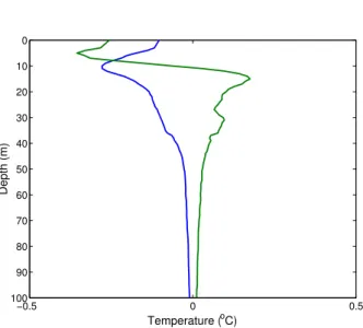
depth. The two first EOF’s are shown on figure 3.7 and they are meant to represent at least 80% of the total energy in the water column. Forward modelling was computed
22 CHAPTER 3. THE MREA’03 SEA TRIAL
Model parameter Geometric
array aperture (m) 75 sensor depth (m) 90 array tilt (rad) 0 waterdepth (m) 120 - 140 Sediment comp. speed (m/s) 1477 density (g/cm3) 2.3 attenuation (dB/λ) 0.09 thickness (m) 3.7 Bottom comp. speed (m/s) 1571 density (g/cm3) 1.82 attenuation (dB/λ) 0.11
Table 3.1: Geometric and geoacoustic parameters used in the baseline model with their respective search interval.
−0.5 0 0.5 0 10 20 30 40 50 60 70 80 90 100 Temperature (oC) Depth (m)
Chapter 4
Acoustic data results
4.1
Emitted signals
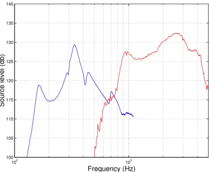
Acoustic signals were emitted from R/V Alliance with a sound source composed of two transducers, for low and high frequency bands, mounted on a single two body. The low frequency transducer was a HX90G (SN51) covering the band 180-600 Hz, while the high-frequency tansducer was an ITC2010 (SN508) roughly covering the band 700-5000 Hz. The transducers were driven by a Instruments Inc. power amplifier. Source level curves are shown in figure 4.1.
102 103 100 105 110 115 120 125 130 135 140 Frequency (Hz) Source level (db)
24 CHAPTER 4. ACOUSTIC DATA RESULTS
4.1.1
Emitted signals for Acoustic REA
The transmitted signals for AREA were linear frequency modulated (LFM) sequences in two frequency bands as shown in figure 4.2.
(a) (b)
Figure 4.2: Transmitted LFM signals: lower band 400–900 Hz (a) and upper band 900– 1300 Hz (b).
4.1.2
Emitted signals for underwater communications
The signals being transmitted with the acoustic sound source during the deployment of June 23, were computer generated time series of Phase Shift Keying (PSK) modulated binary sequences at various rates and frequency bands. A list of the transmitted codes characteristics is given in table 4.1. Each code is formed by a short time duration probe signal followed by a data packet. Probe signals and data codes are described below.
Code Probe signal Data code
Type1 Band2 Duration Type3 Band Bit rate Duration
(Hz) (second) (Hz) (bps) (second) A rrrc 1000 1 PSK2 1000 500 16 B rrrc 1000 1 PSK4 1000 1000 16 C rrrc 2000 1 PSK2 2000 1000 16 D rrrc 2000 1 PSK4 2000 2000 16
Table 4.1: characteristic parameters of the underwater communication code signals trans-mitted during June 23, 2003 [1rrrc=root-root raised cosine pulse shape, 2with 100% roll-off, 3PSK = Phase Shift Keying].
The probe signal
The probe signal acts as an header of the message itself and has always a fixed duration of 1 second. The shape of the probe signal is the pulse shape of the PSK modulation, which mainlobe duration depends on the symbol rate: the higher the symbol rate the shorter
4.1. EMITTED SIGNALS 25
the mainlobe. The pulse shape itself is a root-root raised cosine with 100% roll-off as shown in figure 4.3(a) with its spectrum shown in 4.3(b) for symbol rates of 500 and 1000 symbols/s (continous and dashed line, respectively). Figure 4.3 also shows in (c) and (d), the root-raised cosine and its spectrum, respectively. The root-root raised cosine is the actual pulse shape being transmitted, while the single root raised cosine is the pulse shape obtained at the matched-filter output, i.e., after phase conjugation and multiplication in the frequency domain.
(a) (c) 0.49 0.492 0.494 0.496 0.498 0.5 0.502 0.504 0.506 0.508 0.51 0 0.02 0.04 0.06 0.08 0.1 0.12 0.14 0.16 t [sec] (a) Pulse Shape 0.49 0.492 0.494 0.496 0.498 0.5 0.502 0.504 0.506 0.508 0 0.1 0.2 0.3 0.4 0.5 0.6 0.7 0.8 0.9 1 t [sec] (a) Raised Cossine (b) (d) −1500 −1000 −500 0 500 1000 1500 0 0.5 1 1.5 2 2.5 f [Hz] (b)
Pulse Shape Fourier Transform
−1500 −1000 −500 0 500 1000 1500 0 5 10 15 20 25 30 35 40 f [Hz] (b)
Raised Cossine Fourier Transform
Figure 4.3: pulse shape: root-root raised cosine (a) and its spectrum (b), root-raised cosine (c) and its spectrum (d); continous line is for 500 symbols/s while the dashed line is for 1000 symbols/s.
Data codes
Data codes are formed by a probe signal (PS) followed by a PSK modulated binary data sequence(DS). The binary DS is a stream of 0’s and 1’s with duration of 16 seconds at symbol rates of 500 or 1000 symb/s. The DS is formed as a random sequence of symbols that is different for each code. PSK modulations used are binary (PSK2) and quadrature (PSK4), therefore the base bit/rate is doubled for PSK4. Carrier frequency is 2.5 kHz and bandwidth’s are variable depending on symbol rate. The transducer frequency response around 2.5 kHz shows a relatively wide bandwidth reaching 1.5 kHz with an attenuation smaller than 3 dB, thus two bandwiths were used: 1000 and 2000 Hz. Data codes characteristics are summarized in table 4.1. Transmitted signals are shown in
26 CHAPTER 4. ACOUSTIC DATA RESULTS
Figure 4.4: spectograms of the transmitted signals: four distinct codes with the same total duration of 1 second of probe signal and 16 seconds of data and then 2 seconds of no signal (blue stripes), giving a total duration of 19 s for each code. Codes are in order A, B, C and D, from left ro right.
4.2
Received signals
4.2.1
Received signals for acoustic REA
An example of a spectogram of the signals received on the four hydrophones during day June 21, is shown in figure 4.5. The signals seen in this figure are a repetition of the lower band LFM’s of figure 4.2(a), that were transmitted in sequence as an attempt to increase the amount of signal energy at each frequency bin in a given time window. There are two remarks that can be made when observing this figure: one is that the data is extremely clean without blanks or interruptions; another is that there is an obvious channel fadding effect that drastically reduces the signal received on the top most hydrophone, probably due to the effect of the thermocline.
4.2.2
Received signals for underwater communications
An example of a spectogram of the signals received on the four hydrophones during day June 23, is shown in figure 4.6. Since emitter and receiver were not synchronized the codes in this figure are in the order B-C-D-A. It can be seen that the noise level on the deepest hydrophone is so high that the signals are barely perceptible. The same channel fading effect that could be seen during day June 21, is also present here, where the signal present in hydrophone number one is highly attenuated due to the strong thermocline at 30/40 m depth.
4.3. WATER COLUMN INVERSION 27
Figure 4.5: AOB received signals during day June 21, 2003.
Figure 4.6: AOB received signals during day June 23, 2003.
signal can be seen before the data is transmitted. The short probe signal duration makes it difficult to see in a spectogram due to the necessary Fast Fourier Transform time integration period.
4.3
Water column inversion
4.3.1
The objective function
28 CHAPTER 4. ACOUSTIC DATA RESULTS
Figure 4.7: AOB received code A during day June 23, 2003. model
Y(θ0) = [YT(θ0, ω1), YT(θ0, ω2), · · · , YT(θ0, ωK)]T
= H(θ0)S + U (4.1)
where Y(θ0) is the observed data vector at all hydrophones and at all discrete frequencies
in the band, H(θ0) represents the acoustic channel transfer function assumed time
invari-ant during T , with T ≤ 1/2N fmax and fmax is the maximum frequency in the signal of
interest, S is the source emitted signal spectrum and U is an additive noise term assumed to be zero mean and white. The broadband cross-frequency matched-field processor is then given by
P (θ) = tr{PHCY YPHCY Y} tr{PHCY Y}
, (4.2)
where PH = H(θ)[HH(θ)H(θ)]−1HH(θ) is a projection matrix, and where
ˆ CY Y(θ0) = 1 N N X n=1 Yn(θ0)YnH(θ0) (4.3)
is the sample correlation matrix computed with N snapshots. The Y(θ0, ωk), k = 1, ..., K
are normalized before carrying out the averaging of the outer product, and ˆCY Y(θ0) has
also norm 1. It was previously shown that this processor has identical performance than the coherent matched phase processor [8] and is well suited for low signal-to-noise ratio situations with high ambiguity and large frequency bandwidth.
4.3.2
Acoustic tomography results
Acoustic inversion was attempted on the data collected on June 21st on both frequency
bands transmitted. The time elapsed between pings was 10 minutes (between 09:54 and 11:44) for the lower frequency band, and 20 minutes (between 12:14 and 13:54) for the higher frequency band. In the processing, the sampled signals were decimated to 2.008 kHz and 4.016 kHz, for the low and high frequency bands, respectively while 22
4.3. WATER COLUMN INVERSION 29
Model parameter Lower bound Upper bound Quantization steps Geometric Source range (km) Rs - 0.3 Rs + 0.3 128 Source depth (m) Zs - 3 Zs + 3 16 Receiver depth (m) 85 95 64 Tilt (rad) -0.045 0.045 64 Watercolumn α1 (oC) -15 15 128 α2 (oC) -15 15 128
Table 4.2: Inversion of acoustic data on day June 21st: GA forward model parameters, search bounds and quantization steps. Search intervals for source range and depth are centered on the GPS estimated values.
equispaced frequency bins were taken in each band. To compute the sample correlation matrices 10 snapshots were considered. The time intervals between pings and number of frequencies were chosen such that the inversions could be achieved in due time. Due to some troubleshooting with the inversion software, the inversions could start only during the evening of June 23rd. It took about 4 days to carry out 12 inversions in the lower
frequency band and 6 inversions in the higher frequency band. This was particularly long due to the large frequency band being considered and the range dependency of the environment.
Table 4.2 shows the search parameters, their respective intervals and quantization steps when optimizing with the GA. Note that the search interval for source range and depth is always centered in the true GPS values and the bounds are relatively tight so as to allow only the slight adjustment of possible position measurement errors. The number of generations was set to 50 with 190 individuals and 3 independent populations. The muta-tion and cross-over probabilities were respectively set to 0.0056 and 0.9. The populamuta-tions were initiated using the previously estimated parameter vector: 30% of the individuals are initialized in an interval centered on the previous estimate with a search amplitude which is 10% of the total interval. The estimated temperature profiles are shown in figure 4.8. It can be seen that the temperature profiles obtained in the lower frequency band show high variability resulting in unlikely estimates through time (figure 4.8(a)). The temperature estimates at zero depth are between 21 and 30 oC, which is very unlikely
even if both time and space dependance is taken into account. On the other hand the variability of the estimates obtained on the higher frequency band (figure 4.8(b)) is clearly lower, where the temperatures at zero depth vary within more reasonable bounds of 23 to 26.5oC1.
In order to try to understand the challenge posed by the problem of estimating two EOF coefficients on an uncertain environment and how does that challenge vary with the considered frequency band, a short simulation was performed. In that simulation the baseline model of figure 3.6 was considered with the acoustic source located at 6 km range and 60 m depth and a water depth of 120 m. The synthetic data is noiseless and all cross-frequency terms have the same weight. Figure 4.9 shows the α1-α2 ambiguity surfaces
for the lower (a) and higher frequency (b) bands, respectively. The generally assumed behaviour that ambiguity decreases with frequency is not verified in this case. In fact, the result obtained in the higher frequency band (b) has a more pronounced diagonal than that in the lower frequency band (a). However, in practice there is always some degree of uncertainty in the environment and mismatch situations always occur. If, for
30 CHAPTER 4. ACOUSTIC DATA RESULTS (a) (b) 14 16 18 20 22 24 26 28 30 10 20 30 40 50 60 70 80 90 100 110 Temperature (oC) Depth (m) 14 16 18 20 22 24 26 28 30 10 20 30 40 50 60 70 80 90 100 110 Temperature (oC) Depth (m)
Figure 4.8: Acoustic inversion for ocean temperature during day June 21st, with signals in the band: (a) 500-800 Hz; (b) 900-1200 Hz.
(a) (b)
Figure 4.9: Simulated data with the baseline model: α1-α2 error ambiguity surfaces in the
4.3. WATER COLUMN INVERSION 31
(a) (b)
Figure 4.10: Simulated data with the baseline model in presence of 300 m source range mismatch: α1-α2 error ambiguity surfaces in the frequency bands 500-800 Hz (a) and
900-1200 Hz (b).
example, a source range mismatch of 300 m is encountered, the relative performance in the two bands may be altered. Figure 4.10 shows the ambiguity surfaces for estimating the EOF coefficients for the lower frequency band (a) and higher frequency band (b). It is interesting to verify that in both cases the surface maxima are now shifted towards higher values of α1. These pictures also reveal that the relative surface ambiguity has
changed: compared to the previous no-mismatch case, the lower frequency band is now more degradated than that obtained in the higher frequency band (closely spaced high level sidelobes and a spread of the main lobe). From this test it appears that the high frequency band is more robust to source range mismatches.
Another important factor that distinguishes the two frequency bands is the noise level. In terms of sidelobes, white noise would have the unharmfful effect of adding a constant to the surface, while correlated noise would desiquilibrate the main peak to sidelobe ratio, deviating the main peak to an unpredictable location. Figure 4.11 shows a noise spectrum estimate (a) and the cross-frequency spectrum (b), using analog-to-digital converted raw data. The noise was observed during 80 s at the shallowest hydrophone. Then an averaged periodogram was computed by dividing the whole observed noise signal into windows of 0.5 s, giving 160 snapshots. In plot (a) it can be seen that the estimated noise level falls off more than 15 dB in the band from 500 to 1200 Hz, showing a slight hyperbolic arch. This estimate seems to be roughly in agreement with the noise spectrum Venz curves from Urick [9], but with a slighter higher attenuation. Plot (b) shows the corresponding cross-spectrum which gives a better idea of noise cross-correlation extent being used in the cross-frequency processor. In this plot (b) each FFT is normalized. To avoid the noise power dependence and to have better estimation of the noise frequency cross-correlation the element ij of the matrix CN N can be divided by
q
CN N(ωi)CN N(ωj), which results
in a matrix with all ones in the diagonal. Plot (b) clearly shows that the degree of decorrelation increases with frequency which could eventually determine the performance that can be attained on one or on the the other frequency band.
4.3.3
Source localization
32 CHAPTER 4. ACOUSTIC DATA RESULTS (a) (b) 500 600 700 800 900 1000 1100 1200 285 290 295 300 Frequency (Hz) Power (dB)
Figure 4.11: Noise spectrum estimated with acoustic data taken at the shallowest hy-drophone: periodogram (a) and cross-frequency power spectrum (b).
(a) (b) 171.42 171.44 171.46 171.48 171.5 171.52 171.54 171.56 1 2 3 4 5 6 7 8 9 10 JulianTime Range (km) 171.42 171.44 171.46 171.48 171.5 171.52 171.54 171.56 10 20 30 40 50 60 70 80 90 100 110 JulianTime Depth (km)
Figure 4.12: Source location using the estimated environmental parameters: source range (a) source depth (b).
correct measurement errors or to compensate for mild model mismatch. This corresponds to artificially restrict the possibility of mislocating the acoustic source. Under these cir-cumstances it becomes uncertain whether a certain model estimate is in agreement with the reality. An environmental model test can be recast in the form of a range-depth source localization problem. Source location parameters are leading parameters in the sense that they work as main attractors during the GA search process. Conversely, if the environmental model is not correctly estimated, than the source cannot be correctly located during a localization search. Figure 4.12 shows the source location estimates using the previously estimated model parameters, tilt, hydrophone depth and EOF coefficients. The asterisks indicate the estimates obtained with the tight boundaries during environ-mental inversion, the circles are the range-depth estimates obtained in the lower frequency band, and the squares are those obtained in the higher frequency band. It can be seen that several estimates are incorrect. Severe errors in the estimated source location were obtained for the lower frequency band, where 5 out of 12 estimates are mislocated. For the higher frequency band the quality of the range-depth estimation is significantly better with only one severe estimation error. In principle this test should allow environmental models estimates to be discarded (as per de BOAT principle). However, in this case it appears that model mismatches can not always be associated with source-localization
4.4. UNDERWATER COMMUNICATIONS 33
errors. In the present case the main-to-sidelobe ratio is so weak that a small mismatch or noise can potentially change the position of the maximum. On the other hand, the example shown in figure 4.9 suggests that at a low SNR several pairs (α1, α2) can have a
similar MF response.
4.4
Underwater communications
During June 23, 2003 a series of communication codes were transmitted to probe the underwater acoustic channel capabilities for data communication. The scope of the pro-cessing is to use the virtual time reversal concept as presented in [10, 11]. Very simply speaking, the idea is to use the received probe signal as an image of the signal pulse shape convolved with the channel impulse response to matched-filter the received data sequence that follows the probe signal. In doing this, there is the hope that the acous-tic channel is sufficiently stable to hold during the data sequence duration, which is 16 seconds in our case. Figure 4.13(a) shows the module of the baseband signal recovered from the matched-filtering (virtual time reversing) of the data sequence of code B, for hy-drophones 1, 2 and 3. It can be seen that for all three hyhy-drophones the pulse shape peak is clearly extracted with a much better reconstruction of the data following data packet with hydrophones 2 and 3 than with hydrophone 1, due to the low signal to noise ratio. Figure 4.13(b) shows the coherent summation of the signals of plots (a). The theoretical
(a) (b) 0 0.5 1 1.5 2 2.5 0 0.5 1 1.5 2x 10 5 Hyd #1 0 0.5 1 1.5 2 2.5 0 5 10 15x 10 6 Hyd #2 0 0.5 1 1.5 2 2.5 0 5 10 15x 10 6 Hyd #3 Time 0 0.5 1 1.5 2 2.5 3 0 0.5 1 1.5 2x 10 7 ps + signal 0.5 0.505 0.51 0.515 0.52 0.525 0.53 0.535 0.54 0.545 0 0.5 1 1.5 2x 10 7 ps Time
Figure 4.13: virtual time reversing of the received code B for hydrophones 1, 2 and 3 (a) and summation of the time reversed data of hydrophones 1, 2 and 3 [upper plot of (b)] and detail of the probe signal pulse shape [lower plot of (b)].
result would be a bandbased pulse shape as a perfect raised cosine. It can be seen, by comparing with the raised cosine pulse shape of figure 4.3(c), that the pulse shape main peak is clearly extracted. This is a remarkable results taking into account the low number of hydrophones which give a very short array aperture compared to the water column. With this aperture the normal mode orthogonality condition is seldom verified resulting in a poor multipath arrival cancelation in the extracted data code. Four hydrophones, in practice reduced to three, are generally insufficient to perform virtual time reversal at
Chapter 5
Conclusions and future developments
As a remote sensing tool, shallow water acoustic inversion, can bring valuable information to traditional REA. Acoustic REA is therefore an area of considerable interest for which adapted systems and methods are required. The AOB Saclantcen JRP aims at developing and testing a new integrated methodology that includes, in its final stage, the airborne deployment of a random network of specialized sonobuoys and online acoustic inversion algorithms for estimating water column and sea bottom properties. As a preliminary step towards that aim, an AOB prototype and an initial set of inversion algorithms was tested during the MREA’03 sea trial. That included two deployments of the AOB, during which the concept of a light, yet fully operational, acoustic buoy was proved successful. Full online positioning, data monitoring and transfer was possible up to a range of approxi-mately 9 km. The online inversion was started during the deployment but first inversion results where only available at the end of the cruise.
When evaluating the results, there are two mais aspects to be considered: one is techni-cal and regards the AOB hardware development and setup and the other is scientific and is related to the inversion algorithm and its integration with the hardware system. On the hardware point of view, this test indicated that the concept is feasible, i.e., a small and light system can be developed to acquire, process, store and transmit acoustic and oceanographic data for REA purposes. The embedded PC technology and its wireless lan philosophy is to be pursued. The size and weight of the buoy can be reduced and the number of acoustic and oceanographic channels can and should be increased. The on-the-buoy processing capabilities can be used for data reduction and pre-processing for monitoring. On the online acoustic inversion side it was shown that it is indeed possible to invert acoustic data from a free drifting operational buoy. However, it was also shown that the number of existing acoustic channels (four in the actual version) is clearly not sufficient for a reliable water column inversion. This number needs to be at least dou-bled in the near future. It was also shown that, at least with four acoustic channels, a frequency band centered in 1 kHz provided more robust and reliable results than a lower band around 500 Hz. The online inversion code also needs a better interfacing with the data acquisition and monitoring software.
As a side note it should be referred that the AOB hardware prototype was developed with the contribution of the FUP/MDN finnanced LOCAPASS project, that was termi-nated in June 2003, and which aimed at passive source localization. In fact it was also shown with the REA acoustic data, that source localization could be seen as a by prod-uct of the acoustic inversion if the array was well populated and with known geometry [3, 4] or as an environmental consistency checking scheme if the environmental model was
35
assumed known. Thus the data acquired during the MREA’03 has also shown that it is possible to localize a sound source with a sparse free-drifting vertical array of acoustic sensors if the environment is reasonably well known.
Besides the theoretical aspect, this project was marked by an important technological advance: an acoustic receiving portable buoy was developed in a Portuguese institution - the AOB. Although, each component of the AOB is not new or highly sophisticated, it is the assembling concept and the multipurpose character of the system, seen as a whole, that represents a technological breakthrough. Its main innovative characteristics are: i) the AO-Buoy is a portable system, easy to deploy and recover from a small ship, or from a workboat (airplane or helicopter in a future version), ii) it features an inboard programable computer that allows for receiving, storing, monitoring and transmitting different types of signals and for different applications ranging from sonar detection, localization, tomog-raphy, rapid environmental assessment (REA) and underwater communications (UCom), iii) the combined capabilities of the AO-Buoy GPS and wireless lan allow for easy position tracking and time synchronization, a must for tomography, and finnaly iv) the AO-Buoy wireless lan provides a mean for easy networking into future tomography networks and/or REA systems. Moreover it is the integration between this hardware tool and the respec-tive software scientific applications that makes this system unique. SiPLAB and CINTAL are working hard to develop the follow up of the present version of the AOB into a full featured 8 hydrophone array, with enclosed temperature sensors and real time applica-tions for tomographic inversion. The next deadline is scheduled for March/April 2004 during another Saclantcen sea trial foreseen to take place off the south coast of Portugal (gulf of Cadiz/Algarve).
Bibliography
[1] Elisseeff P., Schmidt H., and Xu W. Ocean acoustic tomography as a data assimila-tion problem. IEEE Journal of Oceanic Engineering, 27(2):275–282, 2002.
[2] Lermusieux P.F.J. and Chiu C.-S. Four-dimensional data assimilation for coupled physical-acoustical fields. In Pace and Jensen, editors, Impact of Littoral Environment Variability on Acoustic Predictions and Sonar Performance, pages 417–424, Kluwer, September 2002.
[3] Jesus S.M., Soares C., Onofre J., and Picco P. Blind ocean acoustic tomography: Experimental results on the intifante’00 data set. In Proc. Sixth of European Conf. on Underwater Acoust., ECUA’02, Gdansk, Poland, June 2002.
[4] Jesus S.M., Soares C., Onofre J., Coelho E., and Picco P. Experimental testing of the blind ocean acoustic tomography concept. In Pace and Jensen, editors, Impact of Littoral Environment Variability on Acoustic Predictions and Sonar Performance, pages 433–440, Kluwer, September 2002.
[5] Soares C., Waldhorst A., and Jesus S. Matched field processing: Environmental focusing and source tracking with application to the north elba data set. In Proc. of the Oceans’99 MTS/IEEE conference, pages 1598–1602, Seattle, Washington, 13-16 September 1999.
[6] Ferla C.M., Porter M.B., and Jensen F.B. C-SNAP: Coupled SACLANTCEN normal mode propagation loss model. La Spezia, Italy.
[7] Soares C. and Jesus S.M. Broadband matched-field processing: coherent vs. incoher-ent approaches. J. Acoust. Soc. America, 113(5):2587–2598, May 2003.
[8] Orris G.J., Nicholas M., and Perkins J.S. The matched-phase coherent multi-frequency matched field processor. J. Acoust. Soc. America, 107:2563–2575, 2000. [9] Urick R.J. Principles of Underwater Sound. McGraw-Hill, New York, 1983.
[10] Silva A., Jesus S., Gomes J., and Barroso V. Underwater acoustic communica-tions using a “virtual” electronic time-reversal mirror approach. In P. Chevret and M.Zakharia, editors, 5th European Conference on Underwater Acoustics, pages 531– 536, Lyon, France, June, 2000.
[11] Jesus S.M. and Silva A. Virtual time reversal in underwater acoustic communications: Results on the intifante’00 sea trial. In Proc. of Forum Acusticum, Sevilla, Spain, September 2002.
Appendix A
MREA’03 DVD-ROM list
The acoustic data gathered with the Acoustic-Oceanographic buoy as well as file logs and auxiliary reading files are contained in two DVD-ROMs, attached to the back cover of this report. Tables A.1 e A.2 list and describes all DVD-ROM files and directories.
Table A.1: DVD ROM June 21, 2003 reference: MREA03-01-SiPLAB
Dir name sub-dir Content Time(start-end) AcousticData A2double array data1 09:01:20-09:38:40
A1 array data 09:40:00-11:54:40 A2 array data 12:05:20-14:01:19 A1double array data 14:07:59-14:43:59 DirectPath ref. hydrophone @1m2
Noise array data - noise only Auxiliary EmittedSignal computer generated emitted
signals (mat files - 16bits) Log log of acoustic emissions Software data reading m-files
NonAcousticData Bathymetry bathymetry files of the area CTD ctd files of June 21
Navigation ship and source naviation SourceDepth source depth readings Jun 21
1 low power emmissions to warn possible marine mammals in the area 2 only a single chirp for each code signal.
38 APPENDIX A. MREA’03 DVD-ROM LIST
Table A.2: DVD ROM June 23, 2003 reference: MREA03-02-SiPLAB Dir name sub-dir Content Time(start-end) AcousticData PSK array data 06:54:19-11:38:34
Noise array data - noise only Auxiliary EmittedSignal computer generated emitted
signals (mat files - 16bits) Log log of acoustic emissions Software data reading m-files
NonAcousticData Bathymetry bathymetry files of the area CTD ctd files of June 21
Navigation ship and source naviation SourceDepth source depth readings Jun 23