Frequency-Domain Receiver Design for Doubly-Selective Channels

(1)

Mestre

Frequency-Domain Receiver Design for

Doubly-Selective Channels

Dissertação para obtenção do Grau de Doutor em Engenharia Electrotécnica e de Computadores

Orientador :

Prof. Dr., Rui Dinis, FCT-UNL

Co-orientador :

Prof. Dr., Paulo Montezuma, FCT-UNL

Júri:

Presidente: Prof. Dr. Paulo Pinto, FCT-UNL Arguentes: Prof. Dr. Paulo Silva, ISE-UALG

Prof. Dr. Francisco Cercas, ISCTE-IUL Vogais: Prof. Dr. Paulo Montezuma, FCT-UNL

(2)

(3)

Frequency-Domain Receiver Design for Doubly-Selective Channels

Copyright cFábio José Pinto da Silva, Faculdade de Ciências e Tecnologia, Univer-sidade Nova de Lisboa

The Faculdade de Ciências e Tecnologia and the Universidade Nova de Lisboa have the perpetual right, without geographical limits, to archive and publish this disserta-tion either in print or digital form, or any other medium that is still to be invented, and distribute it through scientific repositories, admitting its copy and distribution for ed-ucational or research purposes, as well as for non-commercial purposes, as long as the author and the editor are credited for their work.

(4)

(5)

Your love taught me to be hopeful and courageous without fear and frustration.

(6)

(7)

(8)

(9)

Abstract

This work is devoted to the broadband wireless transmission techniques, which are se-rious candidates to be implemented in future broadband wireless and cellular systems, aiming at providing high and reliable data transmission and concomitantly high mobility. In order to cope with doubly-selective channels, receiver structures based on OFDM and SC-FDE block transmission techniques, are proposed, which allow cost-effective im-plementations, using FFT-based signal processing.

The first subject to be addressed is the impact of the number of multipath compo-nents, and the diversity order, on the asymptotic performance of OFDM and SC-FDE, in uncoded and for different channel coding schemes. The obtained results show that the number of relevant separable multipath components is a key element that influences the performance of OFDM and SC-FDE schemes.

Then, the improved estimation and detection performance of OFDM-based broad-casting systems, is introduced employing SFN (Single Frequency Network) operation. An initial coarse channel is obtained with resort to low-power training sequences estima-tion, and an iterative receiver with joint detection and channel estimation is presented. The achieved results have shown very good performance, close to that with perfect chan-nel estimation.

The next topic is related to SFN systems, devoting special attention to time-distortion effects inherent to these networks. Typically, the SFN broadcast wireless systems employ OFDM schemes to cope with severely time-dispersive channels. However, frequency er-rors, due to CFO, compromises the orthogonality between subcarriers. As an alternative approach, the possibility of using SC-FDE schemes (characterized by reduced envelope fluctuations and higher robustness to carrier frequency errors) is evaluated, and a tech-nique, employing joint CFO estimation and compensation over the severe time-distortion effects, is proposed.

(10)

direction of travel. This represents a severe impairment in wireless digital communica-tions systems, since that multipath propagation combined with the Doppler effects, lead to drastic and unpredictable fluctuations of the envelope of the received signal, severely affecting the detection performance. The channel variations due this effect are very dif-ficult to estimate and compensate. In this work we propose a set of SC-FDE iterative ceivers implementing efficient estimation and tracking techniques. The performance re-sults show that the proposed receivers have very good performance, even in the presence of significant Doppler spread between the different groups of multipath components.

(11)

Resumo

Nos últimos anos tem-se vindo a assistir a um rápido desenvolvimento de técnicas de transmissão de banda larga sem fios, sendo capazes de fornecer ritmos de transmissão elevados, mesmo em cenários de elevada mobilidade. De modo a lidar com sistemas duplamente seletivos, é dado neste trabalho especial ênfase à concepção de estruturas de recepção adequadas a cenários caracterizados por canais fortemente dispersivos no tempo e na frequência. Para tal, são usadas técnicas de transmissão por blocos assistidas por prefixos cíclicos (CP), permitindo assim que essas técnicas sejam implementadas, a baixo custo, através do processamento de sinal baseado na transformada de Fourier discreta, FFT (Fast Fourier Transform).

Numa primeira fase foi abordado o impacto do número de componentes multiper-curso, assim como da ordem de diversidade, no desempenho assimptótico de esquemas OFDM e SC-FDE, em cenários sem codificação de canal, ou usando diferentes tipos de codificação de canal. Os resultados obtidos mostram que o número de componentes multipercurso é um factor chave que influencia o desempenho de esquemas OFDM e SC-FDE.

O tema seguinte tem como foco as redes de frequência única, SFN (Single Frequency Network), e apresentada um método com vista ao melhoramento do desempenho da es-timação e deteção conjunta de sistemas de difusão baseados em OFDM. Inicialmente é obtida uma estimativa do canal com recurso a sequências de treino de baixa potência. Essa estimação é posteriormente melhorada com recurso a um recetor iterativo Decision-Directed, onde é realizada estimação e deteção conjunta. Os resultados alcançados

indi-cam um desempenho muito bom, perto do desempenho obtido com estimação perfeita do canal.

(12)

de envolvente, assim como uma maior robustez a erros da frequência da portadora), e proposta uma nova técnica que, com recurso à estimação e compensação conjunta das rotações de fase, permite obter resultados de desempenho muito satisfatórios.

Por último, são considerados sistemas de transmissão em banda larga sem fios, em cenários onde movimento relativo entre emissor e recetor induz um desvio de Doppler diferente para cada componente multipercurso (por sua vez dependente do ângulo de incidência desse raio em relação à direção do deslocamento). Quando combinada com efeitos de Doppler, a propagação multipercurso conduz a flutuações drásticas e imprevi-siveis da envolvente do sinal recebido, levando a variações de canal extremamente difí-ceis de estimar e compensar. Como tal, surgem muitas dificuldades ao nível da deteção e, consequentemente, levando à degradação do desempenho deste tipo de sistemas. Neste trabalho são propostos recetores iterativos para o SC-FDE, implementando técnicas efici-entes de estimação e seguimento das variações do canal. Os resultados de desempenho mostram que estes recetores têm muito bom desempenho, mesmo na presença de fortes desvios de Doppler.

(13)

List Of Acronyms

ADC Average Doppler Compensation

AWGN Additive White Gaussian Noise

BER Bit Error Rate

BLUE Best Linear Unbiased Estimator

CFO Carrier Frequency Offset

CP Cyclic Prefix

CIR Channel Impulse Response

CLT Central Limit Theorem

DAB Digital Audio Broadcasting

DAC Digital-to-Analog Converter

DFT Discrete Fourier Transform

DFE Decision Feedback Equalizer

DVB Digital Video Broadcasting

DVB-T Digital Video Broadcasting - Terrestrial

EIRP Effective Isotropic Radiated Power

FDE Frequency-Domain Equalization

FDM Frequency Division Multiplexing

FFT Fast Fourier Transform

(18)

IB-DFE Iterative Block-Decision Feedback Equalizer

IDFT Inverse Discrete Fourier Transform

IFFT Inverse Fast Fourier Transform

IBI Inter-Block Interference

ICI Inter-Carrier Interference

ISI Inter-Symbol Interference

LLR Log-Likelihood Ratio

LOS Line-Of-Sight

MC Multi-Carrier

MFB Matched Filter Bound

MLR Maximum Likelihood Receiver

MMSE Minimum Mean Square Error

MRC Maximal-Ratio Combining

MSE Mean Square Error

OFDM Orthogonal Frequency-Division Multiplexing

PAPR Peak-to-Average Power Ratio

PMEPR Peak-to-Mean Envelope Power Ratio

PDF Probability Density Function

PDP Power Delay Profile

PSD Power Spectral Density

PSK Phase Shift Keying

QAM Quadrature Amplitude Modulation

QPSK quadrature Phase-Shift Keying

SC Single Carrier

SC-FDE Single Carrier with Frequency Domain Equalization

SINR Signal to Interference-plus-Noise Ratio

(19)

SNR Signal to Noise Ratio

SISO Soft-In, Soft-Out

TDC Total Doppler Compensation

(20)

(21)

List Of Symbols

General Symbols

Ae effective area or “aperture” of an antenna

B bandwidth of a given frequency domain signal

BD Doppler spread

Bk feedback equalizer coefficient for thekthfrequency

BC coherence bandwidth

c speed of light (inm/s)

cl(τ, t) channel response, at timet, to a pulse applied att−τ

Eb average bit energy

Es average symbol energy

F subcarrier separation

Fk feedforward equalizer coefficient for thekthfrequency

F_k(l) feedforward equalizer coefficient for thekth_{frequency and}_lth_{diversity branch}

f frequency variable

fc carrier frequency

fD maximum Doppler frequency

f_D(r) Doppler drift associated to therthcluster of rays

fk kthfrequency

(22)

Gt gain of the transmitter antenna

Gr gain of the receiver antenna

i tap index of the diversity branch

g(t) impulse response of the transmit filter

Hk overall channel frequency response for thekthfrequency

˜

HkL overall channel frequency response estimation for thekthfrequency

H_k(l) overall channel frequency response for thekthfrequency andlthdiversity branch

H_k(m) overall channel frequency response for thekthfrequency of themthtime block

˜

HD

k data overall channel basic frequency response estimation for thekthfrequency

ˆ

H_kD data overall channel enhanced frequency response estimation for thekthfrequency

˜

H_kT S training sequence overall channel basic frequency response estimation for thekth frequency

ˆ

H_kT S training sequence overall channel enhanced frequency response estimation for the kthfrequency

˜

H_kT S,D overall channel basic frequency response combined estimation for the kth

fre-quency

ˆ

H_kT S,D overall channel enhanced frequency response combined estimation for the kth frequency

h(t) channel impulse response

hb(t) complex baseband representation ofh(t)

hT(t) pulse shaping filter

˜

hD

n data overall channel basic impulsive response estimation for thenthtime-domain

sample

ˆ

hD_n data overall channel enhanced impulsive response estimation for the nth time-domain sample

˜

hT S_n training sequence overall channel basic impulsive response estimation for thenth time-domain sample

ˆ

hT S

n training sequence overall channel enhanced impulsive response estimation for the

(23)

˜

hT S,Dn overall channel basic impulsive response combined estimation for thenth

time-domain sample

ˆ

hT S,Dn overall channel enhanced impulsive response combined estimation for the nth

time-domain sample

J0 zeroth-order Bessel function of the first kind

k frequency index

L number of paths within a multipath fading channel

Ls system losses due to hardware

LIn(i) in-phase log-likelihood ratio for thenthsymbol at theithiteration

LQn(i) quadrature log-likelihood ratio for thenthsymbol at theithiteration

l antenna index/diversity branch

m data symbol index

N number of symbols/subcarriers

N0 noise power spectral density (unilateral)

ND number of data blocks

NRx space diversity order

NT S number of symbols of the training sequence

Nk channel noise for thekthfrequency

N_kT S training sequence channel noise for thekthfrequency

N_k(l) channel noise for thekthfrequency andlthdiversity branch

N_k(m) channel noise for thekth_{frequency of the}_mth_{time block}

NG number of guard samples

n time-domain sample index

n(t) noise signal

P L meanpath-lossin dB

P L path-lossfor the free space model

Pb AWGN channel performance

(24)

Pb,Ray performance of a single ray transmitted between the transmitter and the receiver

Pe bit error rate

ˆ

Pe estimated bit error rate

Pr(d) received power as a function of the distanced

Pt transmitted power

R symbol rate

R(f) Fourier transform ofr(t)

R(τ) autocorrelation function

r(t) rectangular pulse/shaping pulse

rhbhb(t1, t2) autocorrelation function ofhb(t)

S(f) frequency-domain signal

Sk kthfrequency-domain data symbol

ST S

k training sequencekthfrequency-domain data symbol

S_k(m) kth_{frequency-domain data symbol of the}_mth_{data block}

˜

Sk estimate for thekthfrequency-domain data symbol

˜

S_k(m) estimate for thekthfrequency-domain data symbol of themthdata block

ˆ

Sk “hard decision” for thekthfrequency-domain data symbol

ˆ

S_k(m) “hard decision” for thekthfrequency-domain data symbol of themthdata block

Sk “soft decision” for thekthfrequency-domain data symbol

s(t) time-domain transmitted signal

sb(t) complex baseband representation ofs(t)

s(t)(m) _{signal associated to the}_mth_{data block}

sI₍_t₎ _{continuous in-phase component}

sQ(t) continuous quadrature component

sn nthtime-domain data symbol

sI_n discrete in-phase component

(25)

sT S_n training sequencenthsymbol

s∆ _{time-domain transmitted signal affected by carrier frequency offset}_∆

f

˜

sn sample estimate of thenthtime-domain data symbol

˜

s(nm) estimate of thenthtime-domain data symbol of themthdata block

˜

s(f_D(r)) _{sample estimate of the}_nth_{time-domain data symbol associated to the}_rth_cluster

of rays, affected by a Doppler shiftfD

ˆ

sn “hard decision” of thenthtime-domain data symbol

ˆ

s(nm) “hard decision” of thenthtime-domain data symbol of themthdata block

sn “soft decision” of thenthtime-domain data symbol

T duration of the useful part of the block

TB block duration

TCP duration of the cyclic prefix

TD duration of the data blocks

TF frame duration

TG guard period

Tm sample time

Tm delay spread

TS symbol time duration

TT S duration of the training block

Ta sampling interval

T0 fundamental period

t time variable

Ul discrete taps order for thelthdiversity branch

Utotal total of discrete taps order forNRxspace diversity order

X random number

Xσ normal (or Gaussian) distributed random variable (RV) with zero mean and

stan-dard deviationσ

(26)

Yk received sample for thekthfrequency

Y_kT S training sequencekthfrequency-domain received sample

Y_k(m) kthfrequency-domain received sample of themthdata block

Y_k(l) received sample for thekthfrequency andlthdiversity branch

yn nthtime-domain received sample

y_nT S training sequencenthtime-domain received sample

y(fD)

n nthtime-domain received sample affected by Doppler shiftfD

y(f

(r) D )

n nthtime-domain received sample associated to therthcluster of rays, affected by

Doppler shiftfD

yn(l) nthtime-domain received sample for thelthdiversity branch

y(t) received signal in the time-domain

yb(t) complex baseband representation ofy(t)

wn nthchannel noise sample

αl attenuation of given multipath component

β relation between the average power of the training sequences and the data power

∆f carrier frequency offset

∆(_ki) error term for thekthfrequency-domain “hard decision” estimate

∆(_km) zero-mean error term for thekth frequency-domain “hard decision” estimate of themth_{data block}

γ(i) average overall channel frequency response at theithiteration

κ(i) normalization constant for the FDE

λc wavelength of the carrier frequency (measured in meters)

ρ(i) correlation coefficient at theithiteration

ρm correlation coefficient of themthdata block

ρI_n correlation coefficient of the “in-phase bit of thenthdata symbol

ρQn correlation coefficient of the “quadrature bit of thenthdata symbol

(27)

σ_Eq2 total variance of the overall noise plus residual ISI

ˆ

σ2

Eq approximated value ofσEq2

σ_MSE2 mean-squared error (MSE) variance σ_N2 variance of channel noise

σ2

S variance of the transmitted frequency-domain data symbols

σ_{H,T S}2 variance of the noise in the channel estimates related with the training sequence

σ_D2 variance of the noise in the channel estimates related with the data blocks

σT total received power from the scatterers affecting the channel at given delayτ

σ_{T S,D}2 variance of the noise in the combined channel estimates

Θk overall error for thekthfrequency-domain sample

Θ(k) mean-squared error (MSE) in the time-domain

θl angle between the direction of the movement and the direction of departure of the

lthcomponent.

θn phase rotation due to CFO associated to thenthsample

θ(nr) estimated phase rotation due to Doppler frequency drift

ε(_ki) global error consisting of the residual ISI plus the channel noise at theithiteration

εEq_k (i) denotes the overall error for thekth_{frequency-domain symbol}

ϑI_n error insˆI_n

ϑQn error insˆQn

Ω2

i,l mean square value of the magnitude of each tapifor thelthdiversity branch

ωc frequency carrier (in rads/s)

Φr set of all multipath components

φ phase offset

φDop,l Doppler phase shift of thelthmultipath component

ϕi,l(t) zero-mean complex Gaussian random process

τi,l delay associated to theithtap andlthdiversity branch

(28)

νl represents AWGN samples

ǫH_kL channel estimation error

ǫD_k data channel estimation error

ǫT S_k training sequence channel estimation error

ǫT S,D_k combined training and data channel estimation error

Matrix Symbols

z Utotal×1vector

zH conjugate transpose ofz

Σ Σis aUtotal×UtotalHermitian matrix

z Utotal×1vector

Rl autocorrelation function matrix ofR(τ)associated to thelthdiversity branch

Ψ covariance matrix ofz

Λ diagonal matrix whose elements are the eigenvaluesΛi(i=1,..,Utotal) ofΣ′

(29)

List of Figures

2.1 Reflection effect. . . 10

2.2 Diffraction effect. . . 10

2.3 Scattering effect. . . 11

2.4 Multipath Power Delay Profile: Power transmitted (a); Channel impulse response (b) . . . 12

2.5 Frequency response of a certain channel and bandwidth of signal (in or-ange): Narrowband signal (a); Wideband signal (b) . . . 14

2.6 Transmission of a symbols(t)through wireless channelh(t) . . . 15

2.7 Mobile communication system . . . 15

2.8 Example of alth incident wave affected by the Doppler effect. . . 22

2.9 A mobile receiver within a multipath propagation scenario. . . 24

2.10 Tapped delay line model of a doubly-selective channel in the equivalent complex baseband. . . 25

2.11 Fast fading due to mobility: the signal strength exhibits a rapid variation with time. . . 27

2.12 Difference in path lengths from the transmitter to the mobile station. . . . 27

2.13 Example of an uniform scattering scenario . . . 28

2.14 Doppler power spectrum density . . . 29

2.15 Zeroth-order Bessel function of the first kind. . . 30

3.1 Transmission structure for multicarrier modulation. . . 34

3.2 Receiving structure for multicarrier modulation. . . 36

3.3 (a) Transmission ofN information symbols onN subcarriers in timeN/B; (b) Transmission of1information symbol in1/Btime.. . . 36

3.4 Transmission structure for multicarrier modulation with resort to the IFFT block. . . 40

(30)

3.6 MC burst’s final part repetition in the guard interval. . . 42

3.7 Basic OFDM transmission chain. . . 44

3.8 (a) Overlapping bursts due to multipath propagation; (b) IBI cancelation by implementing the cyclic prefix. . . 45

3.9 OFDM Basic FDE structure block diagram with no space diversity. . . 45

3.10 OFDM receiver structure with aNRx-branch space diversity. . . 46 3.11 Basic SC-FDE transmitter block diagram. . . 48

3.12 Basic SC-FDE receiver block diagram. . . 49

3.13 Basic SC-FDE receiver block diagram with anNRx-order space diversity. . 50 3.14 Basic transmission chain for OFDM and SC-FDE. . . 51

3.15 Performance result for uncoded OFDM and SC-FDE. . . 51

3.16 IB-DFE receiver structure (a) without diversity (b) with aNRx-branch space diversity. . . 53

3.17 Uncoded BER perfomance for an IB-DFE receiver with four iterations. . . 55

3.18 Improvements in uncoded BER perfomance accomplished by employing “soft decisions" in an IB-DFE receiver with four iterations. . . 57

3.19 SISO channel decoder soft decisions . . . 58

4.1 BER performance of an IB-DFE in the uncoded case. . . 65

4.2 RequiredEb/N0to achieveBER= 10−4for the uncoded case and without

diversity, as a function of the number of multipath components. . . 66

4.3 BER performance for a rate-1/2 code. . . 67

4.6 Required Eb/N0 to achieve BER = 10−4 for the rate-1/2 convolutional

code, as function of the number of multipath components. . . 69

4.9 RequiredEb/N0 to achieveBER = 10−4 at the MFB and at the4th

itera-tion of the IB-DFE, for an uncoded scenario without diversity and with a Nakagami channel model with factorµ. . . 70

4.10 BER performance of OFDM and SC-FDE, forU =2, 8 and 32, and a

Nak-agami channel withµ= 4. . . 71

5.1 Single frequency network transmission. . . 74

5.2 Frame structure. . . 75

5.3 Impulsive response of the channel estimation with method I. . . 78

5.4 Impulsive response of the channel estimation with method II. . . 79

(31)

5.6 Impulsive response of the channel estimation with method IV. . . 80

5.7 BER performance for OFDM withND = 1block andβ= 1/16. . . 83 5.8 BER performance for OFDM withND = 4block andβ= 1/16. . . 83 5.9 UsefulEb/N0 required to achieveBER = 10−4 withND = 1, as function

ofβ: OFDM for the4th_iteration. _{. . . .} ₈₄ 5.10 TotalEb/N0required to achieveBER= 10−4withND = 1, as function of

β: OFDM for the4thiteration. . . 85

6.1 Equivalent transmitter plus channel. . . 90

6.3 Channel estimation for thepth block of data. . . 93

6.4 Receiver structure for Method II. . . 95

6.5 Receiver structure for Method III. . . 96

6.6 BER performance for the proposed methods, with a power relation of10dBs between both transmitters, and considering values of:∆f(1)₋∆f(2) = 0.05

(a);∆f(1)₋∆f(2) = 0.1(b). . . 99

6.7 BER performance for the proposed methods, with a power relation of10dBs between both transmitters, and considering values of:∆f(1)₋∆f(2) = 0.15

(a);∆f(1)₋_∆f(2) _{= 0.175}_(b). _{. . . 100}

6.8 Method I . . . 101

6.9 Method II. . . 101

6.10 Method III . . . 102

6.11 Impact of the received power on the BER performance, with∆f(1)₋∆f(2)= 0.15, and employing the frequency offset compensation for Method II. . . 102

6.12 Impact of the received power on the BER performance, with∆f(1)₋_∆f(2)₌

0.15, and employing the frequency offset compensation for Method III. . . 103

7.1 Doppler shift. . . 106

7.2 Various objects in the environment scatter the radio signal before it arrives at the receiver (a); Model where the elementary components at a given ray have almost the same direction of arrival (b). . . 108

7.3 Jakes Power Spectral Density (a); PSD associated to the transmission of a single ray (b); PSD associated to the transmission of multiple rays (c). . . 109

7.4 Multipath components having the same direction of arrivalθare grouped into clusters. . . 110

7.6 Equivalent cluster of rays plus channel. . . 115

7.7 Receiver structure for ADC. . . 117

7.8 Receiver structure for TDC. . . 118

(32)

7.10 BER performance for a scenario with normalized Doppler drifts fd and

−fdforfd= 0.05. . . 120 7.11 BER performance for a scenario with normalized Doppler drifts fd and

−fdforfd= 0.09. . . 120

B.1 The spectrumS(f) . . . 131

B.2 The spectrumS+(f) . . . 132

(33)

1

Introduction

1.1 Motivation and Scope

The tremendous growth of mobile internet and multimedia services, accompanied by the advances in micro-electronic circuits as well as the increasing demands for high data rates and high mobility, motivated the rapid development of broadband wireless systems over the past decade. Future wireless systems are expected to be able to deploy very high data rates of services within high mobility scenarios. As a result, broadband wireless com-munication is nowadays a fundamental part of the global information and the world’s communication structure.

A major challenge in the design of mobile communications systems is to overcome the mobile radio channel effects, assuring at the same time high power and spectral effi-ciencies. Since in mobile communications the information data is transmitted across the wireless medium, then the transmitted signal will certainly suffer from adverse effects originated by two different factors: multipath fading and mobility.

Within a multipath propagation environment waves arriving from different paths with different delays combine at the receiver with different attenuations. Multipath prop-agation leads to the time dispersion of the transmitted symbol resulting in frequency-selective fading.

(34)

depending on the location of the user, and because of mobility, they also vary in time. Hence, when the relative positions of the different objects in the environment including the transmitter and receiver change with time, the nature of the channel also varies. In mobility scenarios, the rate of variation of the channel response in time is characterized by the Doppler spread. Significant variations of the channel response within the signal

duration lead totime-selective fading, and this represents a major issue in wireless

com-munication systems.

Channels whose response is selective in time and frequency are referred as doubly-selective. As a result of these two phenomena, the equivalent received signal is time varying and may be highly attenuated. This is considered a severe impairment in wire-less communication systems, since these effects lead to drastic and unpredictable fluctu-ations of the envelope of the received signal (deep fades of more than 40 dB bellow the mean value can occur several times per second).

Block transmission techniques, with cyclic extensions and FDE techniques (Frequency-Domain Equalization), are known to be suitable for high data rate transmission over severely time-dispersive channels due to its reduced complexity and excellent perfor-mance, provided that accurate channel estimates are provided. Moreover, since these techniques usually employ large blocks, the channel can even change within the block duration. Fourth generation broadband wireless systems employ CP-assisted (Cyclic Prefix) block transmission techniques, and although these techniques allow the simpli-fication of the receiver design, the length of the CP should be a small fraction of the overall block length, meaning that long blocks are susceptible to time-varying channels, especially for mobile systems. Hence, the receiver design for doubly-selective channels is of key importance, especially to reduce the relative weight of the CP.

Efficient channel estimation techniques are crucial onto achieving reliable communi-cation in wireless communicommuni-cation systems. When the channel changes within the block duration then significant performance degradation occur. Channel variations lead to two different difficulties: first, the receiver needs continuously accurate channel estimates; second, conventional receiver designs for block transmission techniques are not suitable when there are channel variations within a given block. As with any coherent receiver, accurate channel estimation is mandatory for the good performance of FDE receivers, both for OFDM (Orthogonal Frequency-Division Multiplexing) and SC-FDE (Single Car-rier with Frequency Domain Equalization).

(35)

an associated frequency offset. This leads to a very difficult scenario where there will be substantial variations on the equivalent channel which can not be treated as simple phase variations.

For channel variations due to Doppler effects, receiver structures for double-selective channels combining an iterative equalization and compensation of channel variations, have already been proposed [5]. These kind of channel variations can become extremely complex since the Doppler effects are distinct for different multipath components (e.g., when we have different departure/arrival directions relatively to the terminal move-ment).

It is difficult to ensure stationarity of the channel within the block duration, which is a requirement for conventional OFDM and SC-FDE receivers. Hence, efficient estimation and tracking procedures are required, and should be able to cope with channel variations.

1.2 Objectives

This work considers the study of effective detection of broadband wireless transmission, and it is intended for future broadband wireless and cellular systems which should be able to provide high transmission, together with high mobility (e.g., WiFi/WiMax-type LANs).

(36)

(37)

2

Fading

In order to enable communication over wireless channels it is necessary to characterize the propagation models. However, trying to make an analysis of the mobile communica-tion under such harsh propagacommunica-tion condicommunica-tions might seem a very hard task to accomplish. Nevertheless, starting from a model based on the multipath propagation we will see that many of the properties of the transmission can be successfully predicted with resort to powerful techniques of statistical communication theory [6].

One of the major challenges in the design of mobile communications systems is to overcome the effects of mobile radio channels, assuring at the same time reliable high-speed communication. Parameters like the paths taken by the multipath components, the presence of objects along these paths and the distance between the transmitter and receiver, have a direct influence on the signal.

The wireless channel experiences deep fade in time or frequency. Fading effects re-lated with mobile communications can be classified in two spatial scales:

• Large scale fading: based onpath-lossand shadowing;

• Small scale fading: based on multipath fading and Doppler spread.

2.1 Large Scale Fading

(38)

2.1.1 Path-Loss

The signal attenuation of an electromagnetic wave (represented by a reduction in its power density), between a transmitting and a receiving antenna as a function of the propagation distance, is called path-loss. As the relative distance between the

transmit-ter and receiver increases, the power radiated by the transmittransmit-ter dissipates as the radio waves propagate through the channel. This is commonly referred asfree-space path-loss

and refers to a signal propagating between the transmitter and receiver with no attenua-tion or reflecattenua-tion. This is the simplest model for signal propagaattenua-tion and is based on the free-space propagation law. Let us consider the free-space propagation model. It consid-ers the line of sight channel in which there are no objects between the receiver and the transmitter, and it attempts to predict the received signal strength assuming that power decays as a function of the distance between the transmitter and receiver.

The Friis free space equation states that for a transmission between a transmitter and receiver separated by a distanced, then the power acquired by the receiver’s antenna, as a function of thed, is given by [7],

Pr(d) =

PtGtGrλ2 (4π)2_d2_L

s

, (2.1)

where Pt stands for the transmitted power (assumed to be known in advance),Gtand

Gr represent the gains at the transmitter and receiver antenna, respectively, considering

that both antennas are isotropic. The parameterλis the wavelength measured in meters, and is related with the carrier frequency by

λ= c

fc

= c 2π/ωc

, (2.2)

withcrepresenting the speed of light (in m/s),fc representing the carrier frequency (in

Hertz),ωcthe frequency carrier (in rads/s). TheLsis a factor representing system losses

which are inherent to hardware, and not related with propagation issues (assuming that there are no losses in the system, we will consider a value ofLs= 1).

By definition, the antenna’s gain is related with the antenna’s effective area or “aper-ture” by,

G= 4πAe

λ2 , (2.3)

where the apertureAeis related with the dimensions of the antenna. However, in

wire-less systems are used isotropic antennas in order to have reference antenna gains. An isotropic radiator consists in an ideal antenna which transmits energy uniformly in all directions, having unit gain(G= 1).

It can be seen from equation (2.1) that the received power falls off with the square of the distanced, which can be quantified as a decay with distance at a rate of 20 dB/decade [7].

(39)

is measured in dB, and it gives the difference between the effective isotropic radiated power (EIRP) and the received power, and consists in a theoretical measurement of the maximum radiated power available from a transmitter in the direction of maximum an-tenna gain, as compared to an isotropic radiator. Thepath-lossfor the free space model is given by

P L= 10 log Pt

Pr

=₋10 log

GtGrλ2 (4π)2_d2

, (2.4)

It can be seen that in free-space, we have

P L_∝d2. (2.5)

However, in practical scenarios in which the transmitted signal may be reflected, the power signal decays faster with distance. Several propagation models show that the average received signal power decreases in a logarithmical form with distance. And it is defined that the average large-scale path-loss (over a infinity of different points) for

a distance dbetween the transmitter and receiver, can be given as a function ofdwith resort topath-lossfactorn, which is the rate at which thepath-lossincreases with distance.

Therefore, a simple model forpath-lossgiven by [7], may be

P L=P L(d0) + 10nlog

d d0

,[dB] (2.6)

where P L(d0) is the mean path-loss in dB at distanced0 (the bar in the equation refers to the joint average of all possible loss values). It is also important to point out that the since equation (2.1) is not defined ford= 0, then the termd0is used as a known received power reference point [7]. Hence, the received powerPr(d), at a given spatial separation

d > d0, may be related toPr(d0). This reference point can be obtained analytically with resort to equation (2.1), or experimentally by measuring the received power in several locations sited in a radial distanced0 from the transmitter, and performing the average. Typically, depending on the size of the covered area,d0is assumed to be 1 kmfor large cells and 100mfor microcells. It is that linear regression for a minimum mean-squared estimate (MMSE) fits ofP Lversus don a log-scale produce a direct line with constant decay of 10 dB/decade (which in free-space, with n = 2, results in the 20 dB/decade

slope mentioned above).

2.1.2 Shadowing

Another type of large scale fading is calledshadowing, and it is caused by obstacles (e.g.,

clusters of buildings, mountains, etc.), between the transmitter and receiver. As a result a portion of the transmitted signal is lost due to reflection, scattering, diffraction and even absorption.

It is important to note that equation (2.6), which defines thepath-lossversus distance

(40)

any particular path. Hence, as a result ofshadowing, the received power in two different locations at the same distancedfrom the transmitter, may have very different values of

path-loss than the ones predicted by equation (2.6). Since the environment of different

locations with the same distancedmay be different, it is therefore needed to introduce variations about the mean loss defined in equation (2.6).

Several measurements in real scenarios have shown that thepath-loss P Lat a given distance d is a random variable characterized by a log-normal distribution about the mean value P L [8]. Therefore the measured path-loss P L (in dB) varies around the distance-dependent mean loss (given by equation (2.6)), and thereforeLP can be writ-ten in terms ofP Lplus a random variable (R.V.),Xσ, by [7]

P L=P L(d) +Xσ =P L(d0) + 10nlog(

d d0

) +Xσ,[dB] (2.7)

where, Xσ is a normal (or Gaussian) distributed random variable (RV) with zero mean

and standard deviation σ, and this RV represents the effect of shadowing. This distri-bution is suitable to define the random effects associated with thelog-normal shadowing

phenomenon, and it considers that several different measure points at a given distanced, have a Gaussian distribution around the mean loss defined in equation (2.6) [7]. In sum, in order to statistically define the path-loss caused by large-scale fading for a given dis-tanced, a set of values have to be defined:path-lossexponent, reference pointd0, standard deviationσof the RVXσ.

2.2 Small Scale Fading

A very important type of fading normally considered in wireless communication sys-tems, is related with rapid changes in the signal’s amplitude and phase that occur over very short variations in time or in the spatial area between the receiver and the transmit-ter (in fact, drastic changes in signal strength may be noticed even in half a metransmit-ter shift). The propagation model that describes this type of fading is called small-scale fading and can be expressed by two factors [7]

• Delay spread Tm, due to the multipath propagation. It is related with frequency

selectivity which in the time domain translates in time dispersion of the signal;

• Doppler spread BD, due to relative motion between the transmit and/or receive

antenna. It is related with time selectivity which in the frequency domain translates in frequency dispersion of the signal frequency components.

Moreover, in mobile transmission the velocity also plays an importance role in the type of fading experienced by the signal.

(41)

properties of the signal and the characteristics of the channel. Depending on these char-acteristics, a set of different effects of small-scale fading can be experienced. As we will see next, while multipath delay spread leads to time dispersion and frequency selective fading, Doppler spread leads to frequency dispersion and time selective fading. The two propagation mechanisms are independent of one another. The propagation models char-acterizing these rapid fluctuations of the received signal amplitude over very short time durations are called small-scale fading models.

2.2.1 The Multipath Channel

The main difference between a wired and wireless communication system lies in the propagation environment. In a wired communication system there is only a single path propagation between the transmitter and the receiver. On the other hand, wireless com-munication can be affected by distinct natural phenomena like interference, noise and others that represent serious impairments. Since that most of mobile communication systems are used within urban environments, a major constraint is related with the fact that the mobile antenna is well bellow the height of the nearby structures (such as cars, buildings, etc.), and as a consequence, the radio channel is influenced by those struc-tures. In fact, since that within this type of scenarios the line-of-sight component does not usually exists, then communication is only possible due to the influence of propagation mechanisms (reflection, diffraction and scattering of the multipath waves). The wireless communication system is characterized by a multipath propagation environment, a phe-nomenon in which the incoming multipath components arrive at the receiving antenna by different propagation paths, giving rise to different propagation time delays and lead-ing the signal to fade. Multipath fadlead-ing may be caused by a set of effects which signifi-cantly affect signals’ propagation in wireless transmission, such as reflection, diffraction and scattering.

Reflection occurs when an electromagnetic wave encounters a surface that is large

rela-tive to the wavelength of the propagation wave (e.g., walls of a building, hills, and other large plain surfaces), and it is illustrated in Fig.2.1.

Diffraction occurs when the path between the transmitter and receiver is obstructed by

an object with large dimensions when compared to the wavelength of the propaga-tion wave, being diffracted on the edges of such objects (e.g., cars, houses, moun-tains). The wave tends to travel around the object allowing the signal to be received, even if the receiver is shadowed by the large object. It is illustrated in Fig.2.2.

Scattering occurs when incoming signal hits an object whose size is in the order of the

(42)

Transmitter Receiver Building

Figure 2.1: Reflection effect.

Receiver

Transmitter

Building

(43)

number of reflections in small objects in the mobile’s vicinity. It is illustrated in Fig.

2.3.

Transmitter

Receiver Scatterer

Figure 2.3: Scattering effect.

In a multipath propagation environment, several copies of the transmitted signal ar-riving from different paths, and having different delays, combine at the receiver with different attenuations. Furthermore, depending on the delay, each incoming signal will have different phase factor. Depending on their relative phases, these multipath com-ponents will add up constructively or destructively, causing fluctuations in the overall received signal’s amplitude. And depending on the addition of the signal copies across the received path, the receiver will see a single version of the transmitted signal with a corresponding gain (attenuation) and phase. While constructive interference affects the overall signal positively since it increases the amplitude of the overall signal, de-structive interference is caused by mutual cancelation of different multipath components leading to a decrease of the signal level. If the multipath fading channel has very long path lengths, then copies of the original signal may arrive at the receiver after one sym-bol duration, which will interfere with the detection of the posterior symsym-bol, resulting in inter-symbol interference (ISI), and thus inducing distortion which causes significant degradation of the performance of the transmission. In this case, the multipath compo-nents will no longer be separable in time. Still they can be separated in frequency, and therefore the inter-symbol interference can be compensated with resort to frequency do-main equalization. This will be seen later in the subsequent chapters.

Assume that the transmitter transmits a very short pulse over a time multipath chan-nel. Two important parameters have to be taken into account: the symbol’s time du-ration, TS, and the delay spreadTm (also known as maximum excess delay time). The

(44)

−2 0 2 4 6 8 10

x 10−6 0

0.5 1 1.5 2

Transmitted Power

Delay (s)

Magnitude

(a)

−5 0 5 10 15 20

x 10−6 0

0.5 1 1.5 2

Bandlimited impulse response

Delay (s)

Magnitude

(b)

(45)

TS is transmitted, the symbol will be spread out by the channel, and at the receiver side

its length will be theTS added with the delay spreadTm. Depending on the relation

be-tweenTSandTm, the degradation can be classified in two types: flat fading or frequency

selective fading. Basically, if the delay spread is much smaller than the symbol period then the channel exhibits flat fading and the ISI can be neglected. On the other hand, if the delay spread is equal or greater than the symbol period, the channel introduces ISI that must be compensated.

Frequency Selective Fading

The multipath channel introduces time spread in the transmitted signal, since due to multipath reflections, the channel impulse response will appear as a series of pulses, as illustrated in Fig. 2.4. The multipath components may sum construc-tively or destrucconstruc-tively, and the receiver sees an overall single copy of the transmit-ted signal, characterized by a given gain (i.e. attenuation) and phase. If the channel impulse response has a delay spreadTmgreater than the symbol periodTS of the

transmitter signal, (i.e.,Tm > TS), then the dispersion of the transmitted symbols

within the channel will lead to ISI causing distortion on the received signal.

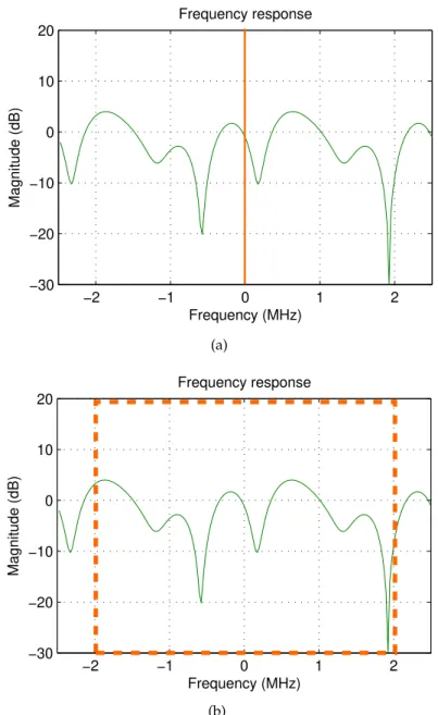
In the frequency domain, the spectrum of the received signal shows that the band-width of transmitted signal is greater than the coherence bandband-width of the channel, and in these conditions the channel induces frequency selective fading over the bandwidth. A channel parameter called coherence bandwidth,BC, is used to

char-acterize the fading type. It consists in a statistical measure of the frequency band-width in which the channel characteristics remain similar (i.e., “flat”). Essentially, signals with frequencies separated by less than BC will experience very similar

gains. Notwithstanding, a signal undergoes flat fading if in the frequency domain BS ≪ BC, and in the time domainTS ≫ Tm, as illustrated in Fig. 2.5(a). On the

other hand, if the bandwidth of the transmitted symbol is greater than the channel coherence bandwidth, BS > BC, and in the time domain Tm > TS, then

differ-ent frequency compondiffer-ents of the signal experience differdiffer-ent fading. In such con-ditions, spectrum of the received signal with different frequency components will have some components with greater gains than others. Thus, frequency-selective fading causes distortion of the transmitter signal since that the signal’s spectral components are not all affected in the same way by the channel. In fact, as it can be seen in Fig. 2.5(b) when the signal’s bandwidth is greater than the coherence bandwidth of the channel, the spectral components placed within the coherence bandwidth will be affected in a different way when compared to the components that are not covered by it. It is important to note that the coherence bandwidthBC,

and the delay spreadTm, can be related byBC = _T1_m. Thus, the coherence

(46)

−2 −1 0 1 2 −30

−20 −10 0 10 20

Frequency response

Frequency (MHz)

Magnitude (dB)

(a)

−2 −1 0 1 2

−30 −20 −10 0 10 20

Frequency response

Frequency (MHz)

Magnitude (dB)

(b)

(47)

The equivalent received signal, within a multipath scenario consists of a large number of components with randomly distributed angles of arrival, amplitudes and phases.

Modeling the Multipath Channel

We wish to model the wireless propagation channel as the system illustrated in Fig.2.6.

( )

h t

( )

s t

y t

( )

Transmitted Signal Wireless Channel Received Signal

Figure 2.6: Transmission of a symbols(t)through wireless channelh(t)

Assume that the system has an impulse response h(t), and that a transmitter sends

a signal s(t), (which in Fig. 2.6 is presented at the system’s input). Assume that s(t)

propagates through a wireless channel characterized by a responseh(t), with the output

of the signal corresponding to the received signal at the receiver. In a linear time invariant systems we have: if the signal s(t) is passed through h(t), the output y(t) will be the convolution betweens(t)andh(t). From the theory of linear systems, we know that an

attenuation is simply a scaling of the signal, which corresponds to multiplying the signal by a scaling constant denoted by attenuation factor (or gain), and is denoted byαl. On

the other hand, a delay simply corresponds to an impulse functionδ(t₋τl), whereτlis

the respective delay.

Let us look at mobile communication system illustrated in Fig. 2.7Regarding the0th

Transmitter Receiver

0 path (direct)th 1 path (scattered)st

2 path (scattered)nd

Figure 2.7: Mobile communication system

path, the signals(t)is attenuated byα0and delayed byτ0, and this can be represented as a system with impulse responseα0δ(t−τ0). In the same way, the1stpath can be described by a attenuationα1 and a delay τ1, with that corresponding path being represented by

(48)

component plusL₋1scattered components), we can model the wireless channel as a combination of all paths as

h(t) =α0δ(t−τ0) +α0δ(t−τ0) +. . .+αL−1δ(t−τL−1) =

L−1

X

l=0

αlδ(t−τl) (2.8)

and it becomes clear that the wireless channel impulse responseh(t)can be given by the

sum of the impulse responses of the Lpaths. Thus, the wireless channel can be repre-sented as a sum of multipath components each one characterized by a given attenua-tion and delay, as in Fig. 2.4. The multipath fading channel is therefore modeled as a linear finite impulse-response (FIR) filter. The channel’s filtering behavior is caused by the sum of amplitudes and delays of the multipath components at the same instant of time. The channel will behave as a filter, whose frequency response exhibits frequency selectivity. In the frequency domain, this refers to the case in which the bandwidth of the transmitted symbol is greater than the channel coherence bandwidth then the signal will suffer from frequency selective fading. Different components of the transmitted sig-nal will suffer from different attenuations and therefore will have different gains. Thus, frequency-selective fading causes the distortion of the transmitter signal since that the signal’s spectral components are not all affected in the same way by the channel. The coherence bandwidth and the delay spread are inversely related: the larger the delay spread, less is the coherence bandwidth and the channel is said to be more frequency selective.

Modeling the Transmitted Signal

Having modeled the wireless propagation channel, it is important to characterize the transmitted signals(t)through the wireless channel.

Typically the signal to be transmitted is band-limited, i.e., defined in[₋B, B]Hz and

zero elsewhere. Such signals which primarily occupy a range of frequencies centered around0Hz are called low-pass (or baseband) signals.

The majority of the wireless communication systems use modulation techniques in which the information bearing baseband signals are upconverted using a sinusoidal car-rier of frequencyfcbefore transmission, in order to move the signals away from the DC

component and center them in a appropriate frequency carrier. The resulting transmitted signals(t)will have a spectrumS(f)which is zero outside of the rangefc−B < |f|<

fc +B, wherefc >> B (i.e., the bandwidth B of the spectrum S(f) is much smaller

than the carrier frequencyfc). The term passband is often applied to these signals.

Con-sidering a communication system in which the involved signals can be measured by the received antenna (i.e., typically voltage signals), the transmitted signals and received sig-nals are typically referred as real passband sigsig-nals.

(49)

signal, located in much higher frequencies when compared with the baseband frequency. Since the information is contained in the modulated signal and not in the carrier fre-quency used for the transmission, then a model to define the signals(t) independently

of the carrier frequency fc, must be derived. The passband transmitted and received

signals, are therefore converted to the corresponding equivalent baseband signal, which is processed by the receiver in order to recover the information. Hence, a very simple representation was developed to achieve this, and is calledcomplex basebandorlow-pass equivalent representation of the communication (passband) signal, and is detailed in B.

Therefore, the signal s(t) consists on a passband signal transmitted at the carrier fre-quency, and is written as

s(t) =Rensb(t)ej2πfct o

,

where sb(t) corresponds to the complex baseband representation of s(t). The real and

imaginary parts of the complex quantity sb(t) carry information about the signal’s

in-phase and quadrature components (the components that are modulating the termscos(2πfct)

andsin(2πfct), respectively).

Modeling the Received Signal

Let us now derive the received signal at the receiver, after passing through the wireless channel. The received signaly(t)consists in a convolution of the transmitted signals(t)

with the wireless channelh(t). In order to better understand this process, let us derive

component by component. Passing the signal s(t) through the 0th _{component (LOS),}

given byα0δ(t−τ0), then the signal will be attenuated byα0and delayed byτ0. Hence, the received signal corresponding to this specific path is simply,

y0(t) =Re

n

α0sb(t−τ0)ej2πfc(t−τ0)

o

, (2.9)

In the same way, the signal corresponding to the1st component is given by

y1(t) =Re

n

α1sb(t−τ1)ej2πfc(t−τ1)

o

. (2.10)

The same procedure is repeated for the rest of the components, with the signal corre-sponding to theL₋1paths being given by

y₍_L₋₁₎(t) =Renα₍_L₋₁₎sb(t−τ(L−1))ej2πfc(t−τ(L−1))

o

. (2.11)

The overall received signal can be represented as the sum of all signal contributions, i.e.,

y(t) =Re

(_L₋₁ X

l=0

αlsb(t−τl)ej2πfc(t−τl) )

(50)

Clearly, the carrier term given byej2πfct, is common to all terms. By isolating_ej2πfctthen

(2.12) can be rewritten as

y(t) =Re

( _L₋₁ X

l=0

αlsb(t−τl)e−j2πτl !

ej2πfct )

. (2.13)

In (2.13), the term inner brackets consists in a complex baseband received signal, hence (2.13) can be rewritten as

y(t) =Renyb(t)ej2πfct o

(2.14)

where the equivalent complex baseband representation ofy(t)is

yb(t) = L−1

X

l=0

αlsb(t−τl)e−j2πτl (2.15)

and the equivalent lowpass representation of the channel is

hb(t) = L−1

X

l=0

αle−j2πτlδ(t−τl). (2.16)

The complex baseband received signal at the receiver, given byyb(t), consists in the sum

of the Lreceived multipath components, each one having a corresponding attenuation αl, and delayτl.

Let us assume that the baseband signal of different values ofτlis approximatelysb(t),

therefore, (2.13) can be simplified with resort to the narrowband assumption, since all the termssb(t−τl)are approximately equal tosb(t), this is,

yb(t) =sb(t) L−1

X

l=0

αle−j2πτl. (2.17)

and we reach to a point in which an analytical model of the wireless transmission system can be defined as

yb(t) =hb(τ)sb(t). (2.18)

Let us focus on the equivalent lowpass representation of the channel, hb(τ), where τ

corresponds to a given delay. A fundamental factor can be observed from the above ex-pression. We will call it phase factor, and it denotes the term given bye−j2πτl. It has been

explained before that since the different multipath components travel through different distances, they are received with different delays. The delay induces a phase at the sig-nal received relative to thelth multipath component, and it is clear that the phase factor e−j2πτlarises out of the delay_τ

l. As a result of the different delays, the multipath

(51)

Since that the exact knowledge of the attenuation and delay values for all of the multi-path components is impossible in real time wireless transmissions, a statistical approach can be taken in order to understand the properties of the complex fading coefficient. Hence, instead of trying to characterize each component separately, it is possible to de-scribe the properties of the equivalent lowpass representation of the channel as a whole, with resort to the theory of random processes, statistics and probability. The statistical characteristics of the channel exhibiting small-scale fading can be modeled by several probability distribution functions. Notwithstanding, considering the existence of a large number of scatterers within the channel (contributing to the received signal), and assum-ing that the different scatterers are independent, then the central limit theorem (CLT) can be used to approximate the components as independent Gaussian R.V.’s, and therefore allowing to model the channel impulse response as a Gaussian process.

Let us statistically analyze the equivalent lowpass representation of the channel, in order to draw some conclusions about its random behavior. We can apply a small mod-ification to (2.18) in order to write it as a sum of the real part and imaginary part, i.e.,

yb(t) =hb(τ)sb(t)

=sb(t) L−1

X

l=0

αle−j2πfcτl

=sb(t) L−1

X

l=0

αlcos(2πfcτl)−αlsin(2πfcτl),

(2.19)

where the real part and imaginary parts of this complex-valued quantity are given by (2.20) and (2.21), respectively,

X=

L−1

X

l=0

αlcos(2πfcτl) !

, (2.20)

Y =

L−1

X

l=0

−αlsin(2πfcτl) !

. (2.21)

HereXandY are both random numbers depending on the random quantities given by αl andτl. The randomness of this components is due to the fact that each component is

arising from the multipath environment. The wireless channel can therefore be analyzed with resort to statistical propagation models, where the channel parameters are modeled as stochastic variables. Hence,XandY are derived as the sum of a large number of ran-dom components, and in these conditions we can assume thatXandY are both Gaussian random variables. Hence,hb(τ)can be rewritten as

(52)

Considering thatXandY are Normal-distributed, then

X_∼N(0,1/2) (2.23)

Y _∼N(0,1/2) (2.24)

this is,X andY can be described as Gaussian random variables of mean zero and vari-ance1

2. Assuming that the process has zero mean, then the envelope of the received signal can be statistically described by a Rayleigh probability distribution, with the phase uni-formly distributed in(0,2π). Hence, assuming thatXandY are independent R.V.’s then the joint distribution ofXY can be expressed by the product of the individual distribu-tions ofXandY, which are given by

fX(x) = 1

√

2πσe

−(x−µ)2 2σ2

= _√1

πe−

x2

,

(2.25)

and

fY(y) = √1 2πσe

−(y−µ)2 2σ2

= _√1

πe

−y2

.

(2.26)

with the joint distribution given by

fX,Y(x, y) =fX(x)·fY(y)

= _√1

πe−

(x2₊_y2₎ (2.27)

which allows to obtain the joint distribution of the components ofhb(τ).

2.2.2 Time-Varying Channel

Besides multipath propagation, time variations within the channel may also arise due to oscillator drifts, as well as due to mobility between transmitter and receiver. Oscillator drifts consist on frequency errors relative to the frequency mismatch between the local oscillator at the transmitter and the local oscillator at the receiver and can be caused by due to phase noise or residual CFO. These channel variations lead to simple phase variations that are relatively easy to compensate at the receiver [2], [4].

Time Variation Due to Carrier Frequency Offset

(53)

order to better understand how the CFO affects the coherent detection of the transmitted signal, let us illustrate a scenario in which a transmitter sends a signals(t) that passes

through the channel and is recovered by the receiver. Assume the existence of a mismatch between the local oscillator at the transmitter and the local oscillator at the receiver, in which the transmitter sendss(t) over a carrier fc + ∆f when it should usefc. On the

receiver side, the local oscillator is tuned to the reference carrier frequencyfc. How will

this affect the received signal? Consider that the transmitted signal is given by

s(t) =Rensb(t)ej2π(fc+∆f)t o

,

withsb(t)denoting the baseband representation ofs(t). However, the receiver does is not

aware about the frequency offset at the transmitter side. Since it interprets the baseband representation ofs(t)ass∆(t) = sb(t)ej2π∆ft(when it is not), and interprets the term as

the carrier frequencyej2π(fc). The received signal will be written as

y(t) =Re

Z _∞

−∞

hb(t, τ)sb(t−τ)dτ ej2πfctej2π∆ft

=ej2π∆ft_Re

Z _∞

−∞

hb(t, τ)sb(t−τ)dτ ej2πfct

,

(2.28)

and the equivalent baseband is given by

yb(t) =ej2π∆ft Z ∞

−∞

hb(t, τ)sb(t−τ)dτ, (2.29)

which in the discrete time domain is given by

yn=ej2πθn L−1

X

l=0

hn,lsn−l, (2.30)

where the CFO is given byθn= ∆fT. Looking to the received signal in the discrete time

(54)

Time Variation Due to Movement

We have seen before that the wireless channel can be described as a function of time (and space), with the equivalent received signal resulting of the combination of the different replicas of the original signal arriving at the receiving antenna by different propagation paths, and delays. These multipath components will suffer from interference in a con-structive or decon-structive way, depending on their relative phases. As a consequence, this effect will cause fluctuations in the received signal. Now, considering that either the transmitter or the receiver is moving, this propagation phenomenon will be time vary-ing. When there is relative motion between the mobile and the fixed based station, the multipath components experiences an apparent shift in frequency, called Doppler shift (dependent on the mobile speed, carrier frequency, and the angle that its propagation vector makes with the direction of motion). Small-scale fading based on Doppler spread can be classified in fast fading or slow fading channel, depending on how rapidly the transmitted baseband signal changes as compared to the rate at which of variation of the channel.

The relative motion between the transmitter and the receiver results in Doppler fre-quency shift, leading to channel variations which are not easy to compensate. Notwith-standing, the Doppler effect has a strong negative impact on the performance of mobile radio communication systems since it causes a different frequency shift for each inci-dent plane wave. Fig. 2.46illustrates the transmission through a channel characterized by multipath propagation, between a mobile transmitter traveling with speedv, and a fixed receiver. Due to the relative movement between the transmitter and receiver, the