Faculdade de Ciências e Tecnologia
Master Dissertation
Integrated Master on Biomedical Engineering
Detection of Purkinje Images for
Automatic Positioning of Fixation
Target and Interferometric
Measurements of Anterior Eye
Chamber
Mariana Quelhas Dias Rodrigues Almeida
(student number 23279)
Faculdade de Ciências e Tecnologia
Master Dissertation
Detection of Purkinje Images for Automatic Positioning of
Fixation Target and Interferometric Measurements of
Anterior Eye Chamber
Mariana Quelhas Dias Rodrigues Almeida (student number 23279)
Adviser:
Prof. Rainer Leitgeb, Medical University of Vienna
Co-Adviser:Prof. Branislav Grajciar, Medical University of Vienna
Work presented as part of the Integrated Master on Biomed-ical Engineering, as parcial requirement for a Master de-gree in Biomedical Engineering.
To Professor Rainer Leitgeb, whose guidance and knowledge were an inspiration.
To Professor Branislav Grajciar, on whose guidance I relied and from whom I learned so much. To my parents, for their support and help along this path.
To João, for his support and inspiration.
In cataract surgery, the eye’s natural lens is removed because it has gone opaque and doesn’t allow clear vision any longer. To maintain the eye’s optical power, a new artificial lens must be inserted. Called Intraocular Lens (IOL), it needs to be modelled in order to have the correct refractive power to substitute the natural lens.
Calculating the refractive power of this substitution lens requires precise anterior eye cham-ber measurements. An interferometry equipment, the AC Master from Zeiss Meditec, AG, was in use for half a year to perform these measurements. A Low Coherence Interferometry (LCI) measurement beam is aligned with the eye’s optical axis, for precise measurements of anterior eye chamber distances. The eye follows a fixation target in order to make the visual axis align with the optical axis. Performance problems occurred, however, at this step. Therefore, there was a necessity to develop a new procedure that ensures better alignment between the eye’s visual and optical axes, allowing a more user friendly and versatile procedure, and eventually automatizing the whole process.
With this instrument, the alignment between the eye’s optical and visual axes is detected when Purkinje reflections I and III are overlapped, as the eye follows a fixation target.
In this project, image analysis is used to detect these Purkinje reflections’ positions, eventu-ally automaticeventu-ally detecting when they overlap.
Automatic detection of the third Purkinje reflection of an eye following a fixation target is possible with some restrictions. Each pair of detected third Purkinje reflections is used in automatically calculating an acceptable starting position for the fixation target, required for precise measurements of anterior eye chamber distances.
Keywords: Fixation target, Image analysis, Eye’s optical and visual axis, Low Coherence
Interferometry (LCI), Purkinje reflections, (Eye length) IOL measurements
Na cirurgia da catarata, a lente natural do olho é retirada por se ter tornado opaca e já não permitir uma visão clara. Para manter o poder óptico do olho é necessário inserir uma nova lente artificial. Esta lente, designada por Intraocular Lens - IOL (lente intraocular), em inglês, precisa de ser modelada de forma a ter o poder refractivo correcto para tomar o lugar da lente natural.
O cálculo do poder refractivo da lente de substituição requere medições precisas da câmara anterior do olho. Um instrumento de medição interferométrica, o AC Master da Zeiss Meditec, AG, esteve em uso durante meio ano para realizar estas medições. Um feixe de medição de Low Coherence Interferometry - LCI (interferometria de baixa coerência), em inglês, é alinhado com eixo óptico do olho, para realização de medições precisas de distâncias da câmara anterior do olho.
O olho segue um alvo de fixação, garantindo alinhamento entre o eixo visual e o eixo óp-tico do olho. O instrumento padecia de problemas de performance neste alinhamento. Surge então a necessidade de desenvolver um novo procedimento que garanta melhor alinhamento entre os eixos visual e óptico do olho, permitindo um procedimento mais acessível e versátil, e eventualmente automatizar todo o processo.
Com este instrumento, o alinhamento entre os eixos visual e óptico do olho é detectado quando os reflexos I e III de Purkinje se sobrepõem, à medida que o olho segue um alvo de fixação.
Neste projecto, utiliza-se análise de imagem para detectar a posição destes reflexos de Purk-inje e eventualmente verificar automaticamente quando estes se sobrepõem.
A detecção automática do terceiro reflexo de Purkinje de um olho que segue um alvo de fixação é possível com algumas restrições. Cada par de terceiro reflexos de Purkinje detectados é usado no cálculo automático de um ponto de partida aceitável para a localização do alvo de fixação, necessário para medições precisas da câmara anterior do olho.
Palavras-chave: Alvo de fixação, Análise de imagem, Eixos óptico e visual do olho,
In-terferometria de Baixa Coerência (LCI), Reflexos de Purkinje, Medições para IOL (distâncias intra-oculares)
1 Introduction 1
1.1 Project Context 1
1.2 Document Overview 2
2 Theoretical Framework 3
2.1 Purkinje Images 3
2.2 Eye’s Optical and Visual Axes 5
2.3 The AC Master 6
2.3.1 Short Instrument Description 6
2.3.2 Basic Operation 7
2.4 Interferometry Measurements 9
2.5 Project Overview 12
2.6 State of the Art 13
2.6.1 Wave Interference Technology 13
2.6.2 Scheimpflug-based Imaging 14
3 Materials and Methods 17
3.1 Introduction 17
3.2 Aligning Subject and Instrument for Image Capturing 18
3.3 Capturing Images for Analysis 21
3.3.1 Following the Fixation Target Pattern 21
3.3.2 Image Capturing 22
3.4 Image Analysis 23
3.4.1 Image Features 23
3.4.1.1 Static 23
3.4.1.2 Motion-related Features 25
3.4.2 Final Procedure 26
3.5 Automatic Target Positioning 27
3.5.1 OLED Rotation 29
3.5.1.1 Measurements 29
3.5.1.2 Data Analysis 30
3.5.2 Purkinje Reflections Separation vs. Eye Tilt 31
3.5.2.1 Measurements 31
3.5.2.2 Data Analysis 33
3.5.3 Eye Fixation Deviation 34
3.5.4 Final Calculations 35
4 Related Work 39
4.1 Searching for an Optimal Image Analysis Procedure 39
4.1.1 Pre-Analysis 39
4.1.2 Detecting the Third Purkinje Reflection 41
4.1.2.1 Object Detection in Matlab 41
4.1.2.2 Foreground/Background Differentiation 41
4.1.2.3 Shape Differentiation 43
4.2 Results and Discussion 45
5 Results 47
5.1 Image Analysis 47
5.1.1 Final Procedure 47
5.1.2 Detection Problems 51
5.2 Automatic Target Positioning 52
5.2.1 OLED Rotation 52
5.2.2 Purkinje Reflections Separation vs. Eye Tilt 53
5.2.2.1 Angle Step Calculation 53
5.2.2.2 Analysing the Results 54
5.2.3 Eye Fixation Deviations 57
5.2.4 Final Calculations 58
6 Discussion 59
6.1 Image Analysis 59
6.2 Automatic Target Positioning 61
6.2.1 Purkinje Reflections Separation vs. Eye Tilt 61
6.2.2 Final Calculations 63
1.1 Schematic representation of the eye. After [8]. 1
2.1 Formation of Purkinje reflections. 4
2.2 Optical axes of the eye and important angles: [AR] - optical axis; [OF] - visual axis; [OC] - fixation axis; angleα, O ˆNA, between optical and visual axes; angle κ, O ˆPA, between optical axis and pupillary line [OP]; angle γ, O ˆCA, between
optical and fixation axes. From [14]. 5
2.3 Operator’s view of the AC Master. From [22]. 7
2.4 AC Master’s keyboard. From [22]. 7
2.5 Patient’s view of the AC Master. From [22]. 8
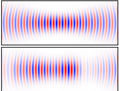
2.6 Electric field distribution around the focus of a Gaussian laser beam. Upper im-age: perfect spatial and time coherence; Lower imim-age: high spatial coherence,
poor time coherence. 9
2.7 Basic set-up of a dual beam partial coherence interferometer. From [15]. 10
2.8 Measurement example. From [22]. 11
2.9 Ultrasound biometry procedure set-up. From [2]. 13
2.10 Scheimpflug principle. From [17]. 14
2.11 Scheimpflug-based imaging. 15
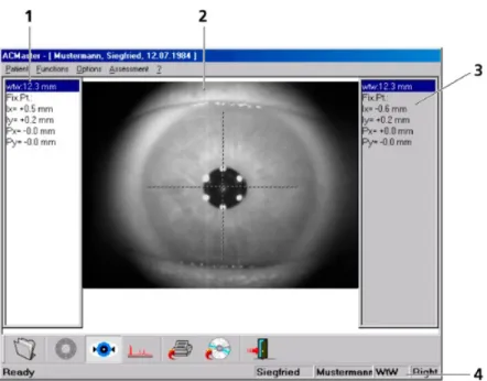
3.1 WtW measurement mode screen: 1 Display field for results of right eye; 2 -Live video image; 3 - Display field for results of left eye; 4 - Status, first name, name, measuring mode and eye (right/left) of live image. From [22]. 19 3.2 WtW alignment: 1 - Image of fixation point; 2 - Image of illumination LED
(reflection point). From [22]. 19
3.3 ACD measurement mode, for Purkinje reflections alignment: 1 - Reflection from anterior corneal surface; 2 Reflection from posterior lens surface; 3 -Reflection from anterior lens surface; 4 - Position of fixation target on internal
LC display. From [22]. 20
3.4 Programmed target shape. 21
3.5 Example of captured image. 22
3.6 Most common artefacts. 24
3.7 Sporadic artefacts. 24
3.8 Artefacts resulting from misalignment. 24
3.9 Misalignment examples. 25
3.10 3P appearing within consecutive frames. 25
3.11 Procedure to make detected third Purkinje reflection (green outline) follow ar-row’s path, so that it overlaps first Purkinje reflection 27 3.12 Dependencies between movements in predicting third Purkinje reflection
move-ment. 28
3.13 Programmed line in Labview to test OLED rotation. 29 3.14 Programmed line’s starting and final positions for OLED rotation calculation. 30 3.15 Test eye and goniometer mounted in the AC Master for eye tilt measurements. 31
3.16 Measuring test eye tilt. 33
3.17 Third Purkinje location changes with fixed target. 34 3.18 Transformingd~pt intod~
Op, andd~Opintod~3P. 37
3.19 d~
pt givesd~3Pthrough rotation byφ and scaling byβ. 37
4.1 Variance filter on original image. 40
4.2 Grayscale values along depicted yellow line, before and after static level
thresh-olding. 40
4.3 Connected components object detection. 41
4.4 Detected objects for inter-frame connectivity. 42
4.5 Original frames example considered for NCC. Grid pattern for NCC also shown. First Purkinje reflection can be seen to move slightly. 43
4.6 Detected third Purkinje reflections. 43
4.7 Eccentricity values to distinguish between first Purkinje reflections. 44
4.8 Detected regions with movement. 45
5.1 Reading image into Matlab. 47
5.2 Coarse first and third Purkinje reflections separation. 48
5.3 Isolating first Purkinje reflection. 48
5.4 Cropping area of interest. 49
5.5 Isolating third Purkinje reflection. 49
5.6 Third Purkinje reflection detection final criteria. 50
5.7 Detection in misalignment. 51
5.8 Other detection problems. 51
5.9 Separation between first and third Purkinje reflections as a resul of test eye tilting. 55
5.10 Distance vs. Absolute angle. 55
5.11 Detected third Purkinje reflection’s location with fixed target. 57 5.12 Calculated vs. Original target locations, detail. 58
2.1 Measurement modes and their symbols. From [22]. 6
4.1 Methods and main results for background/foreground differentiation approach. 42
5.1 Measurements and results for OLED rotation angle calculations. 52 5.2 Measurements and results for angle step calculations. 53 5.3 Linear regression coefficients for horizontal and vertical movements’ plots. 56 5.4 Statistics for third Purkinje location as the eye looks at a fixed target. 57
6.1 Third Purkinje detection and adequate target location calculation efficiency rates. 59
1.1
Project Context
Replacement of the opaque crystalline lens in cataract surgery with an Intra Ocular Lens (IOL) requires intra ocular measurements to calculate the refractive power of the replacement IOL. These measurements include axial eye length, anterior chamber depth along the optical axis as well as measurement of the refractive power of the cornea. Precise interferometry measure-ments of the anterior eye chamber are important for refractive power calculations. Dual beam Low Coherence Interferometry (LCI) is used for these measurements, where alignment of the measurement beam with the eye’s optical axis is of most importance, in order to achieve good measurement sensitivity.
Detection of this axis’ orientation is made with help of Purkinje reflections1. When they overlap, there is alignment of the eye’s optical axis and the illumination beam, and only then can the interferometry measurement beam be used to perform measurements along this same axis with higher sensitivity.
Figure 1.1: Schematic representation of the eye. After [8].
The AC Master from Zeiss Meditec, AG is the instrument used for anterior eye chamber calculations of cataract surgery patients. It incorporates interferometry instrumentation for an-terior eye chamber depth measurements, illumination beam apparatus in order to create Purkinje reflections and a computer connection.
It was used for some time in clinical practice, however there were performance problems concerning alignment between the eye’s optical and visual axes. This alignment is detected when the first and third Purkinje reflections overlap (further explained in next chapter). An 1In this document, to avoid misinterpretations between a digital image and corneal and lens’ reflections, the latter are called Purkinjereflectionsinstead of the most common denomination Purkinjeimages.
operator watches the reflections’ position in the instruments’ external display and makes an interferometry measurement whenever they align. This process has problems in two ways:
• There is a need for a skilled operator (physician).Only an operator who can correctly
identify the different Purkinje reflections and tell them apart from other artefacts in the image can perform this task. This results in high specialization of this work and limits the availability of this procedure, even for cooperative patients.
• Detecting the alignment might not always result in a precise measurement.
Involun-tary eye movements as well as natural lens tilt lead to a great deal of instability on the Purkinje reflections’ location. Therefore, when the operator is making the interferometry measurement, the reflections might have moved again, which leads to axes’ misalignment during measurement and incorrect results.
In conclusion, the process was very unstable resulting in an inability to consistently achieve correct alignment. Therefore, the resulting measurements were unreliable. A new procedure that could more efficiently detect the Purkinje images’ alignment was required.
This project was created in order to research whether such a procedure is possible.
1.2
Document Overview
In order to understand this project’s approach, first a brief introduction to Purkinje reflections will be given in this chapter, along with a short explanation on the necessary measurements, followed by a succinct overview of the AC Master’s components and its performance.
Finally, after having presented this theoretical basis, this project’s approach to the given problem will be laid out.
2.1
Purkinje Images
Purkinje images are formed when light hits the eye’s optical structures. They take their name after Czech anatomist and physiologist Ján Purkynˇe who first described them.
When light hits the eye, the eye’s optical structures reflect the light back. Since there are four optical structures in the eye, which form the cornea and lens, there are also four light reflections, known as Purkinje images number 1, 2, 3 and 4. Figure 2.1(b) shows how they are formed.
• The first two come from the convex surfaces of the anterior and posterior corneal surfaces.
• The third and fourth come from the posterior convex lens’ surface and anterior concave lens’ surface, respectively.
• The first three are erect and virtual images, whereas the fourth image is real and inverted [14].
Looking at an eye in normal day light allows the observer to see the first Purkinje image (coming from the anterior surface of the cornea) on the cornea itself. The other images are normally not visible. To see the other images there mustn’t be much light surrounding the eye, therefore a single illumination beam is the best choice to see the most Purkinje reflections. Fig-ure 2.1(a) shows such an example, a typical Purkinje images image taken with the AC Master.
The first Purkinje image is clearly visible, as well as the third one. The second reflection is overlapping the first one and cannot be distinguished. The fourth reflection is not visible; either it is too dim to be seen or the illumination beam’s angle doesn’t make it possible to be seen. This occurs with most experiments that were performed, therefore the fourth Purkinje reflection will not be discussed in this work. In this work, the first and third Purkinje reflections are the most important.
(a) Purkinje images created with a single illumination beam.
(b) Schematic diagram of the eye. IL - incoming light; A aqueous; C cornea; S sclera; V vitreous; I iris; L lens; CR -center of rotation; EA - eye axis (optical axis). Visual axis not depicted. From [7].
2.2
Eye’s Optical and Visual Axes
An optical axis is defined as the line that connects the centres of reflection and refraction of a centred system. Since the eye is not a centred system, the optical axis is defined as the “best fit” line through the centres of curvature of each reflecting and refracting surface within the eye. For the eye, its optical axis is defined as the line connecting the cornea and lens’s centres of curvature (Figure 2.2). Therefore, the Purkinje reflections’ relative positions are a consequence of the optical axis’ direction relative to the illumination beam [7].
Making the measurement beam go along the same direction as the illumination beam en-sures that when optical axis and illumination beam align, measurement beam and optical axis alignment also occurs. Since the measurement beam is just outside human visible range (850 nm), only the illumination beam is visible to the patient (and only its reflections are seen by the operator).
On the other hand, alignment between the illumination and eye’s optical axes needs to be detected, which is done by an external operator, in order to know when to perform a measure-ment. This alignment setup is achieved by making the patient look at a target. Making the target a single pixel, it also serves the purpose of illumination beam.
The operator can now see the Purkinje reflections, however, only when visual axis and optical axis are close to alignment, meaning that the angle between (known asα - Figure 2.2) them must be very small (results from section 5.2.2 indicate∼1,7◦). In this project, ideally, the patient needs to look in a direction where first and third Purkinje reflections overlapping occurs. This means that the patient’s visual and optical axes are aligned (α is zero).
Figure 2.2: Optical axes of the eye and important angles: [AR] - optical axis; [OF] - visual axis; [OC] - fixation axis; angleα, O ˆNA, between optical and visual axes; angle κ, O ˆPA, between
optical axis and pupillary line [OP]; angle γ, O ˆCA, between optical and fixation axes. From
2.3
The AC Master
2.3.1 Short Instrument Description
The AC Master is a biometry instrument that measures parameters of the anterior segment of the human eye. They include corneal thickness, Anterior Chamber Depth (ACD), lens thickness and eye white width (known as white to white (WtW) measurement). This project concerns the procedure for ACD measurements. The ACD is taken as the distance between posterior corneal surface and anterior lens surface (see Figure 1.1).
These measurements are performed based on optical interference, using a method known as Partial Coherence Interferometry (PCI). It allows detection of interfaces inside the eye, much like an ultrasound A-scan. They are, however, non-contact and much more precise than previous ultrasound methods used for the same purpose[10], [15] (see section 2.4).
In order to perform ACD distance measurements, optical and measurement beam alignment, as well as eye’s optical and visual axes alignment must occur (section 2.2). For the latter, the instrument contains an OLED display which serves for target display, that controls the patient’s fixation direction.
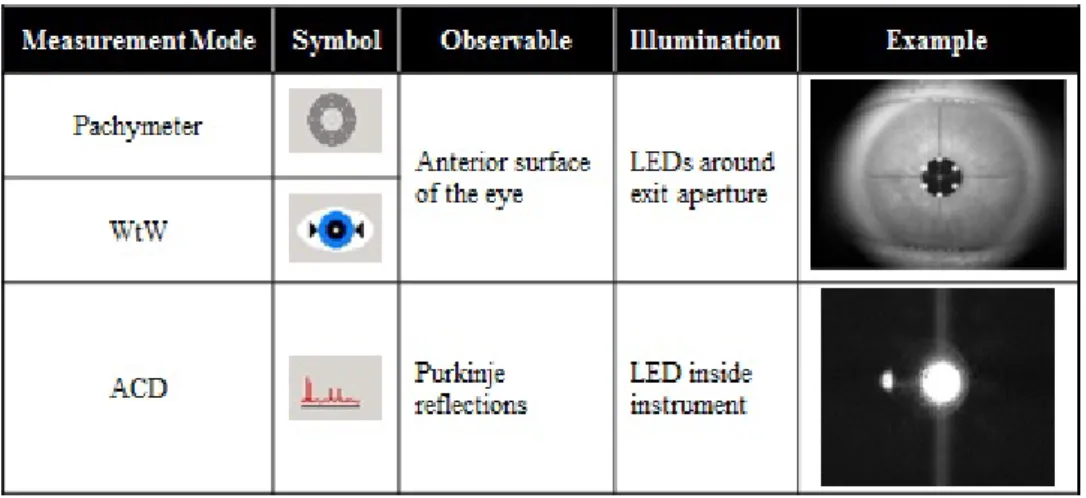
Inside the AC Master there is a CCD camera for observation of the patient’s eye. A backlit external LC display (Figure 2.3, 2) allows observation of the patient’s eye and display of results. There are two possible eye illumination modes, accounting for three measurement modes. Table 2.1 summarizes them.
Table 2.1 Measurement modes and their symbols. From [22].
2.3.2 Basic Operation
The patient rests his head and chin on the instrument’s headrest (Figure 2.5, 4 and 6). The operator uses WtW or pachymeter mode in order to roughly align instrument and eye. More precise alignment of measurement beam and eye’s optical axis is performed in ACD mode, where Purkinje images are observed.
Alignment is initially done with a vertical headrest control (Figure 2.5, 2), in order to very coarsely align the eye with the measurement beam’s exit aperture (Figure 2.5, 7). Afterwards, fine alignment is done through aid of a joystick that moves the instrument in X,Y and Z direc-tions (Figure 2.3, 1).
An external measurement trigger button performs interferometry measurements when pressed (not depicted in Figures 2.3-2.5). Therefore, when the operator decides that adequate alignment is achieved, the button is pressed and a measurement is produced (details on measurements in section 2.4).
Figure 2.3: Operator’s view of the AC Master. From [22].
2.4
Interferometry Measurements
The AC Master performs dual beam interferometry measurements in the eye. This is a type of PCI, using low coherence light from a Super Luminescent Diode (SLD), with 850nm/450µW, to detect interfaces that separate media of different refractive indices within the studied object.
Interferometry is a measurement process that relies on splitting a broadband light source and recombining it again to detect interference patterns after recombination. Spatial and time coherence of the scanning light greatly affect a measurement’s outcome (Figure 2.6). Reducing the light’s time (or spatial) coherence results in higher measurement resolution. Low/Partial Coherence Interferometry (LCI/PCI) is a type of interferometry that relies on this property. However, while temporal coherence affects axial resolution, spatial coherence affects lateral and axial resolution. Early work in LCI showed contrast degradation in result of low spatial coherence [5]. Therefore, low time coherence light is used in PCI.
Figure 2.6: Electric field distribution around the focus of a Gaussian laser beam. Upper image: perfect spatial and time coherence; Lower image: high spatial coherence, poor time coherence.
Axial resolution is defined by the coherence length of a light source. Its lateral resolution depends on the optics used to focus the probe beam onto the sample. A light source’s coherence length,lc, is defined according to the following equation:
lc=
λ02
∆λ (2.1)
Interferometry using coherent light shows interference patterns for distances multiple of co-herence wavelength. Using light with low time domain coco-herence, interference is only detected for waves with path difference smaller than the coherence length of the light, allowing greater measurement resolution and precision[10].
While a conventional Michelson interferometer set-up is sensitive to longitudinal object movements, introducing a second interferometer arm (a so-called dual beam set-up - Figure 2.7) allows total independence from longitudinal movements. A reference structure within the object is used as reference in order to neglect these movements. Therefore, dual-beam interferometry is used in systems that are prone to unavoidable movement and are intrinsically non-static.
Inside the AC Master (Figure 2.7), some parameters of a laser diode are used as light source (LS) in a Michelson interferometer setup [15]. This infra-red beam, with high spatial coherence but very short coherence length, is then split into two components, forming a coaxial dual beam. This dual light beam contains two beam components with a mutual time delay of twice the interferometer arm length difference, 2d, introduced by the interferometer (making this a time domain system). It illuminates the eye, and both components are reflected at several intraocular interfaces.
An interference signal only occurs if the delay of these two light beam components equals an intraocular distance within the coherence length of the light source. This results in measure-ments with very high axial resolution (12µm) and detection precision (.3 to 10µm)[9],[10],[22].
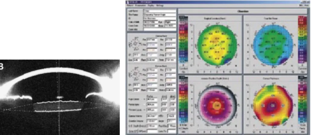
An example of the AC Master’s final measurements are shown in Figure 2.8. A depth scan is performed along the eye’s aligned axes (optical and visual) and interferometry peaks occur whenever the scanning depth matches an interface distance within the eye.
The resulting interference signal in the AC Master is a probing depth vs. relative intensity graphic. Intensity peaks exist whenever an interface is detected along the scanning depth. Lower intensity peaks may also arise from autocorrelation of the strong signal. Figure 2.8 shows such a measurement example. In this graphic, the AC Master automatically indicates the most probable corneal and lens interface peaks:
• ACS - anterior corneal surface;
• PCS - posterior corneal surface;
• ALS - anterior lens surface;
• PLS - posterior lens surface.
Therefore, anterior chamber depth (ACD) is calculated as the xx’ axis value distance be-tween peaks PCS and ALS.
2.5
Project Overview
This project’s main goal is to investigate a novel more user friendly approach to perform accu-rate anterior chamber depth (ACD) interferometry measurements. Perfect alignment between the eye’s optical axis and its visual axis is of greatest practical importance, since precise mea-surements can only be acquired in such conditions. This new approach will rely on having the subject focus on a moving target instead of a fixed one.
Previously, the subject was asked to focus his gaze on a fixed target - a lit pixel on the AC Master’s internal OLED. The light coming from this pixel would reflect on the eye’s optical surfaces and create the desired Purkinje reflections. The technician would then adjust the in-strument’s position (using the joystick) in order to make the Purkinje reflections overlap [22], meaning that the eye’s optical axis is aligned with the measurement beam.
Accommodation of the patient, involuntary eye movements, natural lens tilting and techni-cian’s inexperience would make overlapping the reflections very difficult.
A different method was devised in order to improve measurement conditions. Instead of having the subject focus on a fixed target, the patient is asked to focus on a target as it moves.
A pixel is lit for a fixed time, then another is lit while the previous is turned off. In this way, the subject sees the target moving. Therefore, the eye’s optical axis changes orientation as the target moves, changing the Purkinje reflection’s relative positions. This method would eliminate accommodation difficulties that previously existed from focusing on a fixed target. The pixel illumination sequence is programmed to form a spiral pattern (see section 3.3).
The CCD camera sends live Purkinje reflections video to the computer. The video’s image sequence is then subject to image analysis in order to differentiate the reflections. The main goal would be to detect the third Purkinje reflection in every image, therefore following its movement. Whenever the third reflection is detected overlapping the first one, the OLED’s lit pixel position should be recorded as a good measurement position.
If, however, no overlapping is detected in the considered sequence, this approach is not useful. A new method was devised in order to calculate an adequate measurement position in case overlapping is not detected.
2.6
State of the Art
There are currently three main technologies in ACD measurements: interferometry-based in-struments (which is the AC Master’s category), ultrasound-based measurements and Scheimpflug principle-based imaging. The first two technologies are very closely related, given that both work on the basis of detecting waves that reflect off of boundary surfaces. Ultrasound biometry uses sound waves, whereas interferometry employs infra-red light. The latter relies on an opti-cal imaging planes intersection principle, referred to as the Scheimpflug principle (which will be further explained in the following section).
2.6.1 Wave Interference Technology
Prior to interferometry-based measurements, A-scan ultrasound measurements were routine in biometry measurements for precise IOL refractive power calculations in cataract surgery [10].
In order to perform ultrasound measurements of the sampled object, as in any other ultrasound-based medical examination, there must be direct contact between the transducer and the object. Additionally, a transmitting gel has to be used in order to avoid transmission dampening.
These particular set-up requirements imply some procedural disadvantages [2]: first of all, anaesthesia is required for the procedure to be undertaken (see Figure 2.9); transducer contact pressure on the eye can change eyeball shape consequently affecting measurement outcome; contact with gel may give rise to infections. On the other hand, some advantages of ultrasound measurements bring forth some advantages: patient cooperation is required to a lesser extent; this procedure can be used for mature cataracts (dense media).
Figure 2.9: Ultrasound biometry procedure set-up. From [2].
A comparison regarding resolution and precision between both technologies is also required, as is the effective outcome on IOL power calculations.
At 10MHz, the longitudinal resolution of an ultrasound transducer is approximately 200
µm, whereas the resolution of interferometry is aprroximately 12 µm, with precision less than
10µm [10] (as mentioned previously). Ultrasound biometry errors have been shown to be
Some disadvantages of interferometry procedure include [2]: great extent of patient coop-eration required (patient needs to fixate on a target); cannot be used for mature cataracts; and, of course, procedural difficulties arise because of the need to align the eye’s optical and visual axes (which is the main concern of this project).
2.6.2 Scheimpflug-based Imaging
An alternative to wave interference technology, requiring less patient cooperation, is Scheimpflug-based imaging. The Scheimpflug principle states that when the lens plane (LP) and the image plane (IP) of an optical system are not parallel (there is an inclination between both other than 180º), the plane of focus (PoF) is unique and such that all three planes (LP, IP and PoF) meet alongs a single line, called the Scheimpflug line (see Figure 2.10).
Figure 2.10: Scheimpflug principle. From [17].
A Scheimpflug-based imaging technique uses a tilted camera whose PoF is a plane that crosses the eye at an oblique angle, obtaining images that show cross-sections of all structures of the eye up to posterior lens surface depth [13],[16] (see Figure 2.11(a)). Taking images around the eye allows cross-sectional views of the entire anterior chamber. These images are then analysed for tissue boundaries and finally topography images of the cornea is generated, along with determination of ACD.
(a) Example of a Scheimpflug im-age, showing a cross-section of the eye (from cornea to posterior lens surface). From [3].
(b) Example of Scheimpflug-imaging corneal plots. These plots show corneal density and topography. From [13].
3.1
Introduction
A complete procedure to capture and analyse Purkinje reflections and ultimately estimate each subject’s correct target positioning is explained in this section. The complete procedure should follow the following guidelines:
1. Patient’s eye should be properly aligned with the instrument;
2. Patient will follow a focusing target in the instrument in order to make the Purkinje re-flections move; all the while this movement is being recorded;
3. Recorded images are analysed in search for third Purkinje reflection;
4. Results from image analysis are used to estimate correct target positioning.
The AC Master from Zeiss Meditec, AG was used in these experiments. Labview software is used to model the target’s positioning and movement in the instrument’s internal OLED, as well as retrieving and recording videos and images of the resulting Purkinje reflections.
3.2
Aligning Subject and Instrument for Image Capturing
There are two main steps in properly aligning the subject’s optical axis with the instrument’s beam:
I. Coarse alignment of the eye with the instrument’s beam;
II. Fine alignment, with the help of Purkinje reflections.
The following described procedure will hold valid for any alignment made for a test eye (as in Section 3.5.2).
I. Coarse Eye and Instrument Alignment
The subject’s eye has to be aligned with the Exit Aperture of the Super Luminescent Diode (Figure 2.3).
(I.1) Subject places his chin and rests his forehead on the chin and forehead rests (Figure 2.5). Subject should be comfortably seated, so that his breathing and other body movements won’t make his eye move in the operator’s view.
(I.2) Meanwhile, operator turns equipment on. Creates new patient profile (Name, Date of Birth), or accesses an existing one.
(I.3) Measurement mode is automatically initiated after patient profile step is completed. Operator should choose either White to White (WtW) or Pachymeter measurement mode (Figure 3.1, Table 2.1), where live video is shown. Changing between modes is done pressing Tab on keyboard until desired mode is chosen.
(I.4) Operator adjusts eye height relative to Exit Aperture of SLD through rotation of vertical headrest control (Figure 2.5), in order to fully frame the eye inside the live video image.
(I.5) Patient sees yellow fixation target and is asked to focus on it.
Figure 3.1: WtW measurement mode screen: 1 - Display field for results of right eye; 2 - Live video image; 3 - Display field for results of left eye; 4 - Status, first name, name, measuring mode and eye (right/left) of live image. From [22].
I. Fine alignment Using Purkinje Reflections
The operator should now align the subject’s optical axis with the instrument’s beam.
(I.1) Change to ACD measurement mode. The operator will now observe the first Purk-inje reflection and look for the third one (in case it isn’t immediately visible) by moving the joystick. Doing so, he will also align them as best as possible.
(I.2) There should be no forward/backwards movement of the joystick, which would change the previously obtained focus point.
(I.3) Rotating the joystick over itself will move the third Purkinje image closer/further away from the first Purkinje image.
(I.4) Moving the joystick left/right will move the third Purkinje image horizontally. (I.5) The third Purkinje image should be overlapping the first Purkinje image perfectly.
3.3
Capturing Images for Analysis
After aligning subject and instrument, the subject will follow a fixation target programmed through a Labview interface. This interface also allows simultaneous recording of the resulting Purkinje reflections.
3.3.1 Following the Fixation Target Pattern
The subject must focus on a target that he sees as he looks into the exit aperture. The target is a 3 RGB coloured pixel on the OLED. It changes position according to a previously programmed pattern and the subject should follow it. As the eye moves, so do the Purkinje reflections, eventually overlapping.
The target’s movement pattern and speed is programmed in the Labview interface, in order to meet optimal criteria for each patient. It consists of a series of circular loops, starting from the center and going outwards. The loop’s center is the previously determined alignment spot.
Several parameters are programmable, such as the number of loops and position changing speed (how long the pixel remains lit after changing position), etc.
Some scanned portions of the spiral will yield no third Purkinje reflections for a certain subject, whether others are highly dense with reflections. Therefore, a further useful feature allows cropping the target’s complete circular moving pattern into smaller loop quadrants or sections (Figure 3.4(b)) where there is a higher third Purkinje reflections occurrence.
(a) Full spiral, 4 loops. (b) Spiral section, 10 loops.
3.3.2 Image Capturing
Initially, the CCD camera was accessed for video capturing. It was manually enabled and stopped, before starting target movement and after the target finished its programmed path, respectively. This yielded a video containing the Purkinje reflections’ movement as the target followed its path, but also a set of frames prior and after target movement where no target movement happened.
Capturing video in this way did not allow straightforward time correlation between video and programmed target position, since there was no accurate way of knowing which video frame corresponded to the first target position.
Having a good time correlation between video frame and target position is crucial in order to achieve accurate automatic target positioning extrapolation (section 3.5). Therefore, instead of capturing a whole video during each experience, the computer saves the CCD camera image at each instant of target position change.
Additionally, a string array stamp was added to the image, saving the image under that same name. The string contains a time stamp and the target’s X and Y position at that instant. This way, when accessing an image for image analysis, the target’s position at that instant is also known.
3.4
Image Analysis
3.4.1 Image Features
In order to detect the third Purkinje reflection on the recorded images, a series of image features need to be ignored. To understand the chosen method, an introduction of what can be seen in every image and also how it changes from image to image is given.
3.4.1.1 Static
Every captured image is of type double and 480 x 640 pixels, with pixel intensity range [0-255]. The third Purkinje reflection is not present in all images. Some features that appear in every image and must be taken into account while performing image analysis are (Figure 3.6):
• The first Purkinje reflection (1P);
• a white column directly in the middle of the image, resulting from sensor saturation of the CCD camera (C).
There are also artefacts that appear and clearly are not third Purkinje reflections (Figure 3.8). They include:
• A matrix-shaped set of white spots (MS), which are the images of LED’s array in the OLED;
• a halo (H) surrounding the first Purkinje reflection;
• an elongated elliptical shape (ES);
(a) Original image. (b) Artefacts highlighted: 1P - first Purkinje reflec-tion; 3P - third Purkinje reflecreflec-tion; MS - matrix-shaped set of spots; H - halo; C - white column.
Figure 3.6: Most common artefacts.
Figure 3.7: Sporadic artefacts.
(a) Trail of light (TL) can be seen. Elongated elliptical shape (ES) also present.
(b) TL present. Third Purkinje (3P) also present.
(a) An example of misalignment. 1P is very distorted.
(b) An example of misalign-ment. 1P is very distorted. 3P is also visible.
(c) An example of misalignment. 1P is very distorted.
Figure 3.9: Misalignment examples.
3.4.1.2 Motion-related Features
The third Purkinje reflection can be seen changing position along a set of images. It can be absent on an image and appear on the next one (Figure 3.10).
Although it follows a somewhat circular movement pattern in agreement with the moving target, its speed is not constant and can often disappear due to extreme tilting of the eye. Its shape and size often change, overlapping with the white vertical column and other artefacts is common, giving rise to many movement inconsistencies.
Other artefacts also move and change shape, its position change being sometimes more noticeable than the third Purkinje reflection’s. The elongated shape (Figure 3.7) changes shape dramatically very randomly, and the white vertical column can be seen moving from side to side.
In conclusion, there are many objects within the images whose shape, size and position change just as often as the third Purkinje reflection’s. Furthermore, the rate at which these changes occur is not constant. The result is that relying on its movement to detect the third Purkinje reflection will turn out to be very difficult (4.1.2).
(a) Frame # 30. No 3P is visible. (b) Frame # 31. 3P visible.
3.4.2 Final Procedure
An algorithm based on pixel intensity differentiation, connected components size and relative location was ultimately used. This section describes it in more detail.
I. Stored image is read.
At the same time its top is cut off, so that the time and target position stamp is removed, so as to not interfere in pixel intensity differentiation.
II. Coarse pixel differentiation - separating first and third Purkinje reflections.
The first Purkinje reflection can be easily separated by keeping only the highest intensity pixels. This image will be calledfirst Purkinje image.
Performing dynamic thresholding on remaining pixels allows better differentiation of lower intensity pixels. This image will be referred to asthird Purkinje image.
III. Isolate first Purkinje reflection.
Since later on we need to detect the location of both first and third Purkinje reflections, we must make sure that there is only one connected object in previously createdfirst Purkinje image. Therefore, only the largest connected component is kept.
IV. Cropping within area of interest.
One step that can be taken in order to reduce incorrect detection of third Purkinje reflec-tions is to narrow down the search area.
Takingfirst Purkinje image(currently only showing the first Purkinje reflection), create a cropping window centred in first Purkinje reflection, with 280 pixel x 280 pixel size. Cropthird Purkinje imageaccording to this cropping window. This reduces detection of non-third Purkinje reflection pixels that appear farther away from where the third reflec-tion could ever be seen.
V. Detecting third Purkinje reflection.
Taking the now croppedthird Purkinje image, make sure only one connected component is detected.
Every connected object with size larger than a normal first Purkinje reflection is removed. Erosion and dilation is performed to gradually remove small objects. If there are still more than one object detected, remove objects formed by less than 120 pixels.
VI. Final third Purkinje detection criteria.
If the detected third Purkinje object’s is horizontally too close to the first Purkinje object, don’t use it.
3.5
Automatic Target Positioning
An ultimate goal of this project is to calculate where the target should be positioned in order to achieve perfect overlapping of the first and third Purkinje reflections. When no overlapping is detected through image analysis, the relationship between third Purkinje reflection movement as the eye rotates while following the target must be known.
Figure 3.11: Procedure to make detected third Purkinje reflection (green outline) follow arrow’s path, so that it overlaps first Purkinje reflection
The subject focuses his eye on a target which is a light spot in the OLED inside the AC Master. As the spot moves, the eye follows it and there’s a corresponding movement of the Purkinje reflections.
A known feature of the OLED inside the AC Master is that it is not fitted perfectly straight. The display is rotated, resulting in a rotation of the target’s movement from the originally pro-grammed. Furthermore, one must know how the third Purkinje reflection moves as the eye moves. Therefore, there are at least two variables one must take into account when calculat-ing where to place the target in order to make the third Purkinje reflection overlap the first one (Figure 3.11). These relationships have to be determined in order to know how the Purkinje reflections relate to the target’s movement (Figure 3.12).
Two experiments were set up in order to calculate the OLED’s rotation inside the AC Master and how the third Purkinje reflection moves as the eye moves.
A third experiment was also performed, in order to determine the error associated with the third Purkinje reflection’s location.
3.5.1 OLED Rotation
3.5.1.1 Measurements
Instead of programming a single spot in the OLED, a line segment was programed in Labview to appear in the OLED (Figure 3.13). Two points are programmed as endpoints of that line segment (X1, Y1 - left; X2, Y2 - right). The right endpoint is fixed, the left one moves with arrow keys keystrokes on the AC Master keyboard.
1. With the AC Master already turned on and communicating with the computer, run pro-gram on Labview that makes a line segment appear in the OLED (Figure 3.13).
2. Subject should place his head and chin comfortably on chin and headrests of the AC Master (Figure 2.5).
3. Subject should adjust eye height with vertical head rest control (Figure 2.5) in order to perfectly see line segment inside the AC Master.
4. Subject should use arrow keys on AC Master’s keyboard to move left extremity and make line segment as horizontal as possible.
5. Record coordinates of X1, Y1 point.
6. Repeat for several subjects.
3.5.1.2 Data Analysis
Figure 3.14 depicts the scheme to calculate the OLED rotation inside the AC Master. When the line is in the final position, the subject sees a horizontal line in the AC Master’s OLED. Results and final calculations in section 5.2.1.
cosφ = |FinalPosition| |StartingPosition|
=
p
(X1,last−X2,f irst)2+ (Y1,last−Y2,f irst)2
p
(X1,f irst−X2,f irst)2+ (Y1,f irst−Y2,f irst)2
(3.1)
3.5.2 Purkinje Reflections Separation vs. Eye Tilt
A test eye1attached to a goniometer (Figure 3.15) was mounted on its corresponding mounting
spots in the AC Master’s headrest (Figure 2.5,5), to study the third Purkinje reflection’s as the eye tilts.
Figure 3.15: Test eye and goniometer mounted in the AC Master for eye tilt measurements.
3.5.2.1 Measurements
I. Setting Up the System
(I.1) With the AC Master already turned on and communicating with the computer, run video capturing program that will show CCD camera live video (the same that is seen in the AC Master’s external OLED, Figure 2.3,2).
(I.2) Mount test eye in the AC Master (Figure 2.5,5). Be sure that eye side is as parallel to mounting beam as possible, which will help with initial test eye alignment. Also make sure that the goniometer reads 0°.
(I.3) Adjust vertical head rest control (Figure 2.5), placing test eye as close to Exit Aper-ture of SLD (Figure 2.5) as possible.
(I.4) Now the test eye should be aligned with the measurement beam, in the same way done in section 3.2.
(I.5) Once it is correctly aligned, this alignment can be checked. Still in ACD ment mode, use the interferometry measurement button to check if a good measure-ment is done. This ensures that there is an adequate alignmeasure-ment between the test eye’s optical axis and the measurement beam.
II. Tilting and Recording Measurements
(II.1) Using the goniometer handle, tilt the eye in small steps. Take a snapshot of the cap-tured video (Figure 3.16(a)), for further image analysis to calculate distance between first and third Purkinje reflections.
(II.2) Repeat tilting and taking snapshots, until reaching tilt where third Purkinje reflection is no longer visible.
(II.3) Once the reflection has disappeared, continue tilting the eye in the opposite direction and taking snapshots at each tilt.
3.5.2.2 Data Analysis
Since the measurable angle range was very small and the goniometer scale too large for the performed tilts, it was not possible to record the angle where each snapshot was taken. Instead, recording maximum and minimum angles was the devised method. This way, taking the number of snapshots between these extremities, a rough angle step estimation can be calculated.
Therefore, letθ1andθ2be extremities angles,s1ands2be first and last snapshot. The angle
step,θstep, is thus
θstep = ∆
θ
∆s = θ2−θ1
s2−s1 (3.2)
Image analysis on these images was performed simply by detecting highest intensity pix-els, after performing Otsu’s threshold. Since the test eye is made with glass lenses, there are less artefacts present than in a normal human eye would be. Both the first and third Purkinje reflections were regions of very high intensity pixels, enabling a very straightforward detection procedure.
(a) Example of a snapshot. (b) Resulting horizontal move-ment.
Figure 3.16: Measuring test eye tilt.
3.5.3 Eye Fixation Deviation
A subject stared at a fixed target in the AC Master’s OLED for some time, and a video was recorded. This video was then subject to image analysis to detect the third Purkinje reflection. In this way, we can see how precise is the location of the third Purkinje reflection when looking at a target. Figure 5.2.3 shows how the third Purkinje reflection moves even when the eye is fixating a target.
(a) Detected third Purkinje far-ther away from first Purkinje.
(b) Detected third Purkinje closer from first Purkinje.
Figure 3.17: Third Purkinje location changes with fixed target.
3.5.4 Final Calculations
For each pair of detected third Purkinje reflections and corresponding detected first Purkinje reflections, their
Therefore, given two images,k1andk2, where third Purkinje reflections were detected, let:
• ~d
jbe the displacement vector of either programmed target (pt), OLED pixel (Op), first or
third Purkinje reflection (1P, 3P) (j={pt;Op; 1P; 3P});
• xj,kandyj,k be j’s x and y coordinates on imagei(k={k1;k2});
• φ be the calculated OLED rotation (from section 3.5.1);
The goal of the following equations is to find the relation between the tilt of the eye (which is to say, its visual and optical axis) and the corresponding displacement of the fixation target in the OLED.
Vectord~
Op is a rotation of vector d~pt, given that the OLED is rotated φ degrees inside the
AC Master. It is assumed that no shrinkage or expansion occurs. Therefore, in complex space, we have,
~
dOp=d~pt·exp(φi) (3.3)
as seen in Figure 3.18(a).
On the other hand, having studied third Purkinje reflection’s movements as the eye rotates, we know that its displacement vector must be a function of the OLED pixel’s displacement. It was shown that this is a linear relation (section Results and Discussion). Therefore,
~
d3P=β·d~Op (3.4)
as seen in Figure 3.18(b).
Combining both equations (3.3 and 3.4), we have the relationship between third Purkinje reflection and programmed target to be,
~
d3P=β·d~pt·exp(φi) (3.5)
as seen in Figure 3.19.
Given that the angle change occurs due to Labview-OLED transformation, we take thatβ
can be calculated as follows,
Therefore, knowing the programmed target’s and third Purkinje reflection’s coordinates on both images, we have,
|d~3P|=
p
(x3P,k2−x3P,k1)2+ (y3P,k2−y3P,k1)2
|d~pt|=
q
(xpt,k2−xpt,k1)2+ (ypt,k2−ypt,k1)2
β = |d~3P| |d~pt|
(3.7)
On the other hand, in cartesian space, the third Purkinje reflection’s and target movement’s equations are as follows,
x3P,k2=x3P,k1+∆x3P
y3P,k2=y3P,k1+∆y3P
Xpt,k2=Xpt,k1+∆Xpt
Ypt,k2=Ypt,k1+∆Ypt
(3.8)
Accordingly, in cartesian space, equations 3.3 and 3.4 can be written as,
(
∆xpt =∆xOp·cosφ
∆ypt =∆yOp·sinφ
(3.9)
and,
(
∆x3P=∆xOp·β
∆y3P=∆yOp·β
(3.10)
again, assuming a linear relation between OLED pixel’s movement and third Purkinje re-flection’s movement (no rotation).
Taking equations 3.9 and 3.10, and solving it for∆xpt and∆ypt, we have,
(
∆xpt=∆x3P·cosβφ
∆ypt=∆y3P·sinβφ
(3.11)
∆x3P=x3P,k1−x1P
∆y3P=y3P,k1−y1P
xpt,new=xpt,k1+∆x3P·cosβφ
ypt,new=ypt,k1+∆y3P·sinβφ
(3.12)
In conclusion, in order to estimate new target coordinates (xpt,new,ypt,new) for better
align-ment, we have,
(
xpt,new=xpt,k1−(x1P−x3P,k1)·cosβφ
ypt,new=ypt,k1−(y1P−y3P,k1)·sinβφ
(3.13)
whereβ is given by equation 3.7.
(a) Rotatingd~ptbyφgivesd~Op. (b) Scalingd~Opbyβgivesd~3P.
Figure 3.18: Transformingd~pt intod~
Op, andd~Op intod~3P.
Figure 3.19: d~pt givesd~3
Working on how to detect the third Purkinje reflection was the most time consuming step of the project. The results of this research ultimately changed this project’s approach to achieve optical axis and measurement beam alignment. Chapter 3 already presented the final chosen approach, therefore this chapter will comprise a summary of tested image analysis approaches that proved ineffective.
Since these approaches were not ultimately used, a short discussion on their results and effectiveness within this project’s framework is also presented in this chapter, rather than being dispersed in chapters 5 and 6, which are dedicated only to actually used approaches.
4.1
Searching for an Optimal Image Analysis Procedure
The first step every image analysis algorithm should undergo is applying adequate image thresh-old. Reducing image noise level improves the chances to detect meaningful regions within the image.
Differentiation of regions within the image, however, can be achieved through a multitude of methods. In this project, the main tested approaches dealt with frame differentiation and shape differentiation.
4.1.1 Pre-Analysis
Thresholding the recorded images is the first step to be taken.
Every picture had a slightly different gray value histogram profile, therefore a single thresh-old level (static level threshthresh-olding) for every image from every experience would not yield a good noise reduction performance.
Matlab’s Otsu dynamic threshold proved simple and effective in reducing noise level ac-cording to each image’s distinct gray level histogram, and it was ultimately used.
Variance filter was also tested in a pre-analysis context (Figure 4.1). This is a filter that allows regions border’s detection. However, border detection at this analysis level was not the most helpful method, given that border definition was very fuzzy and didn’t allow clear region distinction - it proved more helpful for shape refinement at a higher image analysis level.
Figure 4.2 shows an example of how static level thresholding reduces image noise level. Along the yellow line (going through the third Purkinje reflection), there is significant gray value reduction after threshold. This results, however, were not consistent for every image, many times eliminating third Purkinje reflections when they were fainter.
Figure 4.1: Variance filter on original image.
(a) Original image. (b) After threshold.
(c) Gray value before threshold. (d) Gray value after threshold.
4.1.2 Detecting the Third Purkinje Reflection
4.1.2.1 Object Detection in Matlab
After thresholding, there is a sharper distinction of meaningful objects.
Matlab provides a pixel aggregation method that groups pixels together based on their close-ness. In this way, adjacent non-zero pixels form an object (Figure 4.3). Therefore, an object is a region within an image where all pixels have pixel intensity different than zero. However, inside a given area there can be many different pixel intensity regions.
(a) 2 objects detected. (b) 1 object detected.
Figure 4.3: Connected components object detection.
These areas are called connected components objects. They can now be differentiated from one another within a single image (Shape Differentiation approach) or along a series of images (Foreground/Background Differentiation approach). The first approach relies on shape, size or pixel intensity differences of all the different objects in one image, the latter aims at spotting moving objects within a set of images.
Both approaches have been extensively researched in the field of image analysis. The fol-lowing sections list the ones that were tested for this project’s purpose.
4.1.2.2 Foreground/Background Differentiation
Foreground/background differentiation methods are very popular in order to detect moving ob-jects within a set of images [4],[?],[6],[19],[20]. Some researched methods were:
• Frame difference [21];
• frame averaging;
• inter-frame connectivity;
• using Normalized Cross-Correlation (NCC) to detect regions with most movement [11],[18].
Other tested methods were Gaussian Mixture Model based tracking [12] and variance filter along a number of images. These approaches, however, took too much computing time and no results were actually achieved.
Table 4.1 Methods and main results for background/foreground differentiation approach.
(a) Previous frame. (b) Current frame.
(a) Previous frame. (b) Current frame.
Figure 4.5: Original frames example considered for NCC. Grid pattern for NCC also shown. First Purkinje reflection can be seen to move slightly.
4.1.2.3 Shape Differentiation
Another possibility to differentiate the third Purkinje reflection from other detected objects within an image would be its size, shape or pixel intensity profile.
The third Purkinje reflection pixel intensity profile changes dramatically within a set of images, sometimes being very faint and barely distinguishable from the background, other times having a rather self-differentiating pixel intensity. Whereas the first Purkinje reflection always has the same high intensity pixel value, this feature could not adequately differentiate third Purkinje reflections.
The third Purkinje reflection’s size also proved to be an inadequate differentiating feature. This is also a consequence of its changing pixel intensity profile - a smaller third Purkinje reflection usually derives from lower pixel intensities.
Matlab provides an Eccentricity measurement for connected components within an image. It measures whether an object is more closely shaped to a line segment (Eccentricity=1) or a circle (Eccentricity=0). However, as shown on Figure 4.6, third Purkinje reflection’s shape changes considerably, therefore not allowing to be detected in this way.
(a) Larger and elliptical-shaped. (b) Smaller and round-shaped.
Shape differentiation through Eccentricity measurements was also tested for good first Purk-inje reflections detection, i.e., to discard images where the first PurkPurk-inje reflection was distorted due to misalignment.
Figure 4.7 shows two distinct first Purkinje reflections. On Figure 4.7(a), we see a reflection created due to poor misalignment, on Figure 4.7(b) there is an acceptable reflection. Eccentricity measurements for both these situations are however very similar; there isn’t enough difference to use this feature as a differentiating tool. Similar results happened for third Purkinje reflections differentiation.
(a) Eccentricity=0,4927 (b) Eccentricity=0,4114
4.2
Results and Discussion
Figure 4.8 shows an example of detected objects/areas by these methods. The pink areas are detected regions throughout a whole set of images. The white area is the current frame after thresholding.
Analysing this image, it is clear that most of detected areas are where artefacts occur. Most importantly, the white vertical column is the most commonly detected region. There is not a sufficiently high third Purkinje reflection detection rate.
Figure 4.8: Detected regions with movement.
Foreground/background differentiation methods detected fast moving objects within a set of images. Whether with frame averaging, NCC or frame difference, artefacts were the fastest moving objects in an image set. This happened because their borders were constantly changing, at a much higher rate than the third Purkinje reflection.
This meant that artefacts had a high detection rate, whereas the third Purkinje reflection, while detectable, wasn’t differentiated at a high enough rate to deem these methods effective. To overcome this problem, a movement speed threshold could be implemented. However, the third Purkinje reflection’s movement is very erratic and random, meaning that such a method would most probably be ineffective.
Differentiating third Purkinje reflections based on their pixel intensity profile, size or shape was clearly ineffective, given that none of these features are constant for a third Purkinje reflec-tion (although they are for the first Purkinje reflecreflec-tion).
5.1
Image Analysis
5.1.1 Final Procedure I. Stored image is read.
Taking the original stored image, reading it into Matlab and cutting time and target position stamp rectangle from the top, so as to not interfere in image analysis.
Figure 5.1 is an example of this procedure: on the right is the original image with time and target position stamp; on the left, the image (referred to asimage)that is going to be analysed on Matlab.
(a) Original image. (b) image.
Figure 5.1: Reading image into Matlab.
II. Coarse pixel differentiation - separating first and third Purkinje reflections.
Since the first Purkinje reflection saturates the CCD camera, it can be easily removed in order to increase the contrast of the rest of the image.
Isolating the first Purkinje reflection image indeed proved to be very efficient: simply taking the highest intensity pixels (gray scale value=1, seen in Figure 5.2(a)) onimageand storing it in an image calledfirst_purkinje. This image can, however, still have some random small regions that are also of high intensity. They will be easily removed later, on stepIII.
Detection of third Purkinje reflection will now be done on an image that results from sub-tracting first_Purkinje on image. Dynamic thresholding is performed on this difference im-age, for better differentiation of different pixel intensity regions. The resulting image is called third_Purkinje(Figure 5.2(c)).
Figure 5.2 shows normal results for this step.
(a)first_purkinje (b) first_purkinjeandimage difference
(c)third_purkinje
Figure 5.2: Coarse first and third Purkinje reflections separation.
III. Detecting first Purkinje reflection.
As previously mentioned, first_Purkinje may in some cases still have more than one con-nected component object (which is not the case for this example, Figure 5.3(a), where only one object existed from the beginning). Only the largest object is kept, successfully detecting the first Purkinje reflection.
(a) first_purkinje.
IV. Cropping within area of interest.
Cropping first_Purkinje within an area of size 280 x 280 pixel centred on the detect first Purkinje reflection’s centroid (Figure 5.3(a)). third_Purkinje(Figure 5.4(b)) is cropped around the same area.
This prevents detection of regions that could be mistaken by the algorithm as third Purk-inje reflections, but appear much farther away from the first PurkPurk-inje reflection than the third Purkinje reflection could.
(a) first_purkinje (b) third_purkinje
Figure 5.4: Cropping area of interest.
V. Third Purkinje reflection detection.
third_Purkinjestill has many connected components that need to be discarded.
No shape, size or pixel intensity criteria can be used (as previously discussed in section 4.1.2.3), therefore only objects that are too big to be a third Purkinje reflection are removed. In this way, objects bigger than a normal first Purkinje reflection are ignored.
Through a few steps of image erosion and dilation, objects boundaries are more defined and smaller objects are gradually removed. Objects that are still too small (formed by less than 120 pixel), are now removed, much like when detecting only one first Purkinje reflection.
Figure 5.5(a) is an example where, after removing objects too big and smaller objects, only one object remained.
(a)third_purkinje
VI. Final third Purkinje reflection detection criteria.
Most of the times, third_Purkinje still has more than one object after the previous step. Studying these images, most of the non-third Purkinje objects detected were segments of the vertical white column artefact (Figure 5.6(a)). Therefore, an implemented final criteria for better third Purkinje reflection detection was to remove all objects whose centroid was horizontaly too close to the detected first Purkinje reflection’s centroid.
Figure 5.6(a) is an example of a detected object that clearly is not a third Purkinje reflection. In this case, no reflection is detected, even though one is clearly seen below the first Purkinje reflection but hovering over the white vertical column. Since it was not differentiated from the vertical white column in previous steps, it will not be detected.
Figure 5.6(b) is an example of an object that can be kept, because its centroid was not too close to the first Purkinje reflection’s centroid.
(a) Reject. (b) Accept.
5.1.2 Detection Problems
One problem that still occurs is some third Purkinje reflections are detected when there is mis-alignment of illumination beam and eye’s optical axis.
As previously discussed, attempts at discarding situations where misalignment occurs were not possible (section 4.1.2.3), with shape differentiation. No other method proved to be efficient. Therefore, there are still situations where detection can occur in misalignment, as seen in Figure 5.7.
(a) (b)
Figure 5.7: Detection in misalignment.
Finally, other occasional detection problems occur that are not so easily avoidable. An example of this is Figure 5.8. In this case, an object smaller than a first Purkinje reflection whose centroid was not horizontally close to the first Purkinje reflection was detected. However, it was clearly not a third Purkinje reflection.
(a) Incorrectly detected third Purkinje.
(b) Detail, after subtrac-tion of first Purkinje.
5.2
Automatic Target Positioning
5.2.1 OLED Rotation
Three subjects were used for calculation of OLED rotation inside the AC Master. The results are in Table 5.1.
Accordingly,φ = 16,7◦was used for calculations that called for this angle.
5.2.2 Purkinje Reflections Separation vs. Eye Tilt
5.2.2.1 Angle Step Calculation
A third Purkinje reflection from the test eye can be seen whenθ ∈[-1,7; 1,7]◦. This is a very
small range, and the goniometer’s scale did not allow registering every angle’s position for each step.
Using Equation 3.2, every angle θ step could be calculated in order to derive a better eye
tilt vs. third Purkinje reflection location relationship. Table 5.2 shows these results for both horizontal and vertical tilting.

![Figure 2.2: Optical axes of the eye and important angles: [AR] - optical axis; [OF] - visual axis;](https://thumb-eu.123doks.com/thumbv2/123dok_br/16548155.737034/21.892.244.650.714.890/figure-optical-axes-important-angles-optical-axis-visual.webp)
![Figure 2.3: Operator’s view of the AC Master. From [22].](https://thumb-eu.123doks.com/thumbv2/123dok_br/16548155.737034/23.892.214.676.533.812/figure-operator-s-view-ac-master.webp)
![Figure 2.5: Patient’s view of the AC Master. From [22].](https://thumb-eu.123doks.com/thumbv2/123dok_br/16548155.737034/24.892.212.674.528.751/figure-patient-s-view-ac-master.webp)
![Figure 2.7: Basic set-up of a dual beam partial coherence interferometer. From [15].](https://thumb-eu.123doks.com/thumbv2/123dok_br/16548155.737034/26.892.231.658.649.942/figure-basic-set-dual-beam-partial-coherence-interferometer.webp)