MASS CONSERVATION ENHANCEMENT OF FREE BOUNDARY FLOWS IN COMPOSITES MANUFACTURING
Zuzana Dimitrovová
zdimitro@dem.ist.utl.pt
IDMEC/IST and DEM/ISEL
Av. Rovisco Pais, nº 1, 1049-001 Lisbon, Portugal
Suresh G. Advani
advani@udel.edu
Department of Mechanical Engineering, University of Delaware 126 Spencer Lab, Newark, DE 19716, USA
Abstract. Undesirable void formation during the injection phase of the liquid composite molding process can be understood as a consequence of the non-uniformity of the flow front progression, caused by the dual porosity of the fiber perform. Therefore the best examination of the void formation physics can be provided by a mesolevel analysis, where the characteristic dimension is given by the fiber tow diameter. In mesolevel analysis, liquid impregnation along two different scales; inside fiber tows and within the spaces between them; must be considered and the coupling between these flow regimes must be addressed. In such case, it is extremely important to account correctly for the surface tension effects, which can be modeled as capillary pressure applied at the flow front. When continues Galerkin method is used, exploiting elements with velocity components and pressure as nodal variables, strong numerical implementation of such boundary conditions leads to ill-posing of the problem, in terms of the weak classical as well as stabilized formulation. As a consequence, there is an error in mass conservation accumulated especially along the free flow front. This article presents a numerical procedure, which was formulated and implemented in the existing Free Boundary Program in order to significantly reduce this error.
1. INTRODUCTION
Liquid Composite Molding (LCM) processes such as Resin Transfer Molding (RTM), Vacuum Assisted Resin Transfer Molding (VARTM) and Vacuum Assisted Resin Infusion (VARI) are widely used to manufacture advanced composites with continuous fiber reinforcements (Advani et al, 1994). They belong to a class of low injection pressure processes in which a pre-placed dry fiber preform is held stationary in the mold (the mold can have two rigid faces or one rigid and one flexible face) and a thermoset resin is injected into it to cover the empty spaces between the fibers. Resin infiltration into the fiber preform must be carefully controlled in order to avoid poor wetting and to minimize residual voids content, which can be detrimental to the performance of the fabricated parts. Resin can be allowed to cure only after the injection is complete. Therefore one of the main objectives of the related fluid flow analysis is the determination of the free boundary advance pattern, together with the identification of regions of probable voids or dry spots occurrence.
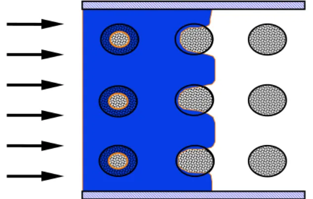
The continuous fiber reinforcements, called fiber preforms, consist of bundles of 2000 to 5000 fiber filaments, commonly known as fiber tows. The fiber tow is usually millimeters in diameter and consists of filaments of about 7 to 20 micrometers in diameter. Fiber tows are usually knitted, woven or stitched together, forming in this way dual porosity medium (Fig. 1). Due to this dual porosity, resin progression is not uniform, and a transition region where the flow is not yet stabilized and which is very sensitive to voids formation, is formed along the macroscopic flow front. The best way to analyze this region is by the mesolevel analysis, i.e. at the scale of the fiber tows (Advani and Dimitrovová, 2004), (Dimitrovová and Advani, 2004b).
Figure 1 – Top view of fiber preform consisting of woven fiber tows (each fiber tow contains 3000 individual fiber filaments). Photograph on the left and a schematic on the right.
At the mesolevel two different flow regimes, corresponding two different scales: Stoke’s flow in the inter-tow spaces and Brinkman’s flow within the fiber tows must be linked together. Fiber tows can be replaced in such analysis by single porous media with uniformly spaced pores and Brinkman’s regime will reduce to Darcy’s law in certain small distance from the tow surface. Capillary pressure correct implementation in mesolevel simulations is extremely important and in the inter-tow spaces must correspond to the actual curvature of the flow front, while homogenized value should be used within the fiber tows. When continues Galerkin method is used, exploiting elements with velocity components and pressure as nodal variables, strong numerical implementation of such boundary conditions leads to ill-posing of the problem, in terms of the weak classical as well as stabilized formulation. As a consequence, there is an error in mass conservation accumulated especially along the free flow front. This error can affect significantly not only the global mass conservation, but also the normal velocities at the free front and consequently distort the next front shape. If the
explicit integration along the time scale is implemented, such errors are irreversible. Techniques of reducing this error significantly will be shown in this article; their implementation in the already existing Free Boundary Program (FBP) enhance this software in a way that it is capable of reproducing the necessary resin flow dynamics in LCM filling simulations at the mesolevel.
2. MESOLEVEL ANALYSIS
2.1 Basic flow situations
The understanding of the flow physics in mesolevel simulations can be separated into two basic flow situations: flow across and along fiber tows. In the case of flow across the fiber tows, experimental evidence shown in (Parnas and Phelan, 1991), (Parnas et al, 1994) and (Sadiq et al, 1995) and numerical results presented in (Spaid and Phelan, 1998), (Dimitrovová and Advani, 2003, 2004a) clearly demonstrate that filling of the fiber tows is delayed. Resin advance, although helped by strong intra-tow capillary pressure, must overcome a fiber arrangement with very low intra-tow permeability; thus there could hardly exist some scenario, which would move the front more or less uniformly (Fig. 2). It is also known (Potter, 1997) that very high surrounding pressure acting on the tows can significantly change the single fibres positions and actually close some spaces between them. Usually only a thin strip along the fibre tow circumference is filled when the primary resin front envelopes it, then the air is compressed inside the tow until it is balanced with the surrounding resin pressure. Hence the capillary action becomes the only factor that can drive the resin inside the tow. When the air pressure becomes higher than the surrounding pressure, the air can escape from the tow in the form of microvoids.
Figure 2 – Schematic of flow across fiber tows.
In flow along fiber tows, permeability is much higher (four to ninety times) and capillary action is generally twice as strong as in flow across the tows. Therefore two situations can be found in flow along fiber tows (Patel and Lee, 1995), (Patel et al, 1995) and (Binetruy, 2000). Wicking flow front inside the fiber tow can be either advanced or delayed with respect to the primary front in the inter-tow spaces, which also pre-determinates the location and shape of the emerging voids (Fig. 3).
to the hydrodynamic pressure gradient and therefore inter-tow spaces (the higher permeability regions) are filled first. On the other hand, under lower externally applied action, wicking flow can become dominant and resin advances more rapidly inside the tows. There must naturally exist a situation, when these actions are “equilibrated” and resin progresses more or less uniformly. It should be remarked in this context, that higher external conditions are used with the objective to reduce the filling time, as a main cost factor. On the other hand it is well known that lower external conditions are favorable for better accomplishment of the infiltration phase and quality of the part, because sufficient time must be given to the resin-fiber interaction to form an interface increasing the adhesion between the two phases. However, in very slow filling it is conceivable that the resin will cure and solidify before all the empty pores are filled.
Figure 3 - Inter-tow (a) and intra-tow (b) void formation.
More about role of capillary driven flow in composites manufacturing can be found in (Advani and Dimitrovová, 2004). In summary, it is obvious that in modeling of physics of the voids formation it is extremely important to account correctly for the capillary pressure influence.
2.2 Flow domain and governing equations
In the mesolevel analysis single scale porous media (fiber tows, represented in Fig. 4 by grey half-circles) and open spaces (white spaces), are presented together in the flow domain. Fiber tows have uniformly distributed pores, therefore the sharp flow front can be assumed while the resin impregnates. As the flow is slow, inertia terms can be neglected, implying that one can assume Stoke’s flow in the currently filled inter-tow spaces St
k
Ω (white space between Γin and tS
k
Γ ) and Darcy’s flow in the saturated intra-tow region Bt
k
Ω , which need to be coupled and solved at each discretized time tk (Fig. 4). In fact, Darcy’s law must be
modified to Brinkman’s equations, in order to account for the viscous stress at the interface
Flow direction
Flow direction
a)
between these two regions ( S B tk
−
Γ ). Viscous stress rapidly decreases with the distance from
B S tk
−
Γ , i.e. the domain, where the Brinkman’s term is important, forms only a thin strip around the fiber tow surface. In summary, the following equations must be fulfilled at each time step, tk:
Stoke’s equations in the inter-tow spaces:
0
= ⋅
∇ v and ∇p=μΔv in St
k
Ω , (1)
Brinkman’s equations in the intra-tow spaces: 0
D =
⋅
∇ v and ∇pf =μΔvD−μK−1⋅vD in Bt
k
Ω , (2)
where v is the local velocity vector, p is the local pressure, μ is the resin viscosity and ∇ stands for the spatial gradient, Δ=∇⋅∇. vD is the Darcy’s velocity vector, i.e. the phase averaged velocity related to the intrinsic phase average vf by vD=φtvf, where φt is the intra-tow
porosity. pf stands for the intrinsic phase average of the local pressure and K is the absolute permeability tensor.
Figure 4 - Flow domain, regions and boundaries designation.
If fibres inside the tows are rigid, impermeable and stationary, the following boundary conditions, under the usual omission of the air pressure, must be fulfilled at the free front:
0 σv =
t and
(
)
p p p pc 2 Hv n
v⋅ ⋅ − =σ − ≈− =− =− γ
n n
σ at S
tk
Γ , (3)
pf=Pc at ΓtBk. (4)
Here σv is the local viscous stress,σvt and σvn are the tangential vector and the normal
component of the viscous stress vector at the free front, respectively, and n is the outer unit normal vector to the free front in Stokes region tS
k
Γ . pc and Pc stand for the local and the
global (homogenized) capillary pressure, γ is the resin surface tension and H is the mean curvature. Progression of the free boundary can be determined according to:
0 f t
f Dt
Df + ⋅∇ =
∂ ∂
= v at tS
k
Γ , (5)
fiber tow symmetry flow direction fiber tow in Γ S tk Ω B tk Ω B S tk − Γ B tk Γ S tk Γ symmetry B tk Ω
0 f t
f Dt Df
t D
= ∇ ⋅ φ + ∂ ∂
= v at B
tk
Γ , (6)
where f(x(t),t)=0 is the implicit function describing the moving sharp flow front (bold blue line in Fig. 4), x is the spatial variable and t is the time. Other boundary conditions such as symmetry, periodicity and inlet conditions at Γin are related to the particular problem under consideration. Now first problems in numerical simulation are clearly visible and are related to the node at the intersection tS tB
k k ∩Γ
Γ . First numerical difficulties correspond to the fact that application of Eqs. (3-4) and of Eqs. (5-6) is ambiguous at this node.
2.3 The Free boundary program
We have formulated the governing equations for the free boundary flows in intra- as well as inter-tow spaces and developed numerical techniques to address the movement of the flow at the mesolevel scale, which we call the Free Boundary Program (FBP). Numerical simulations can track the advancement of the resin front promoted by both hydrodynamic pressure gradient and capillary action (Dimitrovová and Advani, 2003, 2004b). Quasi steady state assumption can be exploited in the full flow domain and explicit time integration is adopted along the time scale. FBP is thus concerned with the moving flow front, which requires results at time tk; approximation of the front at tk locally by a smooth curve in order
to determine outer normals for use in the kinematic free boundary condition (5-6); determination of the new resin front position at tk+1; approximation of this front locally in
Stoke’s region again by a smooth curve in order to determine its curvature; and application of the boundary conditions. Then the base analysis is solved by ANSYS FLOTRAN module and the process is repeated. FBP has to deal with the usual problems of moving mesh algorithms with re-meshing of the filled domain at each time step, like boundary identification, preventing of normal crossing, free boundary looping, etc.
ANSYS FLOTRAN can account for porous media influence by introduction of distributed resistance. Averaged values in Eqs. (2, 4, 6) are therefore important mainly from the theoretical viewpoint, while numerically either velocity or pressure maintain their meaning as nodal variables in both regions, preserving all necessary continuity requirements at tS B
k
−
Γ .
3 MASS CONSERVATION ENHANCEMENT TECHNIQUES
3.1 The basic notion
Mathematical proofs published only recently (Hughes et al, 2000), shows that the continuous Galerkin method is locally conservative. Therefore finite element method exploiting elements with velocity components and pressure as nodal variables is applicable to any fluid flow dynamics problem. In order to obtain satisfactory results, in locations of boundary conditions application, very fine mesh should be used. When surface tension effects should be accounted for, capillary pressure can be imposed strongly as an essential boundary condition, turning out the weak (classical as well as stabilized) formulation of the problem ill-posed. As a consequence, there is an error in mass conservation accumulated especially along the free flow front. There are techniques of “post-processing” recalculation of certain results, allowing obtaining these selected values much more accurately, having superior convergence properties (Bubuska and Miller, 1984). These techniques can use the previous finite element solution combined with the trial space of the shape functions which were omitted in the original formulation, because of the strong imposing of the boundary condition (Hughes et al, 2000). Such approach can be exceptionally good in modeling of resin infiltration under quasi steady-state assumption by re-meshing techniques and with explicit time integration, like FBP, because in fact a huge amount of results is useless at each time step and only the free front normal velocities are necessary to advance the resin front to the next position. Already known recalculating approach will be implemented in the region of fully developed Darcy’s flow. Newly suggested approach, not yet published by other authors (to our knowledge), based on recalculation according to the element flux conservation, will be implemented in the region of fully developed Stoke’s flow. A linking approach should be suggested for the Brinkman’s part of the flow with non-negligible viscous term, as will be seen in the following examples.
3.2 Darcy’s domain
In the region where the Darcy’s flow is fully developed, the following technique can be used. Following (Hughes et al, 2000), outlet normal velocities can be recalculated in Darcy’s region according to:
(
D,h)
(
h f,h) ( )
h h hn h
Pˆ q q
L p , q B v
~ ,
q B
k
t = − ∀ ∈
Γ . (7)
B and L represent bi-linear and linear form of the weak formulation, new outlet velocities with superior convergence properties are ~vnD,h, qh is trial pressure and pf,h is the pressure
solution, already obtained in a standard way. Trial pressures space, Pˆ , consists now solely h from functions originally omitted because of the pressure essential boundary condition. Right hand side of Eq. (7) can be thus calculated directly and the set of equations can be easily solved for the unknowns ~vnD,h. Efficiency of this technique can be shown on a simple classical example:
[ ] [ ]
0,2 0,2 in1 ×
= θ
Δ ,
[ ] [ ]
(
0,2 0,2)
boundary the
at
0 ∂ ×
=
θ . (8)
ANSYS, exploiting the analogy of thermal analysis with the Darcy’s flow; θ thus stands for the temperature. In Fig. 3 results are compared on one of the straight boundaries of the problem specified by Eq. (8). Mesh of quad elements was used as 6×6, 10×10 and 200×200 elements. The corresponding fluxes are denoted in the legend of Fig. 3 as “tf 6“, “tf 10“ and “tf 200“, respectively. Normal heat flux “tf 200” for 200×200 quad mesh can be already assumed as the exact result, as was verified by a convergence analysis. Recalculated normal fluxes on 6×6 and 10×10 meshes are designated as “tf-cal 6” and “tf-cal 10”. It is seen that these recalculated fluxes do as good a job as a mesh of 200x200 and that their coincidence with the “exact” values is just excellent.
Figure 5 - Normal thermal fluxes of the problem specified in Eq. (8).
3.2 Stoke’s domain
The idea about the technique to be suggested for Stoke’s flow was motivated by the fact, that the exact analytical solution should be obtained in one-dimensional, even compressible, case, no matter what number of elements is used, as this condition is satisfied in the previously described scheme in Section 3.1. Therefore the following scheme is suggested:
(
h) (
h h)
h hn h
Pˆ q ,
q w
,
q S
k
t = ∇⋅ ∀ ∈
Γ v ,
h n h n h
n v w
v
~ = − . (9)
Here w is an auxiliary value of the normal velocity, used to correct the originally obtained hn
normal velocities, v . Originally obtained velocity field is hn vh and the new normal velocities
are designated as ~ . Eq. (9) is similar to Eq. (7), but in this case the incompressibility vnh condition is completely separated from the full weak formulation and treated separately.
The proof about the exactness in one-dimensional case can be performed in the following simple way. Let us assume for the sake of simplicity Stoke’s problem on the interval [0, 1] with uniform discretization to “m” linear elements. Compressibility function will be designated as g(x) and boundary conditions will be stated as v(x=0)=~ , p(x=1)=v0 p~ , where 1
0
v
~ and ~ are given values. Expressing the velocity v in the usual way, one gets p1
0.0 0.1 0.2 0.3 0.4 0.5 0.6 0.7
0 0.5 1 1.5 2
∑
= + = m 1 i i i 0 0 h N v N v ~v , where Ni, i=1,..,m stand for the shape functions and vi, i=1,..,m for the
nodal unknowns. Discretization of the compressibility equation then leads to:
(
v ~v)
g( )
x N dx 21
0 0
1− =
∫
,(
v ~v)
g( )
x Ndx 21
1 0
2− =
∫
,(
v v)
g( )
xN dx2 1
2 1
3− =
∫
,...
(
v v)
g( )
xN dx2 1 1 m 2 m
m− − =
∫
− .(10)
The set of equations in (10) has the solution in the following form:
( )
x N dx 2 g( )
xN dx ... g2 v ~
vm = 0+
∫
m−1 +∫
m−3 + ,( )
x N dx 2 g( )
xN dx ... g2 v ~
vm−1 = 0+
∫
m−2 +∫
m−4 + .…
(11)
In accordance with Eq. (9) and by substitution of Eq. (11) one can finally obtain:
( )
x N dx g( )
xN dx g( )
xN dx g( )
x N dx... gwh =−
∫
m +∫
m−1 −∫
m−2 +∫
m−3 ,( )
( )
( )
( )
xN dx ~v g( )
xdx g ... ... dx N x g dx N x g dx N x g v ~ v ~ 0 0 2 m 1 m m 0 h∫
∫
∫
∫
∫
+ = + + + + += − − (12)
which finalizes the proof.
Figure 6 - Two test fluid problems definitions.
Efficiency of the technique described in Eq. (9), to our knowledge not yet published, was
p=0
inlet v=10 2nd order polinom
vn=0
no-slip v=0 p=10000 outlet inlet v=10 p=0 p=100
vn=0
no-slip
v=0
Linear distribution
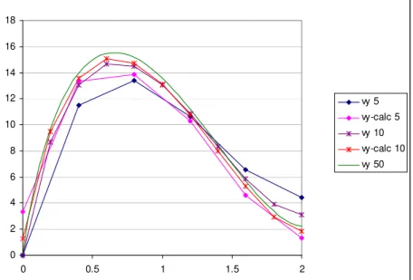
verified directly on ANSYS fluid element FLUID 141, where pressure and velocity components are nodal variables. Two test problems for unit viscosity and mass free fluid are specified in Fig. 6, results of original and recalculated normal velocities are shown in Figs. 7 and 8, respectively. No units are stated in the test problems, because only relative comparison is important. Moreover pressure in these test problems does not correspond to the capillary pressure, because the aim is only to test the efficiency of such methodology. Also here meshes of quad elements were used, now as 5x5, 10x10 and 50x50. The 50x50 mesh results can be assumed as the “exact” solution. In the legend of Figs. 7 and 8 original values of normal velocities are designated as “vy 5“, “vy 10“ and “vy 50“ on 5x5, 10x10 and 50x50 quad meshes, respectively, and the recalculated values are stated as “vy-calc 5“ and “vy-calc 10“.
Figure 7 - Results of the first test fluid problem.
Figure 8 - Results of the second test fluid problem.
It can be again verified that the recalculated outlet normal velocities on coarse meshes 5x5 and 10x10 fit the “exact” solution well.
-1500 -1000 -500 0 500 1000
0 0.5 1 1.5 2 vy 5
vy-calc 5 vy 10 vy-calc 10 vy 50
0 2 4 6 8 10 12 14 16 18
0 0.5 1 1.5 2
3.3 Mesolevel domain
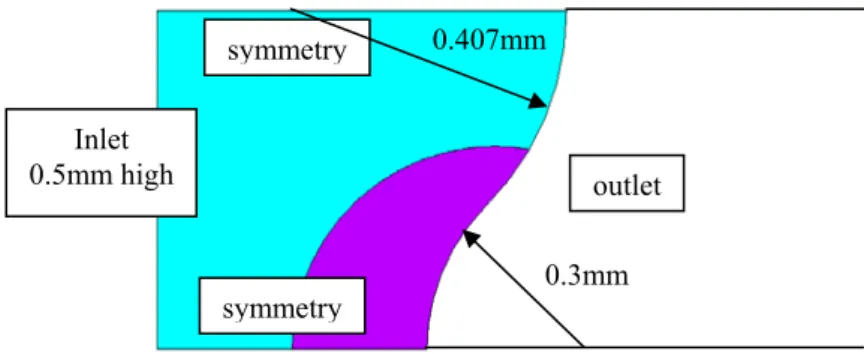
Flow domain with some intermediate free flow front was chosen according to Fig. 9. The outlet is thus composed from two parts of circumferences, as specified, in order to avoid errors which could be introduced due to the curvature approximation.
Figure 9 - Flow domain for the test problem at the mesolevel.
Resin properties were chosen as μ=0.05 Pa⋅s and γ=0.02N/m. At first only Stoke’s flow with inlet velocity 1mm/s was assumed (case 1) and then the violet part in Fig. 9 represented a fiber tow of radius 0.25mm with K=1.6·10-7mm2, tow porosity of 0.4, allowing the homogenized capillary pressure estimation as 1.9kPa. This arrangement was tested for inlet velocity 1mm/s (case 2) and 0.01mm/s (case3).
Figure 10 - Distribution of the element flux for the rough mesh in case 1.
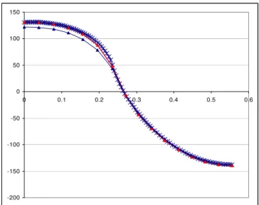
Fig. 10 shows the distribution of the element flux for a rough mesh. Results of the original and the recalculated outlet normal velocities are compared in Fig. 11 with the “exact” solution on very fine mesh. It is seen, that the error in element flux is concentrated around the outlet and that after the recalculation the outlet velocities fit well the fine mesh solution. Fig. 12 brings again the element flux, no for the fine mesh case. It is seen that there is still some element flux error left in the concave part of the outlet.
However, the results related to cases 2 and 3, shown in Fig. 13, clearly show the lack of some technique for the thin strip around the fiber tow surface, where viscous stress is important. This region still needs some further study.
symmetry
symmetry
outlet
0.3mm 0.407mm
Figure 11 – Original normal velocities for the rough mesh (blue line with triangles), recalculated normal velocities for the rough mesh (red line with triangles) and original normal
velocities for the fine mesh (blue line with crosses) in case 1 from bottom to top.
Figure 12 - Distribution of the element flux for the fine mesh in case 1.
Figure 13 – Original normal velocities for the rough mesh (blue line with triangles), recalculated normal velocities for the rough mesh (red line with triangles) and original normal
velocities for the fine mesh (blue line with crosses) in cases 2 (left) and 3(right), plotted from bottom to top.
-200 -150 -100 -50 0 50 100 150
0 0.1 0.2 0.3 0.4 0.5 0.6
0.0 0.5 1.0 1.5 2.0 2.5 3.0 3.5 4.0
0 0.1 0.2 0.3 0.4 0.5 0.6 -0.4
-0.2 0.0 0.2 0.4 0.6 0.8 1.0
4 CONCLUSION
It can be concluded that the stabilization techniques presented in this article are very efficient as shown in the simple test examples. They permit calculation of the frontal normal velocities with sufficient precision even for coarse meshes. They are now included in the post-processing part of FBP. Their implementation ensures better mass conservation at the global as well as the local level. It makes it possible to obtain a front shape that is not only more exact but also smoother. The computational time is reduced as coarser meshes can be used to obtain stable and accurate answers and it also allows one to step through larger time steps during the impregnation process.
Acknowledgments
Firstly named author would like to thank to the Portuguese institution for founding research Fundação para a Ciência e a Tecnologia for the scholarship allowing developing this work.
REFERENCES
Advani, S. G., Bruschke, M. V. & Parnas, R. S., 1994.Resin transfer molding. In Advani, S. G., ed, Flow and rheology in polymeric composites manufacturing, pp. 465-516, Elsevier Publishers, Amsterdam.
Advani, S. G. & Dimitrovová, Z., 2004. Role of capillary driven flow in composite manufacturing. In Hartland, S. ed, Surface and Interfacial Tension; Measurement, Theory and Application, Surfactant Science Series, vol. 119, pp. 263-312, Marcel Dekker, Inc., New York.
Babuška, I. & Miller, A., 1984. The post-processing approach in the finite element method - Part 1: Calculation of displacements, stresses and other higher derivatives of the displacements. International Journal for Numerical Methods in Engineering, vol. 20, pp. 1085-1109.
Binetruy, C., Hilaire, B. & Pabiot, J., 2000. The influence of fiber wetting in resin transfer molding: scale effects. Polymer Composites, vol. 24, pp. 548-557.
Dimitrovová, Z. & Advani, S. G., 2003. Free boundary viscous flows at micro and mesolevel during liquid composites molding process, in CD of communications of the 14th International Conference on Composites Materials (ICCM-14), San Diego, California, EUA.
Dimitrovová, Z. & Advani, S. G., 2004a. Free boundary viscous flows at micro and mesolevel during liquid composites molding process. International Journal for Numerical Methods in Fluids, vol. 46.
Hughes, T. J. R., Engel, G., Mazzei, L. & Larson, M. G., 2000. The continuous Galerkin method is locally conservative. Journal of Computational Physics, vol. 163, pp. 467-488.
Parnas, R. S. & Phelan, F. R., 1991. The effect of heterogeneous porous media on mold filling in resin transfer molding. SAMPE Quarterly, vol. 22, pp. 53-60.
Parnas, R. S., Salem, A. J., Sadiq, T. A. K., Wang, H. P. & Advani, S. G., 1994. The interaction between micro- and macroscopic flow in RTM preforms. Composite Structures, vol. 27, pp. 93-107.
Patel, N. & Lee, L. J., 1995. Effects of fiber mat architecture on void formation and removal in liquid composite molding. Polymer Composites, vol. 16, pp. 386-399.
Patel, N., Rohatgi, V. & Lee, L. J., 1995. Micro scale flow behavior and void formation mechanism during impregnation through a unidirectional stitched fiberglass mat. Polymer Engineering and Science, vol. 35, pp. 837-851.
Potter, K., 1997. Resin transfer molding. Chapman & Hall, London.
Sadiq, T. A. K., Advani, S. G. & Parnas, R. S., 1995. Experimental investigation of transverse flow through aligned cylinders. International Journal of Multiphase Flow, vol. 21, pp. 755-774.