Risk aversion, the disposition effect and decision-making in groups
Wlademir R. Pratesa, Newton C. A. da Costa Jr.b, Anderson Dorowc
a Doutorando em Administração, Departamento de Administração, Universidade Federal de Santa Catarina. E-mail: [email protected]
b Professor Doutor, Departamento de Economia, Universidade Federal de Santa Catarina. E-mail: [email protected] c Doutorando em Administração, Departamento de Administração, Universidade Federal de Santa Catarina. E-mail: [email protected]
2
Risk aversion, the disposition effect and decision-making in groups
Resumo
Este artigo apresenta os resultados de um experimento de laboratório conduzido com o propósito de investigar a forma
pela qual o efeito disposição afeta a decisão de investimento de indivíduos e grupos. Foram realizadas seis sessões
experimentais com 174 estudantes de graduação. Os estudantes exibiram o efeito disposição enquanto decidiam
sozinhos, porém o efeito deixou de ser estatisticamente significativo quando as decisões foram tomadas por grupos de
dois ou de três indivíduos. Também foi possível observar que o efeito disposição foi resultado de uma alta proporção de
ganhos realizados, indicando que os indivíduos foram mais avessos ao risco do que os grupos.
Palavras-chave: Efeito disposição, Aversão ao risco, Decisões em grupos.
Abstract
This paper presents the results of a laboratory experiment conducted to investigate the manner in which the disposition
effect affects individuals’ and groups’ investment decision making. We conducted six experimental sessions with 174 undergraduate students. We found that the students exhibited the disposition effect when working alone, but that the
effect was no longer statistically significant when they made decisions together in two and three-member groups. We
also observed that the disposition effect was the result of a high proportion of gains being realized, indicating that the
individuals were more risk averse than the groups.
Keywords: Disposition effect, Risk aversion, Group decisions. JEL Code: C91, C92, G02, G11
1 Introduction
Do groups take better decisions under risk than individuals? This article presents an analysis of how groups of
people behave when taking decisions under risk, with reference to the behavioral bias known as the disposition effect.
The disposition phenomenon is considered an anomaly in the standard behavior of financial agents and is
manifest in their reluctance to realize losses. Within the stock market, for example, people tend to hold stocks that have
lost value compared to their acquisition price longer than stocks that have gained value since purchase (Schlarbaum et
al. 1978; Shefrin and Statman 1985; Odean, 1998).
This behavior has been observed in several different contexts within finance and economics, including among
holders of stock options (Heath, Huddart and Lang, 1999), futures traders (Locke and Mann, 2005 and Coval and
3
students being studied in experimental economics laboratories (Myagkov and Plott,1997; Weber and Camerer, 1998; Da
Costa Jr. et al., 2008) and even among institutional investors (Grinblatt and Keloharju, 2001; Shapira and Venezia,
2001).
The inspiration for this article comes from Cooper and Kagel’s observation (2005, p. 478) that the majority of investment decisions taken in the financial market and also the strategic decisions taken within firms are the result of a
consensus reached between two or more people. This insight contrasts with the greater part of financial and economic
theories and their respective empirical tests, since they do not differentiate between decisions taken by groups and those
taken by individuals.
Some researchers are beginning to analyze the predictions made by theory with relation to the behavior of
groups, including scholars working in areas such as international relations (Levy, 1997), game theory (Kocher and
Sutter, 2005; Bornstein and Yaniv, 1998), strategy (Cooper and Kagel, 2005), and decision making under risk
(Rockenbach et al., 2007; Shupp and Williams, 2008),.
One theory that has been used to attempt to explain the disposition effect phenomenon is Prospect Theory,
which was developed by Kahneman and Tversky (1979). At this point it is important to point out that, while this article
draws on prospect theory, it does not aim to propose technical enhancements to the theory that would increase its
compatibility with the behavior of groups, even though it was originally developed on the basis of observation of the
behavior of individual people when faced with choices under risk (Kahneman and Tversky, 1979). To do so would
demand a high degree of mathematical complexity to deal with non-linear probability weighting functions, for example,
not to mention many other problems. The objective here is simply to attempt to detect differences between individual
and group behavior. It may be hoped that such findings and observations could in turn provide a basis for a technical
enhancement of prospect theory that would allow it to predict the behavior of people in aggregated terms, thereby
making it more realistic. Among others, Fiegenbaum and Thomas (1988), Whyte (1993) and Levy (1997) have applied
prospect theory to the study of group behavior, with reference to organizational behavior, sunk costs and international
relations, respectively.
This paper attempts to answer the following questions: (a) Can the disposition effect be detected in groups of
people tested under controlled laboratory conditions? (b) Is this effect different (greater or smaller) when the experiment
is conducted with individuals? (c) Does the effect change as the size of the group is increased?
The remainder of this paper is structured as follows. The next section presents the theoretical framework, the
third section describes the methodology employed, the fourth section presents and discusses the results and the last
4
2 Prospect theory, the disposition effect and group decision making
According to Thaler (1999, p.12), modern economic and financial theory is based on the assumption that the
“representative” economic agent takes decisions as predicted by expected utility theory and takes unbiased decisions with relation to the future. Those who defend this paradigm argue that the theory is not invalidated by the fact that some
people take sub-optimal, irrational decisions, as long as the marginal investor is rational. Irrational decisions end up
canceling each other out.
These concepts were considered to be robust, with the result that the study of stock market investor behavior
was not considered an attractive research avenue. Financial and economic research was therefore more concerned with
studying the behavior of prices. Notwithstanding, studies undertaken to investigate anomalies in the financial markets
found evidence of inconsistencies in decision-makers' reasoning, making it clear that there was a need to understand
other models of human behavior, such as those studied in the social sciences. Of particular interest among such models
is work published by the Israeli psychologists Amos Tversky and Daniel Kahneman.
2.1 Prospect theory
Kahneman and Tversky (1979) developed a descriptive theory called prospect theory on the basis of the results
of a series of laboratory experiments. This theory challenges the basics axioms of von Neumann and Morgenstern’s (1944) utility theory. One of the most important elements of Kahneman and Tversky’s work (1979, p.268) is a
description of an experiment conducted with students at three different universities (in Israel, the United States and
Sweden), showing that the decisions individuals take with regard to losses are an inverse reflection of the choices they
make with regard to gains. This experiment can be described as follows.
Suppose that a person is required to choose between the options available in the following prospect1:
(1) 80% chance of $4 thousand return and 20% of zero return; or
(2) 100% chance of $3 thousand return.
The prospect above is normally shown in the following compact form:
Option 1: ($4,000, 80%; $0, 20%) or Option 2: ($3,000, 100%)
Although the expected return from the risky option is higher (at $3.2 thousand), 80% of the people who took
part in the experiment chose the guaranteed three thousand.
1
According toKahneman and Tversky (1979), a prospect (or gamble) is a contract that yields result 𝑥𝑖 with probability
𝑝𝑖, where 𝑝1+ 𝑝2+ ⋯ + 𝑝𝑛= 1. A prospect offering “n” possible choices can therefore be shown as (𝑥1, 𝑝1; 𝑥2, 𝑝2 ; . .
5
Kahneman and Tversky (1979) then offered a different prospect to another sample of people. This time 92% of
the interviewees chose the riskier option (option 1), even though the expected loss of $3.2 thousand was greater than the
sure loss of $3 thousand. This prospect can be shown as follows:
Option 1: (-$4,000, 80%; $0, 20%) or Option 2: (-$3,000, 100%)
Kahneman and Tversky (1979), in common with many other researchers (Allais, 1953, Ellsberg, 1961,
Machina, 1982, Fishburn, 1982, and others), found that this asymmetrical pattern appears systematically across a wide
variety of experiments. While understandable, this behavior is incompatible with the assumptions of rational behavior
defended by expected utility theory, which is itself one of the pillars of neoclassical economics and of modern finance.
2.2 Risk aversion and the disposition effect
Tversky and Kahneman (1991) observed that there is strong evidence to be found in people’s behavior to
support the existence of a loss aversion phenomenon. They found that variation in the price of an asset has a greater
impact when the variation is seen as a loss than when the same degree of variation is seen as a gain; in other words
“losses loom larger than gains”.
In order to try to explain the apparently irrational behavior of people when faced with prospects such as those
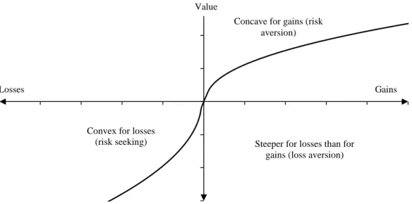
described above, Kahneman and Tversky (1979) proposed a value function (shown in Figure 1). There are two other
characteristics, in addition to loss aversion, that are essential to determining the asymmetrical “S” shape described by this function: the first is its “reference dependence”, meaning that the curve is centralized around a reference point, and the second is the fact that the marginal value of both gains and losses reduce in line with magnitude, indicating
“diminishing sensitivity”.
Figure 1. The prospect theory value function
Value
Gains Losses
Concave for gains (risk aversion)
Steeper for losses than for gains (loss aversion) Convex for losses
6
According to Shefrin and Statman (1985, p.779), the disposition effect becomes apparent when several factors
are present in combination. First, decision-makers (investors, in this case) make their choices in a very specific manner
(Kahneman and Tversky [1979] have labeled this the editing phase). During this phase, decision makers formulate all
possible choices in terms of gains and losses, with relation to a fixed reference point. During the second phase, called
the evaluation phase, decision makers use a value function (shown in Figure 1). This function is concave in the gain
region and convex in the loss region, reflecting risk aversion in the gain region and a propensity towards risk in the loss
domain. The characteristic loss aversion is shown by the steeper curve on the loss side, compared with the gain side.
An example adapted from Shefrin and Statman (1985, p.779) and Weber and Camerer (1998, p.170) provides a
good illustration of why the disposition effect is a consequences of loss aversion. Consider an investor who bought a
given stock at a certain time in the past when the price was $100 and now finds that it is trading at $80. This investor
must now decide whether to realize the loss or to continue holding the stock for a further period of time. To keep the
example simple, assume there are no taxes or transaction costs. Additionally, assume that there are two possible results
that may occur during the next period: either a $20 rise in the share price or a $20 fall, both with the same probability of
taking place. According to prospect theory, such an investor would make choices on the basis of the following prospect,
or gamble:
A - sell the stock now, thereby realizing what would be a loss of $20.
B - hold the stock for one more period, with a 50% chance of losing a further $20 and a 50% chance of gaining
$20, thereby recovering what has been lost previously.
Since the choice between the two possible results of this prospect is within the convex part of the "S" shaped
value function, prospect theory predicts that option B will be chosen rather than option A. In other words, the investor
will choose the risky option and hold the losing stock. An analogous argument can be used to show that, according to
prospect theory, the same investor would choose to sell the stock if this involved a gain.
2.3 Groups
The literature on the decision-making behavior of groups and individuals within financial contexts is still
recent and because of this there is not yet consensus on whether groups take better decisions than individuals.2 Some
studies have found evidence for the superiority of groups (Blinder and Morgan, 2005; Rockenbach et al., 2007), and
others for the superiority of individuals (Whyte, 1993; Kocher and Sutter, 2005), while yet others have reported
indefinite results (Bone et al., 1999; Shupp and Williams, 2008). Studies have also been conducted to investigate factors
2 In general, a group is formed when two or more people work together to accomplish a common task. In psychology, a small group is made up of no more than 15 members and normally would not pass 10 (Tuckman,1965). Slater (1955), for example, considered small groups to have from three to seven members.
7
other than the number of members in decision-making groups, such as for example, whether differences can be linked to
sex, educational level or the location (country) in which the research subjects live.
Blinder and Morgan (2005) attempted to determine whether groups of five people performed better than
individuals, analyzing decision-making in two different experiments: the first dealt with questions of monetary policy
while the second was a purely statistical task. When analyzing their results, Blinder and Morgan (2005) found that in
the first experiment (monetary policy) groups were superior to individuals by 3.5 percentage points, while in the second
experiment (urns) groups were superior to individuals by 3.7 percentage points. The authors therefore concluded that
groups performed better than individuals in both experiments and also noted that they did not take any longer than
individuals to arrive at their decisions.
Kocher and Sutter (2005) conducted an experiment using a “beauty-contest game” designed to determine whether there are differences in terms of reasoning, learning and efficiency when decisions are taken by individuals or
by groups of three people. They found that, as the game was repeated, groups exhibited a greater capacity to learn the
game’s dynamics and achieve better results.
Kugler et al. (2007) studied a game in which players were either groups of three people or individuals and
which was designed to identify the level of trust in decision making. The game involved two players: (i) a sender and
(ii) a responder. The sender is given an endowment and may send any fraction to the responder. The sum sent is tripled
and the responder may send any fraction of the tripled amount back to the sender. The authors found that when groups
were playing as senders, they normally exhibited less trust than individuals, but they found no difference between the
returns sent by groups and by individuals.
Sutter (2005) investigated the decision-making process in groups of four and of two members and compared
the results with those for individuals. The size of the groups was varied in attempt to supplement work by Kocher and
Sutter (2005), in which groups had achieved higher returns than individuals, but which had not varied the number of
group members.
In common with the study by Kocher and Sutter (2005), the study Sutter (2005) conducted also used the beauty-contest
game. He found that groups with four members were superior to individuals but that two-member groups did not
perform significantly differently from individuals. On this basis, he claimed that group size is a relevant variable for
determining team performance.
Bornstein and Yaniv (1998) analyzed decision-making under risk by groups and individuals using a game
called ultimatum. In this game there are two players who must interact to decide how to divide a sum of money that has
been given to them. Player A makes the offer, proposing how the sum will be divided between the two players. Player B
8
money. If B accepts the offer, then the sum will be duly divided as proposed by A. Additionally, the game is only played
once. Bornstein and Yaniv (1998) analyzed the results for 20 groups of three people (30 player As and 30 player Bs) and
for 20 individual players (10 player As and 10 player Bs). They found that groups behaved more rationally that
individual decision makers, because they offered less when they were playing the A role and demanded less when they
were in the player B receiving role, thereby demonstrating better understanding of the game’s structure, particularly when playing the offering role (player A).
Bone et al. (1999) tested the consistency of group decision-making against individual decision-making using a
game called Common-Ratio. Players analyzed 12 probabilities during three stages of the game, playing stages one and
three individually and stage two in groups. In this case there was little evidence that the groups were more consistent
than individuals. Notwithstanding, the authors noted that having participated in groups helped individuals to increase
their consistency of reasoning in the final stage of the game. They therefore concluded that individuals achieved better
results after having participated in a group decision-making stage, acquiring improved rational consistency.
Rockenbach et al. (2007) published an article specifically related to risk in finance, analyzing groups’ behavior under risk on the basis of expected utility theory and portfolio selection theory. These authors did not find evidence that
groups and individuals behaved differently with relation to expected utility theory, but they did find substantial
differences in consistency with relation to portfolio theory. Groups performed better than individuals in terms of
risk-adjusted returns. Rockenbach et al. (2007) considered that the groups’ advantage lay in avoiding excessive exposure to risk, which individuals often failed to avoid.
Shupp and Williams (2008) found that, on average, groups are more risk-averse in high-risk situations. In
contrast, groups behave with less risk-aversion in low-risk situations.
3 Methodology
3.1 Experimental design and ExpEcon software
The experiments were conducted with undergraduate students who took investment decisions using software
called ExpEcon, designed to simulate a simplified share market (Goulart et al., 2008).
ExpEcon was developed with reference to an experiment described by Weber and Camerer (1998) that
involved dealing in six shares over 14 simulation periods. It should be noted that both Weber and Camerer’s
experiments (1998) and the ExpEcon software simulate an exogenous market in which prices are preset and are not
affected by the buying and selling decisions of the game’s participants.
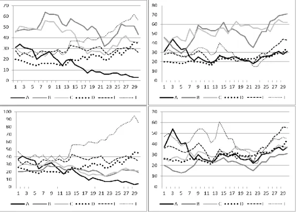
The database used for the experiments was sub-sampled to provide four different configurations. Each
9
prices were based on the monthly variation in the prices of the most liquid stocks in the São Paulo stock market’s index
(the IBOVESPA index) and each configuration covered a 30-month period selected at random from the interval 2000 to
2010. Figure 2 illustrates the four configurations utilized.
Three different experimental designs were used, with players varying as follows: (i) individuals; (ii) groups of
two people; (iii) groups of three people. The experimental participants were 174 undergraduate students studying for
degrees in Management, Accounting, Economic Science or International Relations at the Universidade Federal de Santa
Catarina. This sample was divided as follows: 30 individuals, 30 pairs and 28 groups of three. Data were collected in six
experimental sessions.
A system for rewarding participants was included in order to the increase internal validity of the experimental
sessions.3 At the end of each session those participants (whether playing individually or in groups) whose results were
in the top quartile in terms of payoff were entered into a draw to win a prize. The prize awarded was calculated as
follows: each player began the simulation with 10,000 monetary units at their disposal; when the winning group or
individual was drawn, their final number of monetary units (payoff) was divided by 1000 and each member of the group
was paid that number of Reais. For example, if a three-member group was drawn and had a payoff of 15,000 monetary
units, then each member would receive a total of R$ 15.00, making R$ 45.00 prize money for the whole group.
Figure 2. The four simulation configurations
3 For a discussion of the importance of employing reward mechanisms in experiments see Smith (1976) and Friedman and Cassar (2004).
10
3.2 Estimating the disposition effectThe methodology used to measure the disposition effect was based on Odean (1998). An individual or group
was considered to exhibit the disposition effect if their Proportion of Gains Realized (PGR) was greater than their
Proportion of Losses Realized (PLR) over the period analyzed. The result of subtracting PLR from PGR was termed the
Disposition Coefficient (DC). A positive DC indicates the presence of the disposition effect, since it shows that the
investor has realized a higher percentage of gains than losses. The variables described above are now presented below:
RG𝑖
RG𝑖+ PGi= PRG 𝑖 (1)
RLi
Rli+ PLi = PRL𝑖 (2)
DC𝑖= PRG𝑖− PRL𝑖 (3)
where, RG represents realized gains, PG stands for paper gains, which are unrealized or potential gains, PGR is the
proportion of realized gains, RL is realized losses, PL is paper losses, PLR the proportion of realized losses, DC is the
disposition coefficient and i the individual or group investor.
The Disposition Coefficient is generally given in two forms: (i) individual and (ii) aggregated. In the first case,
DC is calculated for each experimental unit. In the second, an overall DC is calculated for each treatment. Since the
results for both methods were similar, we chose to present only the individual data. The aggregate data is shown in
Appendix A.
As shown by Kahneman and Tversky (1979), it is necessary to calculate a reference point before gains and
losses can be estimated (RG and RL). The reference point used here was the Average Purchase Price. There are other
methods for calculating a reference point, such as the highest purchase price, the first purchase price or the latest
purchase price. However, we chose to follow Odean (1998) and Weber and Camerer (1998) in using the average
purchase price.
The average purchase price was calculated by dividing the cost of the shares bought by the number of shares in
the portfolio. Each time an individual or group bought additional quantities of a stock that they already held in their
portfolio, their average purchase price was weighted using the initial purchase price and each subsequent purchase
11
price; and a sale operation was considered a loss if the price obtained was lower than the average purchase price.
After the proportions of realized gains and losses had been obtained, the disposition coefficient was calculated
(Equation 3) for each experimental unit (individuals, pairs and three-member groups). In order to verify whether the
disposition coefficient really exists from a statistical point of view, two possibilities can be tested: (i) 𝐻0: 𝐷𝐶 = 0 and
𝐻1: 𝐷𝐶 > 0; (ii) 𝐻0: 𝑃𝑅𝐺 = 𝑃𝑅𝐿 and 𝐻1: 𝑃𝑅𝐺 > 𝑃𝑅𝐿. Tests of these two hypotheses were therefore conducted for both
means (t test) and medians (Wilcoxon signed rank test and Mann-Whitney U-test). (Wilcoxon, 1945; Mann and
Whitney, 1947).
After testing the significance of the results of tests conducted up to this point, we attempted to verify whether
DC, PGR or PLR differed across treatments. To achieve this, we first conducted simple linear regression for which
dependent variables were DC, PGR and PLR; and the independent variable was a dummy variable for groups (including
pairs and three-member groups in the same variable), as shown in Equation 44:
𝑦𝑖= 𝛼 + 𝐺𝑅𝑂𝑈𝑃𝑆𝑖+ 𝜀𝑖 (4)
where 𝑌𝑖 can be DC (disposition coefficient), PGR (Proportion of Gains Realized) or PLR (Proportion of Losses
Realized); 𝐺𝑅𝑂𝑈𝑃𝑆𝑖 is a dummy variable that takes 𝐺𝑅𝑂𝑈𝑃𝑆𝑖= 1 for groups (with two or three members), and
𝐺𝑅𝑂𝑈𝑃𝑆𝑖= 0 for individuals.
We also conducted a multivariate regression that differs from Equation (4) in that two dummies were included,
one to indicate two-member groups and the other for three-member teams, as shown below:
𝑦𝑖= 𝛼 + 1𝑃𝐴𝐼𝑅𝑆𝑖+ 2𝑇𝑅𝐼𝑂𝑆𝑖+ 𝜀𝑖 (5)
where 𝑌𝑖 can be DC, PGR or PLR; 𝑃𝐴𝐼𝑅𝑆𝑖 is a dummy to indicate whether the group is a pair (1 if a pair, 0 if not);
𝑇𝑅𝐼𝑂𝑆𝑖 is a dummy to indicate whether the group is a three-member group (1 if a three-member group, 0 if not).
3.3 Simulations with robots
In addition to the analyses of the results from the experimental sessions, we also conducted a number of
randomized simulations on the ExpEcon software. The simulations followed the following rules: (i) the database
configuration to be used (from the four shown in Figure 2) was chosen at random for each simulation; (ii) the trade
(whether purchase or sale) and the stock to be traded were selected at random; and (iii) the value of each trade was also
4
12
selected at random. For each buy trade a random percentage of the amount of monetary units held at that point was
generated. If a sale was chosen, then the percentage of stock sold was randomized from the total number of shares of the
stock to be traded that were held at that point. Sales of assets that had not yet been bought were ignored. Thirty
simulations were run in this manner.
The purpose of conducting these simulations was to make it possible to compare the results obtained with each
of the three treatments tested experimentally (decisions taken by individuals, by two people or by three people) with
results obtained from entirely unbiased decision-making, i.e., decisions taken at random. These data were analyzed
using the same methodology adopted for the data obtained from the experiments with the students.
4 Results
This section presents the study results. Table 1 lists some of the statistics for the data from the simulations
using ExpEcon. It can be observed that mean returns were greatest among three-member groups and that, curiously, the
mean number of trades conducted during experiments was the same for individuals as for groups. Table 1 also shows
that individuals generally held more diversified portfolios than groups.
As was explained in the methodology section, the disposition effect can be measured either as an aggregated
figure (calculating a single disposition coefficient for each sample based on the sum of realized gains and losses) or as
an individual figure (calculating one disposition coefficient for each sample unit, thereby obtaining several coefficients
and making it possible to conduct statistical tests for differences between means and medians, for example). In this
section, only the results for the individual level are shown. The aggregated results are given in Appendix A.
Table 1. General statistics
Overall Results Individuals Pairs Three
People Robots
Observations 88 30 30 28 30
Mean return 31.7% 28.9% 24.6% 42.2% 16.5%
Mean number of trades 42 42 42 42 28
Total number of trades 3703 1251 1265 1187 834
Mean number of stocks in
portfolio per period 3.3 2.8 3.7 3.5 3.7
Note: The overall results columns in this table and the next do not include the data from the robots, only from the individuals, pairs and three-member teams.
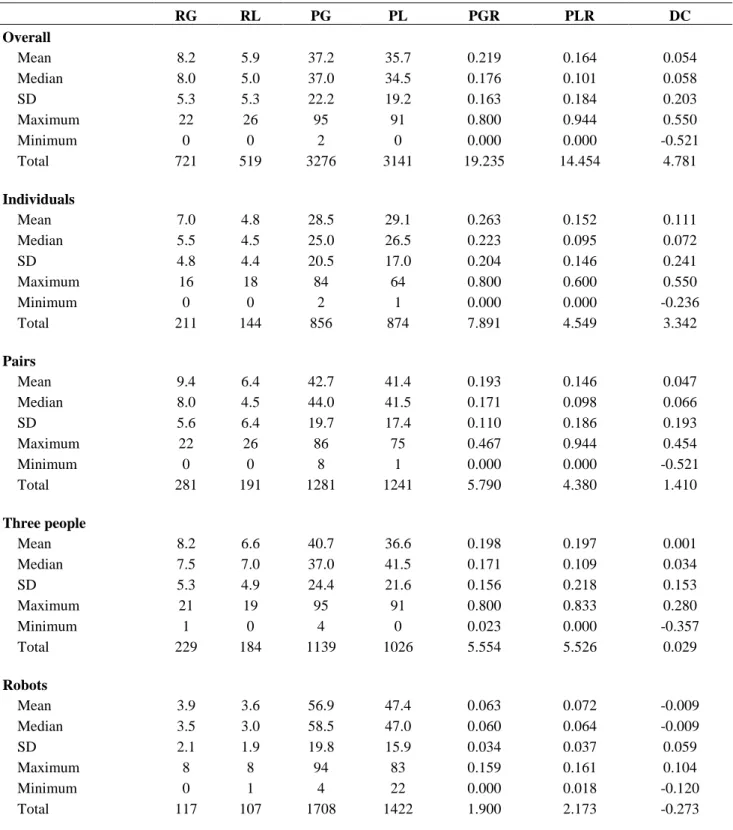
Table 2 contains descriptive statistics for the data. With the exception of the random simulations (robots),
means and medians for Proportion of Gains Realized (PGR) were always higher than the means and medians for
Proportion of Losses Realized (PLR). This meant that there were positive Disposition Coefficients for all three
13
Table 2. Descriptive statistics
RG RL PG PL PGR PLR DC Overall Mean 8.2 5.9 37.2 35.7 0.219 0.164 0.054 Median 8.0 5.0 37.0 34.5 0.176 0.101 0.058 SD 5.3 5.3 22.2 19.2 0.163 0.184 0.203 Maximum 22 26 95 91 0.800 0.944 0.550 Minimum 0 0 2 0 0.000 0.000 -0.521 Total 721 519 3276 3141 19.235 14.454 4.781 Individuals Mean 7.0 4.8 28.5 29.1 0.263 0.152 0.111 Median 5.5 4.5 25.0 26.5 0.223 0.095 0.072 SD 4.8 4.4 20.5 17.0 0.204 0.146 0.241 Maximum 16 18 84 64 0.800 0.600 0.550 Minimum 0 0 2 1 0.000 0.000 -0.236 Total 211 144 856 874 7.891 4.549 3.342 Pairs Mean 9.4 6.4 42.7 41.4 0.193 0.146 0.047 Median 8.0 4.5 44.0 41.5 0.171 0.098 0.066 SD 5.6 6.4 19.7 17.4 0.110 0.186 0.193 Maximum 22 26 86 75 0.467 0.944 0.454 Minimum 0 0 8 1 0.000 0.000 -0.521 Total 281 191 1281 1241 5.790 4.380 1.410 Three people Mean 8.2 6.6 40.7 36.6 0.198 0.197 0.001 Median 7.5 7.0 37.0 41.5 0.171 0.109 0.034 SD 5.3 4.9 24.4 21.6 0.156 0.218 0.153 Maximum 21 19 95 91 0.800 0.833 0.280 Minimum 1 0 4 0 0.023 0.000 -0.357 Total 229 184 1139 1026 5.554 5.526 0.029 Robots Mean 3.9 3.6 56.9 47.4 0.063 0.072 -0.009 Median 3.5 3.0 58.5 47.0 0.060 0.064 -0.009 SD 2.1 1.9 19.8 15.9 0.034 0.037 0.059 Maximum 8 8 94 83 0.159 0.161 0.104 Minimum 0 1 4 22 0.000 0.018 -0.120 Total 117 107 1708 1422 1.900 2.173 -0.273
Notes: Presentation of data, where RG is realized gains, RL realized losses, PG is paper gains, PL is paper losses, PGR and PLR are
proportions of realized gains and losses and DC is the disposition coefficient. The values shown (mean, median, standard deviation, maximum, minimum and totals) relate to data in the individual (non-aggregated) format, used to calculate the Disposition Coefficients and for the statistical tests.
While not shown in the tables, the Jarque-Bera and Anderson-Darling tests of normality were applied to DC
distributions. In no case was the null hypothesis, that the variable’s distribution was normal, rejected (p-value < 0.10). However, the same tests were used for PGR and PLR and the results did indicate rejection of the null hypothesis of
14
are more robust for the case 𝐻1: 𝐷𝐶 > 0 than for the proportions of gains and losses (𝐻1: 𝑃𝑅𝐺 > 𝑃𝑅𝐿). Table 3 also
lists the results for the Wilcoxon and Mann-Whitney tests, which are nonparametric and do not therefore demand
normal distribution.
The t test of means for the hypothesis 𝐻1: 𝐷𝐶 > 0 was statistically significant for overall results, for
individuals and for pairs (individuals: p-value < 0.01; pairs: p-value < 0.10). For 𝐻1: 𝑃𝑅𝐺 > 𝑃𝑅𝐿, 𝐻0 was rejected for
overall results and for individuals, with p-values of < 0.05 and < 0.01, respectively. Tests of means did not achieve
statistical significance for the three-member groups.
The result of the tests of medians is similar to those for the means. The Wilcoxon test results for one sample
(𝐻1: 𝐷𝐶 > 0) indicate statistical significance for individuals (p-value < 0.05), for pairs (p-value < 0.05) and for overall
results (p-value < 0.01). The Mann-Whitney test also detected statistical significance for individuals (p-value < 0.05),
for pairs (p-value < 0.01) and for overall results (p-value < 0.01). In common with the means, the tests of medians did
not return statistically significant results for three-member groups.
The results obtained from the randomized simulations with robots, shown in Table 3, did not achieve statistical
significance for any of the tests conducted. In other words, the randomized simulations were free from the disposition
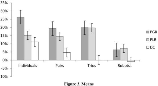
effect bias (PGR and PLR were both similar and statistically indistinguishable). Figures 3 and 4 illustrate this situation.
Table 3. Disposition Coefficients (calculated at the individual level)
Overall
Results Individuals Pairs
Three People Robots Observations 88 30 30 28 30 Tests t test (𝐻1: 𝐷𝐶 > 0) 2.49*** 2.51*** 1.31* 0.04 -0.84 teste t (𝐻1: 𝑃𝑅𝐺 > 𝑃𝑅𝐿) 2.08** 2.46*** 1.19 0.01 -0.98 Wilcoxon (𝐻1: 𝐷𝐶 > 0) 2482*** 310** 315** 222 189 Mann-Whitney (𝐻1: 𝑃𝑅𝐺 > 𝑃𝑅𝐿) 8912*** 1060** 1093*** 872 854
15
Figure 3. MeansFigure 5 illustrates the empirical Cumulative Distribution Function for the Disposition Coefficients, based on a
normal distribution. This function is appropriate since H0 was accepted in the Jarque-Bera and Anderson-Darling tests
of normality. Figures 3, 4 and 5 show that DC reduces gradually as the number of group members increases.
Furthermore, this difference in DC between treatments appears to be greater in the gains zone (when the Proportion of
Gains Realized is greater than the Proportion of Losses Realized, i.e. 𝐷𝐶 > 0) than it is in the losses zone (DC< 0).
Figure 4. Medians -10% -5% 0% 5% 10% 15% 20% 25% 30% 35%
Individuals Pairs Trios Robots
PGR PLR DC -5% 0% 5% 10% 15% 20% 25% 30%
Individuals Pairs Trios Robots
PGR PLR DC
16
0.75 0.50 0.25 0.00 -0.25 -0.50 100 80 60 40 20 0 Disposition Coefficient % Individuals Pairs Three-member RobotsFigure 5. Empirical cumulative distribution
Observing the means and medians for PGR and PLR in Table 2 and Figures 3 and 4, it will be noted that PGR
for individuals was greater than for both sizes of group (pairs and three-member groups). It can also be observed from
Table 2 and Figures 3 and 4 that PLR was greater for three-member groups than for individuals or for pairs. Simple
linear regression and then multivariate linear regression with dummy variables were conducted in order to test whether
these differences were statistically significant. These regressions are described by Equations 4 and 5and their results are
shown in Tables 4 and 5, respectively.
Models (1) from Table 4 and (4) from Table 5 provide confirmation that the classification of decision makers
into groups or individuals reveals a difference in terms of the results for disposition coefficients, with lower coefficients
for groups (especially three-member groups) than for individuals. The second model from Table 4 shows that the lower
PGR for groups than for individuals was confirmed statistically by the regressions (𝐹 = 3.48, p-value < 0.10). The higher PGR for individuals than for groups may indicate that individuals are more risk averse, since they realize more
gains than the groups do. This difference is also apparent in Figures 3 and 4. Although significant differences were
detected for Proportions of Realized Gains (PGR), no significant differences were detected for Proportions of Realized
17
Table 4. Results of Equation 4
Dummy groups R² F Model Dependent variable Coefficient SE t (1) DC -0.087 0.042 -1.75* 0.042 3.72** (2) PGR -0.067 0.034 -1.65* 0.039 3.48* (3) PLR 0.019 0.033 0.51 0.02 0.21
Notes: The results shown in this table are derived from the equation: 𝑦𝑖= 𝛼 + 𝐺𝑅𝑂𝑈𝑃𝑆𝑖+ 𝜀𝑖, where 𝑦𝑖 takes the value of DC, PGR or PLR In turn, 𝐺𝑅𝑂𝑈𝑃𝑆𝑖 is a dummy variable for both sizes of group (1 for groups and 0 for individuals).
*Significant to 10% **Significant to 5% ***Significant to 1%
Table 5. Results of Equation 5
Model Dependent variable
Dummy pairs Dummy three-member groups
R² F Coeff. SE t Coeff. SE t (4) DC -0.064 0.049 -1.14 -0.110 0.043 -2.10** 0.050 2.24 (5) PGR -0.070 0.035 -1.65* -0.065 0.042 -1.36 0.039 1.73 (6) PLR -0.006 0.041 -0.13 0.046 0.037 0.93 0.015 0.66
Notes: The results shown in this table are derived from the equation: 𝑦𝑖= 𝛼 + 1𝑃𝐴𝐼𝑅𝑆𝑖+ 2𝑇𝑅𝐼𝑂𝑆𝑖+ 𝜀𝑖, where 𝑦𝑖 takes the value of DC, PGR or PLR In turn, 𝑃𝐴𝐼𝑅𝑆𝑖 and 𝑇𝑅𝐼𝑂𝑆𝑖 are dummy variables for pairs and three-member groups respectively (1 for pairs or three-member groups, as appropriate, and 0 for other cases).
*Significant to 10% **Significant to 5% ***Significant to 1%
Finally, as explained in the methodology section, experiments were conducted using four different database
configurations (see Figure 2) which were allocated to participants at random at the start of each experiment. In order to
test whether the disposition coefficient had been influenced by the initial simulation configuration selected, a one-factor
analysis of variance (ANOVA) was conducted with the whole-sample disposition coefficient as dependent variable and
the factor defined as a series from 1 to 4, to represent the different initial configurations used (𝐷𝐶𝑖,𝑗 = 𝐷𝐶𝑖+ 𝑡𝑗, where i
is the experimental unit and j represents the effect of the four treatments). The results did not reveal any statistical
significance (p-value = 0.43). In other words, the four initial configurations used for the experiments did not affect the
resulting disposition coefficients.
5 Final comments
The experimental sessions conducted for this study confirmed the presence of a disposition effect among the
individuals. However, the disposition effect appeared to become attenuated as more members were added to groups.
The analyses conducted were unable to statistically confirm the disposition effect for the three-member groups. Among
pairs, the effect was detectable but at a lower level than among the individual investors.
The results of this study with respect to individual decision makers confirm what has been observed by other
18
observed that groups did not exhibit the disposition effect and, furthermore, when the Proportion of Gains Realized
(PGR) and Proportion of Losses Realized (PLR) were analyzed, it was found that individuals had higher PGR than
groups, but that PLR did not differ statistically between groups and individuals. With respect to the sample described
here, it can therefore be stated that the disposition effect exhibited by the individual investors was the result of a greater
inclination to realize gains. Such behavior may be an indication that the individuals were more risk-averse than groups
when the prices of the shares they were holding in their portfolios were at highs. In contrast, the groups’ behavior was more uniform for both shares at highs and at lows, with relation to the average price of purchase (based on the
proximity of the proportions of gains and losses realized - PGR and PLR). In this respect, the groups’ behavior was
closer to what is expected according to traditional financial theories.
6 References
Allais, M., 1953. Le comportement de l’homme rationnel devant le risque: Critique des postulats et axiomes de l’école américaine. Econometrica 21 (4), 503–546.
Blinder, A., Morgan, J., 2005. Are two heads better than one? Monetary policy by committee. Journal of Money, Credit, and Banking 37 (5), 798–811.
Bone, J., Hey, J., Suckling, J., 1999. Are groups more (or less) consistent than individuals? Journal of Risk and Uncertainty 18 (1), 63–81.
Bornstein, G., Yaniv, I., 1998. Individual and group behavior in the ultimatum game: Are groups more “rational” players? Experimental Economics 1 (1), 101–108.
Cooper, D., Kagel, J., 2005. Are two heads better than one? Team versus individual play in signaling games. American Economic Review 95 (3), 477–509.
Coval, J., Shumway, T., 2005. Do behavioral biases affect prices? Journal of Finance 60 (1), 1–34.
Da Costa Jr, N., Mineto, C., Da Silva, S., 2008. Disposition effect and gender. Applied Economics Letters 15 (6), 411–416.
Ellsberg, D., 1961. Risk, ambiguity, and the savage axioms. Quarterly Journal of Economics 75 (4), 643–669. Fiegenbaum, A., Thomas, H., 1988. Attitudes toward risk and the risk-return paradox: Prospect theory explanations.
Academy of Management journal 31 (1), 85–106.
Fishburn, P., 1982. Nontransitive measurable utility. Journal of Mathematical Psychology 26 (1), 31–67. Friedman, D., Cassar, A., 2004. Economics Lab: An Introduction to Experimental Economics. Routledge.
Genesove, D., Mayer, C., 2001. Loss aversion and seller behavior: Evidence from the housing market. Quarterly Journal of Economics 116 (4), 1233–1260.
Goulart, M. A., Schmaedech, D., Costa Jr., N. C. A., 2008. ExpEcon: capital market simulation.URL http://cpga.ufsc.br/expecon/index.html.
Grinblatt, M., Keloharju, M., 2001. How distance, language, and culture influence stockholdings and trades. Journal of Finance 56 (3), 1053–1073.
Heath, C., Huddart, S., Lang, M., 1999. Psychological factors and stock option exercise. Quarterly Journal of Economics 114 (2), 601–627.
Kahneman, D., Tversky, A., 1979. Prospect theory: An analysis of decision under risk. Econometrica 47 (2), 263– 291.
Kerr, N., MacCoun, R., Kramer, G., 1996. Bias in judgment: Comparing individuals and groups. Psychological Review 103 (4), 687–719.
Kocher, M., Sutter, M., 2005. The decision maker matters: Individual versus group behaviour in experimental beauty-contest games. The Econo- mic Journal 115 (500), 200–223.
Kugler, T., Bornstein, G., Kocher, M., Sutter, M., 2007. Trust between individuals and groups: Groups are less trusting than individuals but just as trustworthy. Journal of Economic psychology 28 (6), 646–657.
19
Levy, J., 1997. Prospect theory, rational choice, and international relations. International Studies Quarterly 41 (1), 87– 112.
Locke, P., Mann, S., 2005. Professional trader discipline and trade disposition. Journal of Financial Economics 76 (2), 401–444.
Machina, M., 1982. Expected utility analysis without the independence axiom. Econometrica, 50 (2), 277–323. Mann, H. B., Whitney, D. R., 1947. On a test of whether one of two random variables is stochastically larger than the
other. Annals of Mathematical Statistics 18 (1), pp. 50–60.
Myagkov, M., Plott, C., 1997. Exchange economies and loss exposure: Experiments exploring prospect theory and competitive equilibria in market environments. American Economic Review, 87 (5), 801–828.
Odean, T., 1998. Are investors reluctant to realize their losses? Journal of Finance 53 (5), 1775–1798.
Rockenbach, B., Sadrieh, A., Mathauschek, B., 2007. Teams take the better risks. Journal of Economic Behavior & Organization 63 (3), 412–422.
Schlarbaum, G. G., Lewellen, W. G., Lease, R. C., 1978. Realized returns on common stock investments: The experience of individual investors. Journal of Business 51 (2), 299–325.
Shapira, Z., Venezia, I., 2001. Patterns of behavior of professionally managed and independent investors. Journal of Banking & Finance 25 (8), 1573–1587.
Shu, P. G., Yeh, Y. H., Yamada, T., 2002. The behavior of Taiwan mutual fund investors-performance and fund flows. Pacific-Basin Finance Journal 10, 583–600.
Shefrin, H., Statman, M., 1985. The disposition to sell winners too early and ride losers too long: Theory and evidence. Journal of Finance 40 (3), 777–790.
Shupp, R., Williams, A., 2008. Risk preference differentials of small groups and individuals. Economic Journal 118 (525), 258–283.
Slater, P., 1955. Role differentiation in small groups. American Sociological Review 20 (3), 300–310.
Smith, V., 1976. Experimental economics: Induced value theory. American Economic Review, 66 (2), 274–279. Sutter, M., 2005. Are four heads better than two? An experimental beauty-contest game with teams of different size.
Economics Letters 88 (1), 41–46.
Thaler, R., 1999. The end of behavioral finance. Financial Analysts Journal 55 (6), 12–17.
Tuckman, B., 1965. Developmental sequence in small groups. Psychological Bulletin 63 (6), 384–399.
Tversky, A., Kahneman, D., 1991. Loss aversion in riskless choice: A reference-dependent model. Quarterly Journal of Economics 106 (4), 1039–1061.
Von Neumann, J., Morgenstern, O., 1953. Theory of games and economic behavior, 3rd Edition. Princeton University Press, Princeton.
Weber, M., Camerer, C., 1998. The disposition effect in securities trading: An experimental analysis. Journal of Economic Behavior & Organization 33 (2), 167–184.
White, H., 1980. A heteroskedasticity-consistent covariance matrix estimator and a direct test for heteroskedasticity. Econometrica 48 (4), 817–838.
Whyte, G., 1993. Escalating commitment in individual and group decision making: A prospect theory approach. Organizational Behavior and Human Decision Processes 54 (3), 430–455.
20
Appendix AThis appendix contains the results of the aggregated analysis of the disposition coefficients. Here, rather than
calculating a DC value for each experimental unit, an aggregated DC was calculated for each of the three treatments
(individuals, pairs and three-member groups) and for the randomized simulations (robots). For each treatment, PGR was
compared with PLR to see if it was greater and, if so, the difference was tested for statistical significance. In view of
this, the Z test for differences between proportions is an appropriate method for illustrating the differences. The standard
error calculation used for the denominator of the equation shown below was adapted from Odean (1998, p. 1784) and
Shefrin and Statman (1985, p. 789):
𝑍𝑖= 𝑃𝐺𝑅𝑖− 𝑃𝐿𝑅𝑖 √𝑃𝐺𝑅𝑖(1 − 𝑃𝐺𝑅𝑖) (𝑅𝐺𝑖+ 𝑃𝐺𝑖) + 𝑃𝐿𝑅𝑖(1 − 𝑃𝐿𝑅𝑖) (𝑅𝐿𝑖+ 𝑃𝐿𝑖)
where, 𝑍𝑖 is the Z statistic for each treatment 𝑖. P-values can be obtained from tables of critical values for the Z statistic.
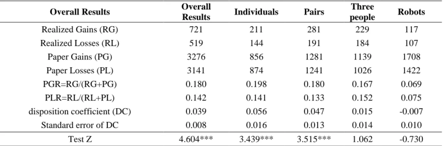
Table 6. Statistics for Disposition Coefficients at the aggregated level
Overall Results Overall
Results Individuals Pairs
Three people Robots Realized Gains (RG) 721 211 281 229 117 Realized Losses (RL) 519 144 191 184 107 Paper Gains (PG) 3276 856 1281 1139 1708 Paper Losses (PL) 3141 874 1241 1026 1422 PGR=RG/(RG+PG) 0.180 0.198 0.180 0.167 0.069 PLR=RL/(RL+PL) 0.142 0.141 0.133 0.152 0.075 disposition coefficient (DC) 0.039 0.056 0.047 0.015 -0.007 Standard error of DC 0.008 0.016 0.013 0.014 0.010 Test Z 4.604*** 3.439*** 3.515*** 1.062 -0.730
Notes: Overall results do not include the results for the robots, i.e. they only combine results from individuals, pairs and three-member groups.
*** Significant to 1% ** Significant to 5% * Significant to 10%
Table 6 lists the aggregated results, which are similar to those obtained at the individual level. It will be noted
that PGR is greater than PLR and that the difference is statistically significant for overall results, individuals and pairs.
While the results for pairs indicated a DC that is significant to 1%, it will be noted that the DC for pairs (0.047) was
lower than the DC for individuals (0.056). In other words, Table 6 reflects the same pattern that can be observed in
Figure 3, in that the DC for individuals is greater than the DC for pairs, which is in turn greater than the DC for the
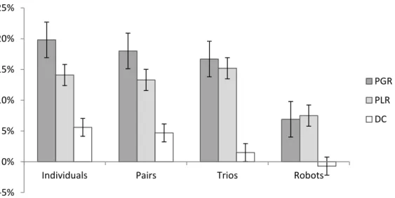
three-member groups. Figure 6 illustrates the aggregated data in the form of a graph, clearly showing how PGR falls
progressively from the first to the third treatment, indicating that groups realized fewer gains than individuals. Similar
21
Figure 6. Aggregated Data -5% 0% 5% 10% 15% 20% 25%
Individuals Pairs Trios Robots
PGR PLR DC