Velocity Field Analysis of a Channel Narrowed by Spur-dikes to Maximize Power Output of In-stream Turbines

(1)

Journal of Sustainable Development of Energy, Water and Environment Systems

http://www.sdewes.org/jsdewes

Year 2018, Volume 6, Issue 3, pp 534-546

534

Journal of Sustainable Development of Energy, Water and Environment Systems

http://www.sdewes.org/jsdewes

Velocity Field Analysis of a Channel Narrowed by Spur-dikes to

Maximize Power Output of In-stream Turbines

Hugo Canilho*1_{, Cristina Fael}2

1_{Department of Civil Engineering and Architecture, University of Beira Interior, Edifício II das}

Engenharias, Calçada Fonte do Lameiro, 6200-358, Covilhã, Portugal

e-mail: hugo.canilho@ubi.pt

2_{C MADE, Centre of Materials and Building Technologies, University of Beira Interior, Edifício II das}

Engenharias, Calçada Fonte do Lameiro, 6200-358, Covilhã, Portugal

e-mail: cfael@ubi.pt

Cite as: Canilho, H., Fael, C., Velocity Field Analysis of a Channel Narrowed by Spur-dikes to Maximize Power Output of In-stream Turbines, J. sustain. dev. energy water environ. syst., 6(3), pp 534-546, 2018,

DOI: https://doi.org/10.13044/j.sdewes.d6.0197

ABSTRACT

Decentralized energy is growing in importance with time. The electricity being needed even in the most remote places, far from power stations, increases the importance of small power production devices such as micro-hydro devices like turbines. In this research, the velocity field in a meandering channel is studied in its natural conditions and with the introduction of spur-dikes, structures that prevent bank erosion, a natural phenomenon observed in meandering channels, with the use of computational fluid dynamics software. With the objective of improving the power production by investigating the changes of the flume velocities with the introduction of spur-dikes, one test without any spur-dike and three tests with it were conducted. Good results were reached, with velocities increasing between 10 to 20% with the introduction of these structures. In certain cases, the increase in power production can reach up to 85% than in a normal situation without spur-dikes in the river.

KEYWORDS

Decentralized energy, In-stream turbines, Spur-dikes, Computational fluid dynamics, Power maximization.

INTRODUCTION

The electrification of rural and remote areas is sometimes very hard to achieve, due to the distances to the main power source. Decentralized electrification using local resources can reduce regional disparity in rural and remote areas in terms of supply reliability and cost, as well as promote income generation. Smaller scale decentralized energy is referred to as “microgeneration” and although the term suggests a very small output, it can provide base load power up to 50 average homes [1].

When a remote place has a water course close to it, hydro harvesting devices such as turbines can be placed in the water to generate power. Looking at the most used hydro turbines, the Pelton, the Francis and the Kaplan turbines, the need of a penstock and a water head is present in all of them which is not always possible when the river where the

(2)

and Environment Systems Volume 6, Issue 3, pp 534-546

turbine is supposed to be applied is small and does not meet the required head for these turbines to run. Although the Kaplan turbine can run on small heads starting at 0.3 m [2], the power output is not efficient with such low heads.

As an alternative, there are turbines that can be inserted into the river stream, making them an ideal solution for small rivers. Khan et al. [3] made a review of some of the most important turbines that are inserted into the river stream. Turbines with horizontal and vertical axis were presented in his review, presenting technical advantages and disadvantages for the different kinds while referring other authors’ research for each type of turbine. Figure 1 shows the type of turbines that Khan et al. [3] presented in their study.

Figure 1. Axial flow water turbines: inclined axis (a); float mooring (b); rigid mooring (c), cross flow water turbines: Darrieus (d); Savonious (e); helical (f); in-plane (g); H-Darrieus (h)

(adapted from [3])

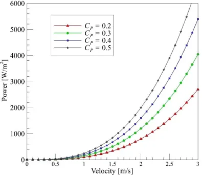
These turbines work on the same principle, where kinetic energy of the stream is utilized to rotate an electromechanical energy converter that generates electricity. The governing equation in such energy conversion is:

= 1₂ (1)

where P is the mechanical power extracted by the turbine [W], ρ is the density of the fluid (999.2 kg/m3 for water at 15 °C), A is the area of the rotor blades [m2], V is the fluid velocity [m/s] and CP is the power coefficient, a measure of the fluid-dynamic efficiency

of the turbine. The power coefficient CP tells how efficiently a turbine converts the

energy in the water to electricity and it depends on the electric system, mechanical system and blade hydrodynamic efficiency. This last one, the blade hydrodynamic efficiency, is the most important in the power output of the turbine because usually electrical and mechanical systems are well optimized already. For homemade turbines, this power coefficient stands between 10-15%, where 15% stands for a good homemade turbine. For commercialized turbines, these values of CP are somewhere between 30-40%.

Recently, a company by the name of “Smart Hydro Power” [4] started commercializing turbines with CP near 45% which is a big achievement in the in-stream turbines. Figure 2

(3)

Figure 2. Power output vs. velocity for different coefficients of power

To maximize the power output of the turbine, most of the time the channel width is reduced, so the velocities at the turbine entrance are of a higher order. But by narrowing the channel, environmental problems may surge because the characteristics of the channel are changing. The suggestion is to use the existing structures that narrow the channel by themselves to amplify the velocity. That’s the main focus of this study, to verify if some structures, in this case bank protection structures by the name of spur-dikes, change the velocity profiles in a way that can be used by hydro power generation devices and to achieve that, numerical simulations were conducted, using Computational Fluid Dynamics (CFD) software Ansys Fluent, where three cases with simple spur-dikes with different orientations in the channel were tested and compared with other case without spur-dikes so a conclusion can be reached if the behaviour of the water flow is similar to channel narrowing.

The introduction of spur-dikes into the river have the objective of:

• Make changes to the water flow so the river banks are protected by the erosion caused by it [5];

• Protect other structures like bridge piers [6, 7]; • Improve river navigability;

• Improve flood control [8];

• Ensure the water supply, for personal use and for irrigation, by stabilizing the flow velocity and the water level.

According to Zhang and Nakagawa [9], spur-dikes can be classified according to: • Permeability, them being permeable or impermeable;

• Angle, normal to the main stream, pointing downstream or upstream;

• Shape, taking different kinds of shapes, like “L” shape, “T” shape, rounded-head shape and so on.

As far as previous studies conducted by other authors and considering cases without spur-dikes first, some tested a simple channel with one simple bend [10, 11]. Other authors like Zhang and Shen [12] tested a model with a meandering channel similar to this study, but also without spur-dikes. In studies with simple, rectangular spur-dikes, some authors tested the local scour around it [13, 14]. Yazdi et al. [15] tested the velocity field around a single spur-dike. Li et al. [16] tested both velocity field changes and scour around spur-dike. There were authors who tested different shapes of spur-dikes such as

(4)

the L-Shaped spur-dike [17, 18]. Others tested the T-shape [19-21]. In what concerns simulations with hydropower devices, Sarma et al. [22] studied the possibility of the adaptation of Savonius wind turbines to the water environment, reaching good results even in relatively low velocity streams as well as low water height.

NUMERICAL MODELLING

Fluent CFD code was used for 3D numerical modelling. Numerical modelling involves the solution of the Navier-Stokes equations, which are based on the assumptions of conservation of mass and momentum within a moving fluid. When the principle of the conservation of mass is applied to a fluid particle in the flow, it can be expressed by the eq. (2):

= 0 (2)

The momentum equation can be described as shown in eq. (3):

= (3)

The term is known as the Reynolds Stresses and it needs modelling, using turbulence models so this equation system has a solution. To do so, the k-ω standard turbulence model is used. The turbulent kinetic energy (k) and the specific dissipation rate (ω) can be calculated using the transport equations shown as (4) and (5) [23]:

= ! " #! $! %! (4)

& & = ' &" #' $' %' (5) In these equations, Gk is the generation of turbulent kinetic energy due to the mean

velocity gradients, Gω represents the generation of ω, Γk and Γω represent the effective

diffusivity of k and ω, respectively. Yk and Yω represent the dissipation of k and ω due to

turbulence and Sk and Sω are user-defined source terms. The constants associated with the

calculation of each of the terms presented above are stated in Table 1.

Table 1. The k-ω standard turbulence model constants

()∗ () (+ ,)∗ , -. -! -' /∗ 01+ 2! 2'

1 0.52 1/9 0.09 0.072 8.0 6.0 2.95 1.5 0.25 2.0 2.0 VALIDATION

Before employing the numerical model to study the flow pattern around the spur-dike, it was necessary to ensure the accuracy of the numerical model. To do so, after the numerical model was completed, the results were compared with results of a study performed in a physical model by Vicario [24].

The experimental tests were carried out in a physical model located in Fluvial Hydraulic Laboratory from University of Beira Interior, which is a meandering channel with six sine-generated curves characterized by sinuosity of 1.2 and a wavelength equal

(5)

to 3.52 m. The maximum width of the channel is 0.68 m which corresponds to a discharge height dbf ≈ 0.125 m. The channel bed material is composed of uniform quartz sand [density, ρs = 2,660 kg/m3 (according to the NP-83, 1,965), d50 = 0.86 mm,

σD = 1.36]. The Banks are rigid and the side slope varies in order to remain as close as

possible to natural conditions. At crossover sections they are at 45°, increasing to 90° in the middle section of bend two and five.

For better understanding of the channel, Figure 3 presents a picture of the experimental setup where the plan view of the flume can be seen, as well as a three-dimensional model of the curve in focus in this study, with three sections highlighted (entrance, exit and central sections).

Figure 3. Experimental setup (a) and three-dimensional model of the bend in analysis (b)

Vicario [24] focused the study on the central section of the second bend, analyzing the velocity profiles in that section, after the channel bed reached an equilibrium state. Bed topography was later converted into a cad model, that was meshed to be used in the numerical model, so the replication of the channel was as close as possible to the original channel. Since the experimental studies were focused on the second bend of the channel, all the numerical models were focused on that bend as well.

Numerical model

In the mesh generation, an unstructured mesh type was adopted due to its adaptability to the problem geometry which was complex. A spacing between points in the isodepth lines was defined and blocks of meshes were assembled that once put together resulted in the final mesh block. Different spacing of points in the isolines were tested and refined until results were accurate enough, without expending an exorbitant amount of computational resources. The final mesh had a total of a little over 1 million points.

The boundary conditions were the following: • Entry section:

o Velocity inlet (U), with its characteristics described in Table 2 where values of mean velocity;

o Turbulent intensity (I); o Hydraulic diameter (D_H); o Water depth (Z);

o Reynolds Number (Re), are presented; • Bed and walls:

(6)

• Exit:

o Outflow; • Free surface:

o Wall with zero roughness.

Table 2. Flow characteristics at the inlet section

U [m/s] I [%] DH [m] Z [m] Re

0.36 3.4 0.345 0.12 ≈_31,000

To estimate the effect of wall on the flow, empirical wall functions known as standard wall functions [25] were used. The k-ω turbulence model was used with standard-wall functions. This model has advantages when there is strong recirculation flow such as in the case of spur-dikes.

To complete the description of the CFD modelling, the standard pressure discretization scheme was used, showing good convergence for the model, and first order upwind was used for the momentum, turbulent kinetic energy and specific dissipation rate discretization. As for Pressure-velocity coupling, the SIMPLE segregated algorithm was used. Convergence was reached when the normalized residual of each variable was on the order of 1 × 104 and it took the final mesh, which was composed of 1,085,307 nodes, between 28-30 hours to run. Computations were conducted using an Intel Core i7-4700MQ at 2.400 GHz processor and 8GB DDR3 of RAM memory.

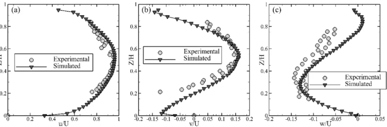
The results obtained are not a perfect match, because the model is based in the Reynolds-Averaged Navier Stokes equations, so there are some errors associated with the models. Also, the conversion of the bed topography to a cad model has some errors associated with it, and so do the experimental measurements. Ultimately, though not being a perfect match, it can be said that the results are very close and the differences can only be observed when the velocity scale is very small, like the ones in the transverse velocity and vertical velocity. Figure 4 shows the comparison between the simulated channel and the experimental one, as stated above.

Figure 4. Velocity profiles: longitudinal velocity (a); transverse velocity (b); vertical velocity (c)

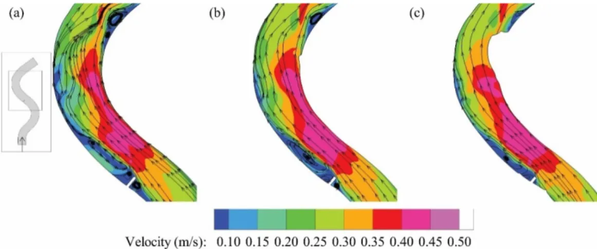
Plan view velocity profiles. From the study used to verify the numerical model, velocity profiles in a plan view were taken. These profiles were taken at three different depth levels, them being surface level, 3 cm deep and 6 cm deep. All of them are shown in Figure 5. Looking at Figure 5 it is clear that the velocity is of higher order in the inside of the bend. It is also visible that the highest velocity in each point is not at the surface but at about half of the water height, as the profile at 3 cm deep has higher velocity profiles than the surface one. This is also represented in Figure 4 where the highest longitudinal velocity is somewhere between 50% and 60% of the total height of water.

(7)

Figure 5. Plan view velocity profiles: surface level (a); 3 cm deep (b); 6 cm deep (c)

Cross-section profile. With this numerical simulation, it was possible to obtain the velocity field in a cross-section, in the middle of the second bend. This velocity field, when in cross-section, is also called secondary flow and it is one of the reasons erosion happens, apart from the shear stresses on the bed, because of the velocity field that goes straight into the bed on the outside of the bend, as it can be seen in the Figure 6.

Figure 6. Secondary flow in the central section of the second bend

The main reason this secondary flow is different from the one studied by Blanckaert [26] is that in this case we have a meandering channel. In that way, the double tubular secondary flow that is seen in his study does not appear, because he studied only one bend and not a meandering channel. So, in this case the bend before the one in analysis, the first bend in this channel, has influence on the secondary flow.

Figure 6 is intended to be a reference to other simulations, with spur-dikes, so it is possible to compare the effects of the secondary currents with and without the different kind of spur-dikes tested in this study.

SPUR-DIKES SIMULATIONS

Three cases with spur-dikes were modelled, with the spur-dikes inserted in the entry section of the second bend. All of them had a length with a ratio of 1/4 with the averaged width of the section, a width of 1/7 of the length and its inclination angle with upstream varied thus: Case 1 ‒ 90°, Case 2 ‒ 45° and Case 3 ‒ 135°. For all these cases, same mesh generation methods were used causing minor variations in the number of cells of each mesh, mainly because of the different shapes of spur-dikes.

Standard spur-dike (90º)

For the first case, a standard spur-dike was inserted into the flume, in the beginning of the second bend by the external zone. This specific kind of spur-dike is the simplest one,

(8)

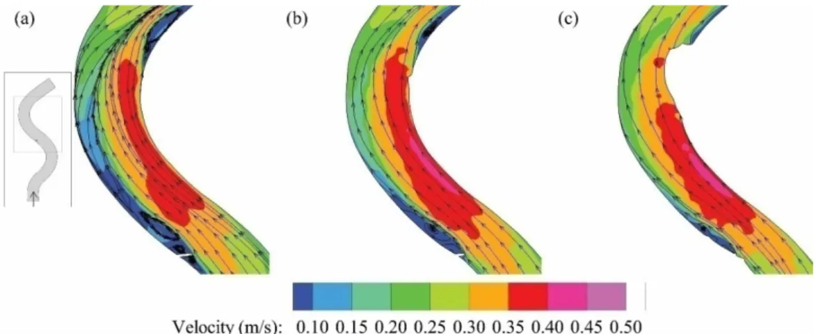
known usually by the name of deflecting spur-dike. The changes to the flow are obvious when this case is compared with the case without any spur-dikes. Comparing Figure 5 and Figure 7, it can be seen that the flow is deflected to the interior of the bend, increasing the flow velocity in that zone by about 25%.

Figure 7. Plan view velocity profiles: surface level; (a) 3 cm deep (b); 6 cm deep (c)

The return flow zone is also visible immediately after the spur-dike, where the velocity is nearly null and where vortexes of different dimensions appear. Analysing the different layers of the velocity magnitude, the maximum value for the velocity is not on top, following the same pattern of the case without the spur-dikes in it.

Cross section profile. With the spur-dike insertion into the flow field, the cross-section velocity profile at the middle of the second bend was, as expected, changed. The small vortex in the top of the exterior zone, got bigger and other vortexes appeared in the bottom, near the bed. The velocities increased about 50% as it is shown in Figure 8.

It is not expected that this change to the secondary flow caused an increase in erosion in the external part of the cross-section, because of the longitudinal velocity decrease in that area, causing its magnitude to be lower. That decrease causes the shear stress to decrease as well, so the erosion will decrease in this area.

Upstream angled spur-dike (45º)

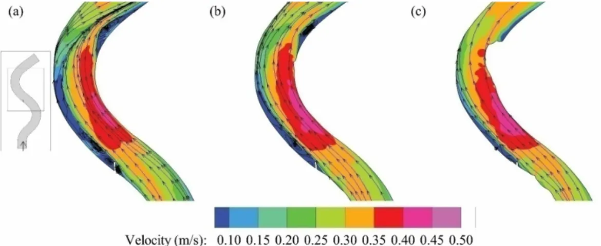
In the second simulation, a rectangular spur-dike pointing upstream was inserted into the flow. According to Zhang and Nakagawa [9], this type of spur-dikes is characterized by redirecting the flow away from the spur-dike. Analysing the velocity field shown in Figure 9 and comparing it to the standard spur-dike case, the velocity on the inside of the bend is lower than in the standard spur-dike case making it not as good as a velocity

(9)

amplifier for power production devices. Therefore, this case is not as aggressive to the bed of the channel as the previous case. As what concerns the outside region, this case offers a bigger zone of protection, where the velocities are lower, reaching almost the halfway of the bend. Under these circumstances, this spur-dike’s angle offers a better protection than the case one, although the increase of velocity in the inside of the bend is not as high as in the previous case, so for the purpose of power production this case has a worse behaviour than the previous one.

Cross section profile. Figure 10 represents the addition of the 45-degree upstream angled spur-dike. It caused the vortex in the top exterior to grow even bigger than in the standard spur-dike case, but in this case, the vortex near the bed was not formed, which came closer to the case where no spur-dike was inserted into the channel. As what concerns the secondary velocity intensity, it also increases but as much, being around 30% more than the case with no spur-dikes.

Downstream angled spur-dike (135º)

After testing the cases relative to a standard spur-dike and an upstream oriented one, this case concerns the downstream angled spur-dike. According to Zhang and Nakagawa [9], this spur-dike redirects the flow alongside the angle of it, making the flow deflection a lot smoother. Before any kind of analysis was done, it was expected that this case was going to offer worse results than the standard spur-dike, because of the smooth transition of the flow field to the centre of the curve. So, tests were made and the results are shown in Figure 11.

The results show that this case is not as aggressive to the bend as the standard spur-dike as it was expected and the velocity in the inside was not of as high order. Comparing it with the second case, this one increases the velocity a bit more than the case

(10)

2, making this narrowing of the channel a bit better for installing power production devices despite not being better than the standard spur-dike. As far as the outside region goes, the results are similar to the Case 2, presenting values for the velocity of the same order as well as similar extension of the protected area of the margin.

Cross section profile. In this case, of which results are presented in Figure 12 the behaviour of the secondary flow field was very close to the case of the upstream angled spur-dike. Both the streamlines and the velocity intensity were pretty much the same in the upstream angled case and the downstream angled spur-dikes. This might happen because both spur-dikes divert the fluid flow to the interior of the bend, making its behaviour really close.

ANALYSIS OF POWER PRODUCTION

After analysing the results on all three spur-dike cases, it can be stated that in all the cases, while successfully protecting the outside bank of the river channel, the spur-dikes also increased the velocity in the inside of the bend, making the initial assumption of the spur-dike in the channel behaving like a narrowing of the channel in that area, despite the spur-dike being thin. The velocity increases up to 22% in the case of the spur-dike that makes a 90-degree angle with the riverbank. While both downstream and upstream angled spur-dikes present lower increase of velocity, they still show a 12-17% increase which may not seem to be a lot if the analysis is made in this small-scale model used for testing, but looking into a real river where the velocities are usually more than 1.5 m/s, this percentage is much more influential. The scale model used was constructed in a way that it expresses the reality of a natural river, so all the parameters were carefully taken into account when constructing the channel so it was as real as possible. So, when an increment of 22% of the velocity happens in the channel even at a reduced velocity that it

(11)

runs, we can say that this increment will be of the same order in a real river with a much higher velocity.

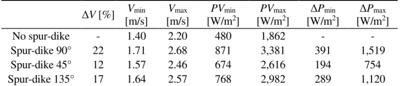
Table 3 shows the power output, calculated by using eq. (1), for the average interval of velocities of a river, 1.4-2.2 m/s, with a turbine CP of 0.35 and a blade area of 1 m2, for

cases with and without the spur-dikes, where the percentage of velocity increase due to the structures analysed in this study are considered.

The chosen coefficient of power for the calculations was 0.35, a value for a very well optimized turbine. Although certain companies reached CP’s of nearly 0.45, it is still not

so common value for most turbines and it is very hard to achieve such efficiencies. So a much more conservative value was chosen for the efficiency. The 1 m2 _{of blade area was} used just to make the calculations so that comparisons with other turbine areas could be made a lot easier.

Table 3. Summary of power output for each case with velocities of a common river

Δ_V_[%] Vmin [m/s] Vmax [m/s] PVmin [W/m2] PVmax [W/m2] Δ_P_min [W/m2] Δ_P_max [W/m2] No spur-dike - 1.40 2.20 480 1,862 - - Spur-dike 90° 22 1.71 2.68 871 3,381 391 1,519 Spur-dike 45° 12 1.57 2.46 674 2,616 194 754 Spur-dike 135° 17 1.64 2.57 768 2,982 289 1,120

As it can be observed, the effect of spur-dikes in a normal in-stream turbine, for a velocity increase ΔV of 12-22%, its power output can increase from 200 W up to 1,500 W which is a major achievement if the maximization of power output, the main objective of the research. In the case of the 90° spur-dike, the maximum potential increment is almost doubled, which means that the same turbine is putting out almost double the power. Achieving this by carefully placing the power production devices in some specific zones of a channel may be a major money saver for those who only want a certain amount of power produced, to support an irrigation pump for example. It saves money to the investor, by generating what in normal situations should take almost double the turbines of that type to generate that amount of power.

CONCLUSION

Spur-dikes behave as expected, granting a good zone of protection on the outside of the bend, where the velocities are lower and went up on the inside of the bend. This created a zone where power production devices such as turbines can be inserted, generating up to 85% more power than in a normal situation without spur-dikes in the river.

ACKNOWLEDGMENT

For the financial support, the authors wish to thank the Portuguese Foundation for Science and Technology (FCT) within the Grant ERANETMED/0004/2014, through the ERANETMED initiative of Member States, Associated Countries and Mediterranean Partner Countries (Project ID eranetmed_nexus-14-044) and within the UID/ECI/04082/2013.

NOMENCLATURE

A area [m2]

(12)

D50 bed median grain size [mm]

dbf bankfull height of channel [m]

H maximum channel height [m]

k turbulent kinetic energy [m2_/s2_]

P power [W]

p pressure [N/m2]

t time [s]

u instantaneous velocity [m/s]

u’ fluctuation of velocity [m/s]

V volume [m3_]

x particle position [m]

Z channel height at cross section [m]

Greek letters

ρ density [kg/m3]

ω specific dissipation rate [1/s]

μ dynamic viscosity [N s/m2]

REFERENCES

1. Greenpeace, Decentralising Power: An Energy Revolution for the 21st Century, London, UK, 2005.

2. Aurora Power & Design, 1000W Low-Head Kaplan Hydro Turbine, 2017, https: //www.aurorapower.net/products/categoryid/4/list/1/level/a/productid/234.aspx, [Accessed: 01-June-2017]

3. Khan, M. J., Bhuyan, G., Iqbal, M. T. and Quaicoe, J. E., Hydrokinetic Energy Conversion Systems and assessment of Horizontal and Vertical Axis Turbines for River and Tidal Applications: A Technology Status Review, Applied Energy, Vol. 86, No. 10, pp 1823-1835, 2009, https://doi.org/10.1016/j.apenergy.2009.02.017

4. Smart Hydro Power, Smart Hydro Power, 2017, http://www.smart-hydro.de/, [Accessed: 01-March-2017]

5. Kuhnle, R., Jia, Y. and Alonso, C., Measured and simulated Flow near Spur Dikes,

Journal of Hydraulic Engineering, Vol. 134, No. 7, pp 916-924, 2008,

https://doi.org/10.1061/(ASCE)0733-9429(2008)134:7(916)

6. Karaki, S., Hydraulic Model study of Spur Dikes for Highway Bridge openings, 1959.

7. Herbich, J. B., Spur Dikes prevent Scour at Bridge abutment, 1966.

8. JICA-DPWH, Technical Standards and Guidelines for design of Flood Control Structures, 2010.

9. Zhang, H. and Nakagawa, H., Measured and simulated Flow near Spur Dikes,

Annuals of Disas. Prev. Res. Inst., Vol. 51B, pp 633-652, 2008.

10. Abhari, M. N., Ghodsian, M., Vaghefi, M. and Panahpur, N., Experimental and Numerical Simulation of Flow in a 90 Degree Bend, Flow Measurement and

Instrumentation, Vol. 21, pp 292-298, 2010,

https://doi.org/10.1016/j.flowmeasinst.2010.03.002

11. Gholami, A., Akhtari, A. A., Minatour, Y., Bonakdari, H. and Javadi, A. A., Experimental and Numerical Study on Velocity Fields and Water Surface Profile in a Strongly-curved 90° open Channel Bend, Engineering Applications of Computational

Fluid Mechanics, Vol. 8, No. 3, pp 447-461, 2014,

https://doi.org/10.1080/19942060.2014.11015528

12. Zhang, M. and Shen, Y., Three-dimensional Simulation of meandering River based on 3-D RNG k-ε Turbulence Model, Journal of Hydrodynamics, Vol. 20, No. 4, pp 448-455, 2008, https://doi.org/10.1016/S1001-6058(08)60079-7

(13)

13. Fazli, M., Ghodsian, M. and Neyshabouri, S., Scour and Flow Field around a Spur Dike in a 90 Bend, International Journal of Sediment Research, Vol. 23, No. 1, pp 56-68, 2008, https://doi.org/10.1016/S1001-6279(08)60005-0

14. Rashedipoor, A., Masjedi, A. and Shojaenjad, R., Investigation on Scour Hole around Spur Dike in a 80 Degree Flume Bend, World Applied Sciences Journal, Vol. 19, pp 924-928, 2012, https://doi.org/10.5829/idosi.wasj.2012.19.07.1711

15. Yazdi, J., Sarkardeh, H., Azamathulla, H. M. and Ghani, A. A., 3D Simulation of Flow around a single Spur Dike with Free-surface Flow, International Journal of

River Basin Management, Vol. 8, No. 1, pp 55-62, 2010,

https://doi.org/10.1080/15715121003715107

16. Li, G., Lang, L. and Ning, J., 3D Numerical simulation of flow and Local Scour around a Spur, IAHR World Congr., Chengdu, China, 2013.

17. Matinfard, A., Heidarnejad, M. and Ahadian, J., Effect of changes in the Hydraulic Conditions on the Velocity distribution around a L-shaped Spur Dike at the River Bend using Flow-3D Model, pp 1862-1868, 2013.

18. Suhai, K., Study on current Field around the Spur-dike with 3-D Numerical simulation, E-Proceedings of 36th IAHR World Congr., The Hague, Netherlands, pp 1-6, 2015.

19. Masjedi, A., Bejestan, M. S. and Rahnavard, P., Reduction of Local Scour at Single T-shape Spur Dike with Wing Shape in a 180 Degree Flume Bend, World Applied

Sciences Journal, Vol. 8, No. 9, pp 1122-1128, 2010.

20. Vaghefi, M., Ahmadi, A., Faraji, B., Javan, M. and Eghbalzadeh, A., Numerical Study of Flow Patterns around T shape Spur Dike and support Structure, Journal of

River Engineering, Vol. 2, No. 5, 2014.

21. Daneshfaraz, R., Ghaderi, A. and Ghahremanzadeh, A., An analysis of flowing pattern around T-shaped Spur Dike at 90° Arc, based on Fluent and Flow-3D Models,

International Bulletin of Water Resources & Development, Vol. 3, No. 3, pp 1-9,

2015.

22. Sarma, N. K., Biswas, A. and Misra, R. D., Experimental and Computational evaluation of Savonius Hydrokinetic Turbine for Low Velocity condition with comparison to Savonius Wind Turbine at the same Input Power, Energy Conversion

and Management, Vol. 83, pp 88-98, 2014,

https://doi.org/10.1016/j.enconman.2014.03.070

23. Wilcox, D. C., Turbulence Modeling for CFD, DCW Industries, Incorporated, 1994. 24. Vicario, S. A., Characterization of Flow in a Meander Channel, Final Degree Project

for obtaining the Degree in Civil Engineering, Mención Hidrologia, University of Salamanca, Salamanca, Spain, 2016.

25. Launder, B. E. and Spalding, D. B., The Numerical computation of Turbulent Flows,

Journal of Computer Methods in Applied Mechanics and Engineering, Vol. 3, No. 2,

pp 269-289, 1974, https://doi.org/10.1016/0045-7825(74)90029-2

26. Blanckaert, K. and De Vriend, H. J., Secondary Flow in Sharp Open-channel bends,

Journal of Fluid Mechanics, Vol. 498, pp 353-380, 2004,

https://doi.org/10.1017/S0022112003006979

Paper submitted: 04.10.2017 Paper revised: 28.11.2017 Paper accepted: 28.11.2017