CARBON FOOTPRINT IN DEHESA AGROFORESTRY
SYSTEMS
Escribano M1, Moreno G2, Eldesouky A1, Horrillo A1, Gaspar P1, Mesías FJ1*
(1) Research Institute of Agricultural Resources (INURA). University of Extremadura. Avda. Adolfo Suarez. s/n 06007 Badajoz, Spain (2) INDEHESA - Institute for Silvopastoralism Research. University of Extremadura. Plasencia 10600,
Spain
*Corresponding author: [email protected]
Abstract
Dehesa agroforestry systems (rangelands located in Southwest Spain) are characterised by their semi-arid and often marginal conditions. In this sense, the study of the role of carbon footprint in extensive systems is of great interest by analysing, within a case study framework, the two production systems available in dehesa farms and providing the methodological adjustments required to generate results that are comparable with other livestock systems and species. Results have revealed that sheep meat farms are those with the lowest carbon footprint levels (14.06 kg CO2eq/kg live weight), followed by meat production farms selling calves at weaning period. Enteric fermentation accounts for 64.10% to 48.99% of the total emissions, and it is linked to the extensification of these systems and to the grazing diet of the Undoubtedly, feeding is the input that amounts for the highest percentage of off-farm emissions, as it can reach up to 24.90%.
Keywords: carbon footprint, life cycle assessment, extensive production, greenhouse gases
Introduction
Extensive grazing systems located in the Southwest of Spain are characterized by their semi-arid and often marginal conditions with poor soils and scarce and irregular rainfall. These features are behind the low supply of pastures available for livestock use so that proper management is based on the use of reduced stocking rates which imply a minimal animal pressure on the territory. These systems share some of the characteristics defined for extensive animal production systems, such as the limited number of animals per hectare, low productivity per animal and hectare and feeding mainly based on free-range grazing and the use of agricultural by-products.
In this context, the environmental impacts of the agricultural or livestock production depend to a great extent on the production systems, which can be influenced by techniques, harvesting period and other technical issues. This primary phase is seen as the main contributor to the environmental impacts of food, related to biodiversity loss GHG emissions and reduction of soil fertility, among others.
Among livestock food products, meat has the greatest environmental impact. This is due to the inefficiency of animals in converting feed to meat, as 75 90% of the energy consumed is needed for body maintenance or lost in manure and by-products such as skin and bones. There are many processes contributing to major GHG emissions during meat production are: (1) production of feed, (2) enteric fermentation from feed digestion by animals (mainly ruminants), (3) manure handling and (4) energy use in animal houses.
Therefore, analysis of the carbon footprint (CF) in livestock production identifies the production procedures or techniques in which emissions may be reduced using improved efficiencies, estimates the amount and breakdown of GHG emissions and provides a mechanism to track efforts in improving efficiencies and reducing emissions.
Strangely enough, at least when it comes to environmental issues, intensifying animal production is generally advocated to mitigate certain environmental impacts, such as emission of greenhouse gases associated with production of animal-source food (Steinfeld and Gerber 2010). In this regard, the intensification of animal production in feedlots or with changes in their diet allows the early slaughter and has been reported as a strategy adopted in several countries to reduce GHG emissions in the production of beef (Ruviaro et al. 2016).
With that in mind, many consumers are still unfamiliar with carbon footprint information. making it difficult for them to evaluate and compare the different products which are offered. However, meat companies are interested in finding how different product characteristics can influence consumer choices and whether there is a possibility for a price premium if products are differentiated using the carbon footprint attribute. This topic is especially relevant in extensive systems, where environmental values associated to livestock production can be overshadowed by the comparatively higher emissions of these production systems.
The methodology selected in this research is the Life Cycle Assessment (LCA), a quantitative and environmental assessment of a product over its entire life cycle, including raw material acquisition, production, transportation, use and disposal (Khasreen et al. 2009). LCA attempts to quantify the materials and energy consumed, and chemicals emitted to the environment during resource extraction, manufacturing, distribution, use, and end-of-life stages of a product/service.
In this sense, it is of great interest to study the role of CF in extensive systems, analysing, within a case study framework, the different production systems present in dehesa agroforestry systems and providing the methodological adjustments required to generate results comparable with other livestock systems and species.
Materials and methods
Among the different methodologies available to estimate the GHG emissions, Life cycle assessment (LCA) is an internationally accepted, standardized methodology for quantifying the environmental impact of a product, and it has been therefore selected for this research.
CF calculation has been made in accordance with British standard PAS 2050 and the IPCC the methodology cited by the Spanish Ministry of Agriculture has been followed regarding the characteristics of livestock in the analyzed areas and manure management (MAPAMA 2012). The process followed in this has consisted on the study of carbon footprint within the context of
Data collection
This study is based on the analysis of two different case studies. Data were obtained through the monitoring of two farms through field visits and interviews with farmers carried out between January and May of 2017. The following case studies were analysed, as they were considered to be the most representative of the extensive systems in the Mediterranean agroforestry systems: Extensive meat sheep farming and Extensive beef/veal cattle farming
Functional unit
In this paper, the functional unit (FU) is the reference unit with which all the produced emissions of the system will be associated. The FU varies according to the analyzed case and taking as a
Estimation of GHG emissions and calculation of CF in farms
Global Warming Potentials proposed by the IPCC have been used to convert the raw data of methane (CH4) or nitrous oxide sources (N2O) emissions. Each gas has a specific value, 1 for CO2, 25 for CH4 and 298 for N2O. In this way, data from raw emissions of CH4 and N2O gases are multiplied by 25 and 298, respectively, to transform this data to kg CO2 equivalent.
In order to estimate the emissions, the emission factors of the gases produced by the system have been used, in addition to the inputs shown in Table 1.
Table1: Emission factors used to quantify GHG emissions of the analysed farms in the baseline scenario.
Emission and source Type GHC of EF Into de systems
Enteric fermentation CH4 8.64 kg CH4/Sheep head yeara
57 kg CH4/Cow head year
Manure management
Manure management CH4 CH4 (0.19 e 0.37 in sheep)b kg CH4/head
year
2.70 in Bovine kg CH4/head year
Manure management direct N2O N2O 0.005 kg N2O eN/kg N Solid storage
system
Manure management indirect N2O N2O 0.01 kg N2O eN /volatilized
Soil management
N from organic fertilizers (compost. manure) N2O 0.01 kg N2O eN (kg N input)-1
N from urine and dung inputs to grazed soils in
Sheep N2O 0.01 kg N2O eN (kg N input)
-1
N from urine and dung inputs to grazed soils in Cow N2O 0.02 kg N2O eN (kg N input)-1
Indirect emissions Management Soils N2O 0.01 kg N2O eN (kg % N
volatilised/leaching)-1 Out of the systems
Concentrates Meat Sheep CO2 0.512 kg CO2eq/kg
Concentrates Meat Cow CO2 0.512 kg CO2eq/kg
Forages CO2 0.100 kg CO2eq/kg
Electricity CO2 0.308 kg CO2eq/kWh
Diesel CO2 2.664 kg CO2eq/litre - combustion
0.320 kg CO2eq/litre - upstream
Most of the emission factors have been taken from IPCC Guidelines (2006). Vol 4. Chapter 10 and 11. a Emission factor adapted to the area. MAPAMA (2012)
b With average temperature
Results
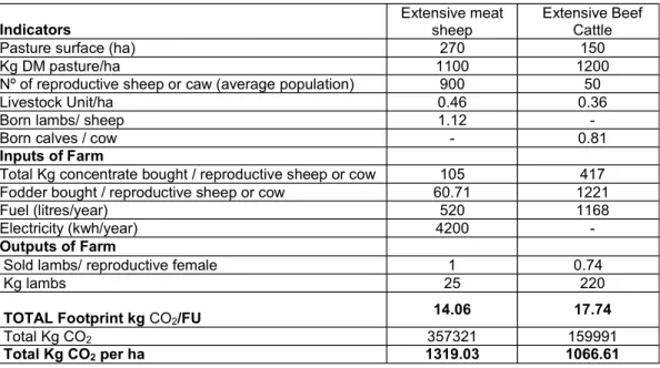
The studied farms correspond to the dehesa extensive systems that are devoted to the production of meat sheep and calves at weaning age. Table 2 shows the technical characteristics of these farms, together with estimated footprint, wich is 14.06 kg CO2 / kg FU in the case of sheep and of 17.74 kg CO2 / kg FU in beef.
Table 2: Technical indicators & Carbon footprint of the studied farms.
Indicators Extensive meat sheep Extensive Beef Cattle
Pasture surface (ha) 270 150
Kg DM pasture/ha 1100 1200
Nº of reproductive sheep or caw (average population) 900 50
Livestock Unit/ha 0.46 0.36
Born lambs/ sheep 1.12 -
Born calves / cow - 0.81
Inputs of Farm
Total Kg concentrate bought / reproductive sheep or cow 105 417 Fodder bought / reproductive sheep or cow 60.71 1221
Fuel (litres/year) 520 1168
Electricity (kwh/year) 4200 -
Outputs of Farm
Sold lambs/ reproductive female 1 0.74
Kg lambs 25 220
TOTAL Footprint kg CO2/FU 14.06 17.74
Total Kg CO2 357321 159991
Total Kg CO2 per ha 1319.03 1066.61
However when considering emissions in relation to the territory it can be seen that the emission levels are lower in the case of cattle with 1066.67 kg CO2 / ha compared to 1319.03 kg CO2/ ha of sheep. In this sense, the current system of linking the produced emissions to the product units is questioned, at least in dehesa agroforestry systems, characterized by extensification and low levels of production.
In Figure 1 we analyze the percentage contribution of the different greenhouse gases in the different processes, whether they are produced on the farm itself or due to inputs.
Discussion
Undoubtedly, feed is the highest input of the farm's emissions percentage, reaching up to 24.90% of the total in cattle farms and compared to 21.20% in sheep meat.
Enteric fermentation and feeding are the factors that produce the greatest range of emissions and their distribution will be largely conditioned on the operating based systems or not grazing systems. We can also observe its relation with the final carbon footprint, since the farms that have important feed inputs tend to have a smaller footprint because the number of product units increases.
In extensive systems, mitigation strategies should be aimed at increasing the digestibility of pastures that generally reduce GHG emissions from enteric fermentation and stored manure. In parallel, it should be noted that these systems cannot compete in product units with more intensive ones and therefore the carbon footprint in dehesa agroforestry systems should be referred to the territory. The compensation of their emissions due to carbon sequestration by carbon sinks also needs to be highlighted.
Conclusions
LCA is a useful tool for measuring the potential environmental performance of livestock production. LCA may be combined with other methods to assess economic sustainability of animal production in order to reveal on-farm efficiencies. It also could help reduce both environmental and monetary costs associated with animal rearing.
However, extensive farms usually have a territorial component (hectares of agricultural land, CO2 emissions, due to carbon sequestration. Nevertheless, it is not common to take into account carbon sequestration in LCA studies, which creates a disadvantage for extensive systems, and can send confusing messages to the consumers and endanger the persistence of these valuable and complex systems.
References
IPCC (2006) IPCC guidelines for national greenhouse Gas inventories. In: Inter-governmental Panel of Climate Change (IPCC). National Greenhouse Gas Inventories Programme.
MAPAMA (2012) Inventarios Nacionales de Emisiones a la Atmósfera 1990-2012. Volumen 2: Análisis por Actividades SNAP. Capítulo 10: Agricultura.
Khasreen MM, Banfill PF, Menzies GF (2009) Life-cycle assessment and the environmental impact of buildings: a review. Sustainability 1: 674-701.
Ruviaro CF, da Costa JS, Florindo TJ, Rodrigues W, de Medeiros GIB, Vasconcelos PS (2016) Economic and environmental feasibility of beef production in different feed management systems in the Pampa biome. southern Brazil. Ecol Indic 60: 930-939.
Steinfeld H, Gerber P (2010) Livestock production and the global environment: consume less or produce better? PNAS 107: 18237 18238.