Pedro Manuel Duarte Gonçalves Amaro
M.Sc. in Physics Engineering
Study of Forbidden Transitions in
Atomic Systems
A Thesis submitted for the co-tutelle degree of Doctor in Physics at Universidade Nova de Lisboa and Université Pierre et Marie Curie
Supervisor: José Paulo dos Santos, Professor com
Agregação, Faculdade de Ciência e
Tecnologia da Universidade Nova de
Lisboa
Supervisor: Paul Indelicato, Directoire de le recherche,
Université Pierre et Marie Curie, École
Normale Supérieure, Laboratoire Kastler
Brossel
Examination committee
Chair: Prof. Maria Adelaide de Almeida Pedro de Jesus Examiner: Prof. Michel René Jean Godefroid
Examiner: Prof. Joaquim Marques Ferreira dos Santos
Other Members: Prof. Alfred Maquet
Prof. José Paulo Moreira dos Santos
Prof. Fernando António de Freitas Costa Parente
T
h
ese de doctorat en cotutelle
`
Discipline : Physique
pr´esent´ee par
Pedro Manuel Duarte Gonc¸alves A
maro
´
ETUDE DES TRANSITIONS INTERDITES DANS
SYST `
EMES ATOMIQUES
pour obtenir le grade de Doctor de
Universit´e Pierre et Marie Curie
etUniversidade Nova de Lisboa
Dirig´ee par Jos´e Paulo dos Santos et Paul Indelicato
Soutenue le 20 december 2011 devant le jury compos´e de:
Maria Adelaide
de
J
esus
Universidade Nova de Lisboa
pr´esident
Michel Godefroid
Universit´e Libre de Bruxelles
examinateur
Joaquim dos Santos
Universidade de Coimbra
examinateur
Alfred Maquet
Universit´e Pierre et Marie Curie rapporteur
Study of Forbidden Transitions in
Atomic Systems
Pedro Manuel Duarte Gonc¸alves Amaro
FCT-UNL UPMC
Study of Forbidden Transitions in Atomic Systems.
Copyright c2011 Lisbon.
Pedro Manuel Duarte Gonc¸alves Amaro, FCT, UNL and UPMC. All rights reserved.
I start my acknowledgements by expressing my deepest gratitude to my supervisor, Prof. J. P. Santos, who introduced me to the world of science and physics. During the last years, his suggestions and guidance were crucial for bringing my work to a good port.
Next, I give my sincere gratitude to my co-supervisor, Dr. P. Indelicato for accepting and welcoming me in the LKB at Paris. His corrections and critics are highly acknowledged. During my stay in Paris I had many discussions that helped me overcome the various problems of the lab and improved my understanding of the involved physics. Therefore, I express my gratitude to Dr. Alexandre Gumberidze, Dr. Alexandre Vallette, Dr. Csilla, Dr. Eric, Dr. Martino, and Dr. Sophie. Additionally, I would like to thank Prof. Andrey and Dr. Filippo for welcoming me in Heidelberg and for the nice scientific discussions.
Pelo ambiente amig´avel na FCT, quero agradecer aos meus colegas, Diana, Diogo, Mauro, Dr. Rodrigo, Rui, Sandro e Vitor.
N˜ao me podia esquec¸er das pessoas mais queridas. Agradec¸o `a minha familia pela motivac¸˜ao e suporte. Aos meus sobrinhos, por toda a alegria e mimos que me d˜ao. A minha m˜ae merece um obrigado especial. Com todos os problemas que o destino lhe apresentou, sempre me deu o maior apoio, atenc¸˜ao e amor. Pelos momentos felizes que construimos juntos, agradec¸o-te, Susana. Sem a vossa atenc¸˜ao e carinho n˜ao era poss´ıvel concluir este trabalho.
The work reported in this Thesis was performed in collaboration with:
• Centro de F´ısica At´omica (CFA) group of Faculdade de Ciˆencias e Tecnologia
(FCT) of Universidade Nova de Lisboa (UNL).
• M´etrologie des Syst`emes Simples et tests Fondamentaux group of the Laboratoire
Kastler Brossel (LKB). LKB is a unit´e mixte de recherche n◦ 8552 of the ´Ecole
Normale Sup´erieure ENS, Centre National de la Recherche Scientifique (CNRS) and Universit´e Pierre et Marie Curie UPMC.
• APIX group in Heidelberg University.
Support for performing this Thesis was provided by:
• Acc¸˜oes Integradas Luso-Alem˜as (Contract noA-19/09)
• Fundac¸˜ao de Ciˆencias e Tecnologia (FCT), contract SFRH/BD/37404/2007. FCT
belongs to the Portuguese Ministry of Science, Technology and Superior Education (MCTES). Funds from Programa Operacional Potencial Humano (POPH/FSE) and
One active topic in Atomic Physics is the study of highly charged ions (HCI). These physical systems have a strong Coulomb field that provides a unique opportunity to in-vestigate and validate relativistic, Quantum ElectroDynamics (QED), and many-body effects. Moreover, fundamental test on symmetries and parity violation gives clues to the
physics beyond the Standard Model. Thus, nowadays, a primary goal of Atomic Physics is the existence of precise experimental data and accurate theoretical calculations for these systems.
In this thesis I focus on the investigation of forbidden radiative transitions in HCI. The main emphasis of this work is on atomic transitions, in which the selection rules forbids the emission of electric dipole photons. In this special type of radiative transition, the electron decays mainly through the emission of a single magnetic dipole photon, or two electric dipole photons. Both types of decay are investigated either experimentally or theoretically.
The two-photon decay is only theoretically investigated, using a full relativistic formal-ism, in HCI with one or two electrons. Several physical effects in the two photon decay,
such as resonances, the Dirac’s negative continuum or angular correlations are consid-ered. Related with the decay, two-photon excitation is also investigated. According to these evaluations, I stress the importance of relativistic and nondipolar effects.
More-over, a new approach based on the B-polynomials basis set is employed on two-photon transitions.
The second part of the work is devoted to the precise measurement of transitions in highly charged Ar with two to four electrons. For that matter, I describe the technical features of a double crystal spectrometer used to perform those measurements in HCI for the first time. This kind of spectrometer is able to perform absolute and precise measurements with an accuracy never achieved in these systems, which enables a comparison with re-cent QED calculations. I describe a Monte-Carlo code developed with the purpose of studying several systematic errors, as well as testing the various methods of retrieving physical quantities from raw data. Finally, I present the first absolute 2 ppm measure-ments on HCI with this spectrometer, paying special attention on the forbidden magnetic dipole transition in He-like Ar.
Keywords: Forbidden transitions, HCI, QED, Multi-photon processes, ECRIS, X-ray spectroscopy, Monte-Carlo simulation.
L’´etude des ions fortement charg´es connaˆıt un fort d´eveloppement en physique atomique. Ces syst`emes physiques permettent d’´etudier et valider la th´eorie de l’´electrodynamique quantique en champ fort, et les m´ethodes du probl`eme `a n-corps relativiste. Par ailleurs, r´ealiser des tests de physique fondamentale sur les sym´etries, comme par exemple la violation de la parit´e peut donner des indications sur une ´eventuelle physique au-del`a du Mod`ele Standard. Un des principaux objectifs de la physique atomique moderne est ainsi d’obtenir des donn´ees exp´erimentales pr´ecises et pour tester les calculs th´eoriques sur ces syst`emes.
Cette th`ese est consacr´ee `a l’´etude des transitions radiatives interdites dans les ions lourds multicharg´es. En particulier, j’ai ´etudi´e les transitions atomiques, dans lesquelles les r`egles de s´election interdisent les d´esexcitations de type dipolaire ´electrique. Dans ces transitions interdites, les ´etats excit´es m´etastables se d´esexcitent par transition dipolaire magn´etique, ou par des transitions `a deux photons de type ´electrique dipolaire. Les deux types de d´esexcitation ont ´et´e ´etudi´es exp´erimentalement et th´eoriquement dans les ann´ees r´ecentes.
Dans ce travail, j’ai r´ealis´e l’´etude th´eorique de la d´esexcitation `a deux photons pour des ions tr`es charg´es avec un ou deux ´electrons, en utilisant un formalisme relativiste. J’ai consid´er´e plusieurs effets physiques dans l’´etude de ces ph´enom`enes, tels que celui
des r´esonances, du continuum n´egatif de Dirac ou des corr´elations angulaires. J’ai aussi ´etudi´e l’effet inverse, l’excitation `a deux photons. Grˆace `a ces calculs j’ai pu mettre
en ´evidence l’importance des effets relativistes et des multipoles d’ordre sup´erieur. Par
ailleurs, j’ai d´evelopp´e une nouvelle approche num´erique fond´ee sur l’utilisation d’une nouvelle famille de fonction de base appel´ee B-polynmes pour le calcul de la transition `a deux photons.
La deuxi`eme partie de la th`ese est consacr´ee `a la mesure pr´ecise d’´energies de transi-tions radiatives dans des ions Ar tr`es charg´es, avec de deux `a quatre ´electrons. Dans cette partie, je d´ecris les caract´eristiques techniques d’un spectrom`etre `a deux cristaux plans, que nous avons utilis´e pour effectuer ces mesures, ce qui une premi`ere pour des
ions tr`es charg´es. Ce type de spectrom`etre permet d’effectuer des mesures absolues avec
une pr´ecision jamais atteinte dans ces syst`emes, ce qui permet une comparaison avec des calculs de QED les plus r´ecents. Je d´ecris le code de simulation du spectrom`etre, bas´e sur la m´ethode de Monte-Carlo, que j’ai d´evelopp´e dans le but d’´etudier plusieurs erreurs syst´ematiques, ainsi que pour tester les diff´erentes m´ethodes d’extraction de l’´energie et
terdite dipolaire magn´etique dans l’argon `a deux ´electrons.
The work performed in this Thesis was published in the following list, which contains also manuscripts for publication.
• P. Amaro, J. P. Santos, F. Parente, A. Surzhykov, and P. Indelicato. Resonance ef-fects on the two-photon emission from hydrogenic ions. Phys. Rev. A, 79(6):062504, 2009.
• A. Surzhykov, J. P. Santos, P. Amaro, and P. Indelicato.Negative-continuum effects on the two-photon decay rates of hydrogenlike ions. Phys. Rev. A, 80(5):052511, 2009.
• P. Amaro, A. Surzhykov, F. Parente, P. Indelicato, and J. P. Santos. Calculation of two-photon decay rates of hydrogen-like ions by using B-polynomials. J. Phys. A: Math. Theor., 44(24):245302, 2011.
• A. Surzhykov, P. Indelicato, J. P. Santos, P. Amaro, and S. Fritzsche. Two-photon absorption of few-electron heavy ions. Phys. Rev. A, 84(2):022511, 2011.
• P. Amaro, F. Fratini, S. Fritzsche, P. Indelicato, J. P. Santos and A. Surzhykov.
Parametrization of the angular and polarization in two-photon decays of
hydrogen-like ions. Manuscript for publication.
• P. Amaro, S. Schlesser, M. Guerra, E. O. Le Bigot, J. M. Isac, P. Travers, J. P.
Santos, C. I. Szabo, A. Gumberidze, and P. Indelicato, Absolute measurement of the “relativistic M1” transition energy in heliumlike argon. Submitted to Physical Review Letter.
• P. Amaro, C.I. Szabo, S. Schlesser, A. Gumberidze, E.O. Le Bigot, M. Guerra, J.
List of Contents
List of Figures xv
List of Tables xix
Nomenclature xxi
1 Forbidden Transitions 1
I Two-Photon Transitions 5
2 Introduction to Two-Photon Transitions 7
3 Theory of Two-photon Transition 11
3.1 One electron Dirac equation . . . 12
3.1.1 Free electron . . . 12
3.1.2 One electron in a nucleus potencial . . . 13
3.2 QED . . . 17
3.2.1 S Matrix in interaction representation . . . 18
3.2.2 Quantified field . . . 19
3.2.3 S Matrix for two-photon transition . . . 21
3.3 Two-photon emission . . . 23
3.3.1 Multipole expansion for the total decay rate . . . 24
3.4.1 Finite basis set approach to the Dirac equation . . . 31
3.4.2 Spurious states and boundary conditions . . . 33
3.4.3 B-splines . . . 34
3.4.4 B-polynomials . . . 35
3.4.4.1 Description of B-polynomials . . . 35
3.4.4.2 Energies obtained with B-polynomials basis set . . . 38
3.4.4.3 Analytical expression for the radial matrix elements . . . 39
3.5 Negative contribution to the two-photon emission . . . 39
3.6 Two-photon emission angular and polarization correlations . . . 41
3.7 Resonant transitions . . . 43
3.7.1 Line profile approach . . . 45
3.7.2 Two-loop self-energy . . . 46
3.7.3 Integration method for resonant intermediate states . . . 46
3.8 Two-photon excitation . . . 50
4 Results for Two-photon Transitions 53 4.1 Optimization of the numerical evaluation . . . 53
4.1.1 B-splines . . . 53
4.1.2 B-polynomials . . . 55
4.2 Negative continuum contribution in two-photon emission . . . 60
4.3 Angular correlations and polarization in two-photon emission . . . 67
4.4 Resonance states . . . 76
4.5 Two-photon excitation . . . 87
4.6 Preliminary results in He-like Ions . . . 91
5 Conclusion 95
II Measurement of Forbidden Transitions with a Double Crystal Spectrometer 99
6.1 Double Crystal Spectrometer . . . 102
6.2 Experimental setup . . . 106
6.2.1 ECRIS . . . 106
6.2.2 DCS . . . 106
6.2.3 Alignment . . . 109
7 Theory and Simulation of the Double Crystal Spectrometer 113 7.1 Dynamical theory of X-ray diffraction . . . 113
7.2 Theory of the DCS . . . 117
7.2.1 Study of the rocking curves . . . 121
7.2.1.1 Parallel rocking curve . . . 124
7.2.1.2 Antiparallel rocking curve . . . 125
7.3 Simulation of the DCS . . . 126
7.3.1 Path between the source and first crystal . . . 127
7.3.2 Generation of a random wavelength and a Bragg angle . . . 130
7.3.3 X-ray Reflection in first crystal . . . 132
7.3.4 Path from first crystal to detector . . . 133
7.4 Data analysis . . . 134
7.4.1 χ2fitting . . . 136
7.4.2 Voigt functions . . . 137
7.5 Study of systematic errors . . . 138
7.5.1 Vertical misalignment . . . 138
7.5.2 Crystal tilt . . . 139
7.5.3 Both vertical misalignment and crystal tilt . . . 140
7.5.4 Horizontal geometrical error . . . 145
7.5.5 Crystals bent . . . 146
7.5.6 Crystals miscut . . . 149
8 Experimental Results on Double Crystal Spectrometer 153
8.1 Study of Systematic Errors . . . 153
8.2 1s2s3S1→1s2 1S0in He-like Ar . . . 162
9 Conclusion 165
References 167
A Crystal Structure 189
B Simulation Input and Output Data 193
B.1 Input Data . . . 193
List of Figures
1.1 Allowed and forbidden transitions in H-and He-like ions . . . 2
3.1 Self-energy and vacuum polarization Feynman diagrams . . . 18
3.2 Two-photon transition Feynman diagrams . . . 21
3.3 Eleven B–polynomials of degree ten . . . 36
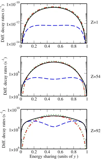
4.1 Spectral distribution of theE1M1 andE1E2 . . . 56
4.2 Spectral distribution of the 2p1/2 →1s1/2 . . . 56
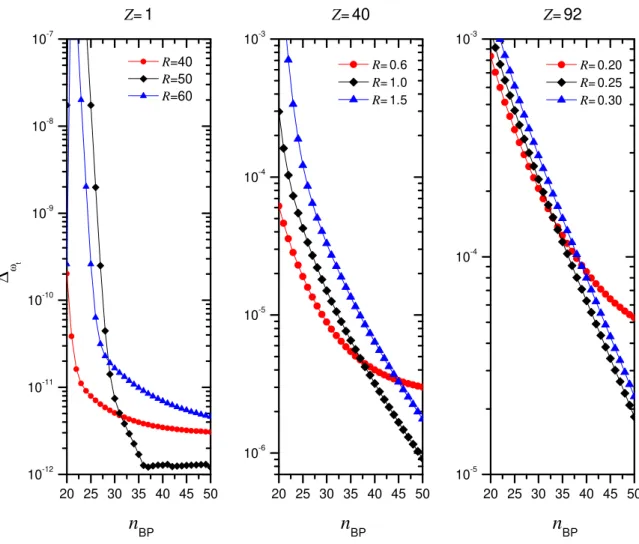
4.3 ∆ωt as function ofnBP . . . 58
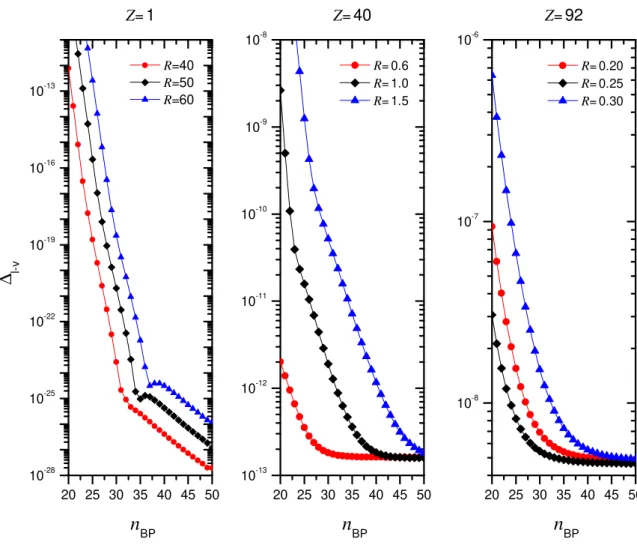
4.4 ∆l−v, as function ofnBP . . . 59
4.5 ∆l−vin double and quadruple precision . . . 60
4.6 Negative contribution to the 2E1 2s1/2→1s1/2two–photon decay . . . 62
4.7 Negative contribution to the 2M1, 2E2 andE2M1 2s1/2→1s1/2two–photon decay . 63 4.8 Negative contribution to theE1M1 andE1E2 2p1/2→1s1/2two–photon decay . . . 65
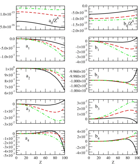
4.9 Parametersai andbi for 2s1/2 →1s1/2 . . . 70
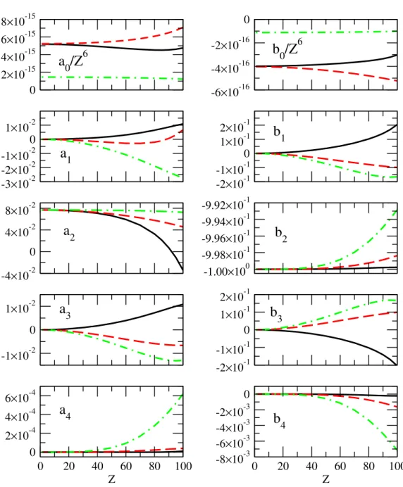
4.10 Parametersai andbi for 3d3/2 →1s1/2 . . . 71
4.11 Parametersai andbi for 3d5/2 →1s1/2 . . . 72
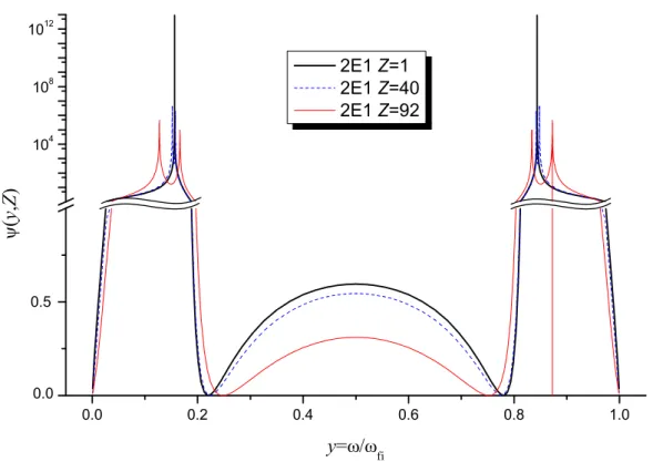
4.12 Spectral distribution of 3s1/2→1s1/22E1 . . . 76
4.13 Transparencies of 3s1/2→1s1/2 . . . 78
4.14 Spectral distribution of 3d3/2→1s1/22E1 . . . 79
4.15 Spectral distribution of 2p3/2→1s1/2 E1M1 . . . 80
4.16 E1M1 Multipole contribution of 2p3/2→1s1/2 . . . 83
6.1 Simple DCS representation . . . 104
6.2 SIMPA’s ECRIS representation . . . 105
6.3 Concept of the rotating table . . . 107
6.4 Spectrometer setup . . . 108
6.5 Image of the DCS at SIMPA. . . 111
6.6 Measurement of the vertical tilt with zerotronic sensor for several horizontal angles. . 112
7.1 Bragg and Laue diffraction types . . . 115
7.2 Reflectivity obtained from XOP . . . 116
7.3 Geometry of the DCS in an horizontal plane . . . 118
7.4 Geometry of the DCS in a vertical plane. . . 119
7.5 FunctionG(ϑ, φ). . . 121
7.6 Optical axis . . . 127
7.7 Flowchart of the simulation . . . 128
7.8 Simulated parallel rocking curve . . . 134
7.9 Simulated antiparallel rocking curve . . . 135
7.10 Energy obtained for several values of vertical misalignment . . . 139
7.11 Simulation of the energy done for several values of crystal tilts . . . 140
7.12 Simulation of the parallel peak done for several values of crystal tilts and vertical misalignment . . . 142
7.13 Simulation of the parallel FWHM done for several values of crystal tilts . . . 143
7.14 Simulation of the energy done for several values of crystal tilts and vertical misalignment144 7.15 Simulation of the antiparallel shift done for several values of first crystal angle . . . . 145
7.16 Simulation of the antiparallel amplitude done for several values of first crystal angle . 146 7.17 Horizontal slice of a bent crystal . . . 147
7.18 Simulated parallel rocking curves with bent crystals . . . 148
7.19 Parallel FWHM with a bent crystal for several values of first crystal angle . . . 149
7.20 Simulation of FWHM done for several curvature values . . . 150
8.1 Measured parallel rocking curve . . . 155
8.2 Measured antiparallel rocking curve . . . 156
8.3 Measured parallel peak position . . . 158
8.4 Parallel FWHM of measured rocking curves . . . 158
8.5 Parallel rocking curve for first crystal angle of -129.17o . . . 159
8.6 Parallel FWHM of measured rocking curves . . . 159
8.7 Parallel spectrum . . . 160
8.8 Temperature at different parts of crystal and support . . . 160
8.9 Experimental antiparallel rocking curve . . . 161
8.10 Antiparallel spectrum . . . 162
8.11 M1 transition energy . . . 164
A.1 Crystal internal structure . . . 190
A.2 Unit cell diamond cubic structure . . . 191
A.3 Miller planes . . . 192
A.4 2d simple representation of a crystal structure . . . 192
B.1 Simulation graphical input . . . 199
List of Tables
3.1 Classification of one electron orbitals in H-like ions . . . 16
3.2 Energies obtained from finite basis set method . . . 38
3.3 Coefficientsa0j anda1j . . . 48
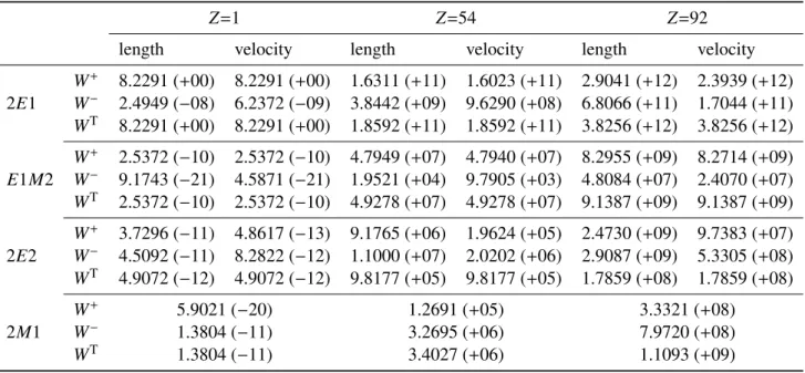
4.1 Multipole contributions for the 2p1/2→1s1/2 . . . 54
4.2 Two-photon decay rate of non-resonant states . . . 55
4.3 Multipole contributions for B-Polynomials and B-splines . . . 61
4.4 Contributions of the positive and negative energy to several multipole contributions . 66
4.5 Two-photon with B-polynomials and B-splines . . . 67
4.6 Parameteraifor 2s1/2→1s1/2 . . . 69
4.7 Parameteraifor 3d3/2→1s1/2 . . . 73
4.8 Parameteraifor 3d5/2→1s1/2 . . . 73
4.9 Parameterbifor 2s1/2→1s1/2 . . . 74
4.10 Parameterbifor 3d3/2→1s1/2 . . . 74
4.11 Parameterbifor 3d5/2→1s1/2 . . . 75
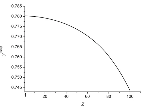
4.12 Transparencies for several two-photon transitions . . . 77
4.13 Radiative corrections . . . 78
4.14 Sum ofhLPAandhLPA1 . . . 81
4.15 Sum ofhTLAandhTLA
1 . . . 82
4.16 Multipole contributions for the 2p3/2→1s1/2 . . . 83
4.17 Multipole contributions for the 3s1/2 →2s1/2 . . . 84
4.19 Two-photon non-resonant correction . . . 86
4.20 α0for transitionsns→n′sandZ=1 . . . . 89
4.21 α0for transitionsns→n′sandZ=54 . . . 90
4.22 α0for transitionsns→n′sandZ=92 . . . 90
4.23 α0for transitionsns→n′pseveral atomic numbers . . . 91
4.24 Two-photon decay rate for the transition 1s2s1S0→1s2 1S02E1 . . . 93
8.1 Parameters after fit . . . 157
8.2 Experimental uncertainty . . . 163
Nomenclature
Vector notations
• Symbols in bold represents vectors, e.g.,pin pag. 12.
• Bold symbols with a circumflex hat are unitary vectors, e.g.,ˆkj = kj
|kj| in pag. 23.
List of Variables
The following list of themostused variables are sorted by order of appearance. A given symbol can
have a different meaning if defined in a particular part of the text not related with the global definition.
Z Atomic number Pag. 1
ni(f) Initial (final) quantum principal number in one-electron orbitals Pag. 7
ji(f) Initial (final) angular momentum in one-electron orbitals Pag. 7
c Light speed Pag. 12
p Momentum operator Pag. 12
α Dirac Matrices Pag. 12
A Vector potencial Pag. 13
HD One electron Dirac hamiltonian Pag. 13
V(r) Nuclear potencial Pag. 13
Ylm Spherical harmonics Pag. 14
li(f) Initial(final) orbital momentum in one-electron orbitals Pag. 14
Pnκ Large radial component Pag. 15
Qnκ Small radial component Pag. 15
α Fine structure Pag. 16
G Gaugeparameter Pag. 23
ˆ
e Polarization vector Pag. 23
k Wavenumber vector Pag. 23
L Order of the Multipole Pag. 24
r Vector position Pag. 24
jL Spherical Bessel function Pag. 25
ω Frequency of a photon Pag. 27
Ji(f) Total initial (final) angular momentum Pag. 27
Li(f) Total initial (final )orbital angular momentum Pag. 28
Sj(2,1) Reduced two-photon matrix elements Pag. 28
W Two-photon decay rate Pag. 29
R Radius of the region defining the atom in numerical methods Pag. 31
WC Two-photon angular correlation Pag. 41
PL Degree of linear polarization Pag. 43
α0 Two-photon absorption parameter Pag. 51
DLMq Wigner rotation matrix Pag. 52
λ Photon wavelength Pag. 103
θB Bragg angle Pag. 103
d Inter-planar distance Pag. 103
θC Angle between the optical center and crystal surface Pag. 110
θF First crystal position angle Pag. 110
θT Angle between the table axis and the X-ray source optical center Pag. 110
List of Acronyms and Abbreviations
The list of the most used acronyms and abbreviations follows the order of appearance.
HCI Highly Charged Ions Pag. 1
QED Quantum ElectroDynamics Pag. 1
CI Configuration Interaction Pag. 1
RMBPT Relativistic Many Body Perturbation Theory Pag. 2
MCDF MultiConfigurational Dirac-Fock Pag. 2
DCS Double Crystal Spectrometer Pag. 4
HFI HyperFine Interaction Pag. 4
CMB Cosmic Microwave Background Pag. 7
PNC Parity Non-Conservation Pag. 8
LAPACK Linear Algebra PACKage Pag. 32
LPA Line Profile Approach Pag. 44
TLA Two-Loop self-energy Approach Pag. 44
ECRIS Electron Cyclotron Resonance Ion Sources Pag. 101
FWHM Full Width at Half Maximum Pag. 105
Forbidden Transitions
In atomic physics, a radiativeforbiddentransition is an electronic transition between two states that is not permitted by electric dipole selection rules, i.e., it cannot occur by radiative emission of an electric dipole photon (E1). In this case, the electron decays by the next allowed multipole (magnetic dipole M1 or electric quadropole E2), or by a two-photon decay (2E1). On the other hand, if the radiative emission of an electric dipole photon is possible by selection rules, then the transition is calledallowed. Another type of transition that can be classified as forbidden is an induced electric dipole transition, which only occurs when the atom is influenced by a weak perturbation, such as an applied electric field, or a nuclear magnetic moment.
Forbidden transitions were first considered in a classical paper byBreitandTeller[1], where it is shown that the 2sstate of hydrogen and the 1s2s1S0state of helium decay primarily by two-photon emission (2E1), while the 1s2s 3S1 state of helium decays by a magnetic dipole transition (M1). These forbidden transitions have very low transition rates in neutral or few-ionized atoms compared with the rates of the allowed ones. A state that has a forbidden transition as the main decay channel, is known as a metastable state due to it’s long lifetime. However, for ions with few electrons, the decay rate of allowed transitions scales approximately with the atomic number asZ4 compared with the scaleZ6−Z10of these forbidden transitions, which makes them comparable for highly charged ions (HCI).
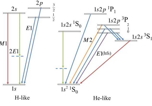
In Fig. 1.1 it is shown an overview of allowed and forbidden transitions between energy levels in H-like and He-like ions. In the case of He-like ions, the latest values of the energy levels are given in Refs. [2, 3], while for H-like the latest values can be found in Ref. [4]. These energy levels were obtained considering both relativistic, quantum electrodynamics (QED) and many-body effects (for
He-like ones).
The evaluation of the many-body effects, or the electron-correlation, is performed using the
1
s
2
s
M
1
2
E
1
2
p
3 21 2
E
1
1
s
21
S
0
3
S
1
1
s
2
s
1
S
0
1
s
2
p
1
P
1
1
s
2
p
2 1
0
3
P
1
s
2
s
M
2
E
1
(hfs)
H-like
He-like
Figure 1.1: Allowed and forbidden transitions in H-and He-like ions- Each arrow represents a transi-tion between two states. Only initial orbital states lower than three (ni<3). On each transition is labeled the most dominant decay channel. In case of the transition 2s→1sthe 2E1 is dominant for lower values
of atomic number, while theM1 is dominant for higherZ’s. The multipole terms have the colors according
to: blue-E1; red-M1; green- 2E1; orange-M2; purple- E1 (HFI). If the dominant multipole term of the
transition is anE1 then the transition is allowed, otherwise is forbidden.
method (RMBPT) [6], or the multiconfigurational Dirac- Fock (MCDF) method [7, 8, 9]. These methods share the same main features: their treatment is based on the no-pair Hamiltonian and the electron correlation is taken into account within the Breit approximation. Exact relativistic effects are
provided by using the Dirac equation for each electron orbital (cf. Sec. 3.1). QED theory deals with energy corrections for several physical quantum fluctuations (cf. Sec. 3.2).
The 2sstate in H-like ions decays by a magnetic dipole transition (M1) or by a two electric dipole transition (2E1) to the ground state. These decay rates scale approximately as 2.50×10⁻⁶Z10s−1[10] and 8.226Z6s−1[1], respectively. For lower values ofZ, the 2E1 rate dominates theM1 rate, they are equal at approximatelyZ=41 [11, 12], and for higher values ofZthe main decay channel is theM1.
photon decay is possible due to selection rules (cf. Sec. 3.3.1), which forbids Ji = 0 → Jf = 0
single-photon transitions. Therefore, the two-photon decay is necessarily the main decay channel,
which is similar to the H-like case. Since the 1selectron does not participate in the transition but acts
as a spectator, it shields the nuclear charge for the active electron. This decay scales approximately
as 16.45×(Z−σ)6 s−1, withσbeing a shielding parameter. Accurate values of this decay and the
most recent measurement can be found in Refs. [14, 15].
The 1s2s3S1state also exhibits a M1 decay to the 1s2 1S0ground state, as first established from
astrophysical observations [16]. Gabriel and Jordan emphasize the importance of this decay, by
relating its decay rate with the electron density in the solar corona [17]. This transition rate scales
approximately withZas 1.66×10⁻⁶×Z10s−1and precise values can be found in Ref. [18, 19, 20].
The states 1s2p3P2,1,0decay by anE1 transition to the 1s2s3S1. The state 1s2p3P2also makes
aM2 forbidden transition to the ground state, as pointed out byMizushima[21]. These calculations
were extended by Garstang to spectral lines of interest in the de-excitation of atoms in the solar
corona [22]. This rate scales asZ8, and already at He-like Ar (Z = 18) the M2 andE1 decay modes
are equally probable. This is a rare circumstance in atomic physics, where a M2 decay dominates
over anE1 decay channel. Because of the spin-orbit interaction the wave functions of the 1s2p3P1
and 1s2p1P1 are mixed, opening the spin-forbiddenE1 decay 1s2p3P1 → 1s2 1S0. This transition
is also useful in the determination of the electron densities in the solar corona [17]. When the nuclear
spinI differs from zero and the total angular momentum, F (F = J +I), is equal to I for the state
1s2s3P0, then the latter state mixes with the 1s2p3P1. Thus, E1 transitions of 1s2p3P0 →1s2 1S0
are possible due to hyperfine interaction (HFI). This HFI significantly shortens the 1s2p3P0lifetime
[23, 24].
A more detailed description of forbidden transitions can be found in the classical review ofMarrus
andMohr [25], while a recent review related with forbidden and allowed transition lifetimes was
Having made a general description of several forbidden transitions in H- and He-like ions we now describe the objective and organization of this Thesis.
• Part I is devoted to the theoretical evaluation of two-photon transitions in H-like ions, which
have higher transition rates in forbidden transitions. Several physical effects are analyzed, being
stressed the importance of relativistic and nondipole effects in this kind of decay channel.
• In Part II I describe the experimental work done to perform an energy measurement of a
Introduction to Two-Photon Transitions
Somewhat analogous to single-photon processes, two-photon emission can be spontaneous or stim-ulated, whereas two-photon absorption is only stimulated. However, since each photon carries one unit of angular momentum in the dipolar approximation, certain transitions between atomic energy levels, forbidden in single-photon processes, are allowed in two-photon processes. Another important distinction lies in the fact that the spectrum of spontaneous two-photon processes is continuous un-like the spectrum in the single-photon processes. A continuous spectrum is possible because energy conservation requires only that the sum of both photon energies equals the energy of the transition. For the
(ni,ji)→
nf,jf
+ω1+ω2 (2.1)
transition in H-like ions, where (ni,ji) and
nf,jf
denote the quantum numbers that identify the initial and final states, respectively, andω1 andω2are the energies of each photon, the conservation of the energy states leads to the condition
Ef −Ei=ω1+ω2, (2.2)
whereEi andEf are the energies of the initial and final states, respectively.
radiation escaping from the interaction with matter. Recently,ChlubaandSunyaev[31] revived the astrophysics interest in two-photon transitions1.
Most of todays two-photon studies are focused on the determination of fundamental constants, such as the Rydberg constant [32, 33], measurement of the Lamb-shift [33, 34], in testing Bell’s inequality [35, 36], in molecular spectroscopy [37], tissue imaging [38] and protein structure analysis [39].
Another interest in two-photon transitions relies on the study of parity non-conservation (PNC) in H-like and He-like ions [40, 41, 42, 43, 44, 45, 46]. Parity non-conservation or parity violation in an atom or ion, follows from theStandard Model, which describes, among others, the electroweak interaction between leptons and nucleons. This effect was predicted by Weinbergand Salam[47, 48], and first-time evaluated for the case of atoms or ions by M. A. Bouchiat and C. C. Bouchiat [40, 41]. PNC consists in states of different parity being mixed due to the interaction of the electron
and the nucleus, mediated by the exchange of a virtual neutral massive particle, called Z-boson. Therefore, the mixed states have no define parity. The level of mixing is very small and depends on two factors: the amount of overlap of the electron wavefunction with the nuclear wavefunction and the energy difference between two adjacent states of opposite parity. For example, the two-photon E1M1 2p1/2 → 1s transition in H-like ions plays the role of the basic transition, while the parity-violating 2E1 transition becomes admixed by PNC electroweak interaction [42]. Moreover, in recent years, two-photon transitions in heavy He-ions have attracted much attention as a promising tool for studying atomic PNC effects [45, 46]. In He-like heavy ions the overleap between the electron and
nuclear wavefunctions is a sizable fraction of the nucleus and the two levels 1s2p3P0and 1s2s1S0 happens to be almost degenerate forZ= 64 (gadolinium) and 90 (thorium), thus enhancing the PNC
effects significantly [43].
The possibility of forbidden two photon transition, Ji = 1 → Jf = 0 with two equal energy
sharing being induced by HFI was considered as a possible route to measure violations in Bose-Einstein statistics [49, 50].
The two-photon spectral distribution of the 2s → 1stransition in H-like ions has recently been used for precise efficiency calibration of solid-state X-ray detector as it has a known shape for a large
distribution of energies [51].
From a theoretical point of view, the 2s→1stwo-photon transition rate in H-like ions has been calculated and discussed many times using different approaches. An historical overview from both
theoretical and experimental point of view can be found in the article bySantos et al. [12]. In that work, B-splines basis set techniques were applied to the evaluation of two-photon amplitudes based on the Dirac equation and were discussed relativistic and non dipolar effects. Meanwhile, a similar
1A review of the Cosmological Recombination Epoch and the role of the two-photon decay can be visualized in this
Green’s function [52].
In the non-relativistic framework, other transitions were studied, for instance, byTung et al.[53] andKlarsfeld [54], who performed calculations for transitions from an arbitrary state (ni,li) to an
arbitrary state (nf,lf). Florescu et al. [55] developed a theory for two-photon transitions in H-like
systems, including the 3s→1sand 3d→1stransitions.
The first relativistic inner-shell calculation of two-photon for bound states was made byMuand
Crasemann[56] followed byTong et al. [57]. Surzhykov et al. [58] performed another relativistic
calculation to study the angular correlations in the two-photon decay of H-like ions.
Recently, Labzowsky et al. [59] evaluated the 2E1 contribution for the 2s → 1s transition and theE1M1 andE1E2 contributions for the 2p1/2 →1stransition. They derived an expression similar to the one obtained by GoldmanandDrake [60] in the QED framework. Also in this framework,
Nganso et al.[61] carried out the treatment of theS matrix for bound-bound transitions.
The 1s2s1S0 → 1s2 1S0 two-photon decay in He-like Tin was recently measured byTrotsenko
et al.[15] using a novel method of populating the 1s2s1S0based in relativistic collisions of Li-like projectiles with low-density gas. The high statistics and accuracy inherent to the method enabled the observation of relativistic effects for the first time.
Also this two-photon decay rate in He-like have been recently calculated byVolotka et al.[62] with the inter-electric interaction evaluated within the QED framework of the two-time Green func-tion.
The use of polarization correlations properties of the emitted two-photons was recently considered byFratini et al.as a route for measuring atomic PNC and studying entanglement correlations [63, 64].
As for two-photon absorption or excitation, a series of highly accurate measurements has been performed on two-photon excitation of neutral hydrogen and deuterium atoms [33, 65, 66, 67], which reveal QED effects and determine the Rydberg constant and Lamb-shift with a record accuracy. Apart
in the infrared, visible, and ultraviolet regime, recently, it was observed for the first time byDoumy et al.in the X-ray regime [72] using an highly intense X-ray Free-Electron Laser (XFEL).
Recent technical advances in polarization and position-sensitive detectors have opened up the possibility of investigating angular and polarization properties of the radiation emitted in atomic decays [73, 74]. It is foreseen measurements of two-photon angular correlations will be therefore performed, within the near future, at GSI in Darmstadt [75, 76], which will test quantum correlations of the photon pair [63] and PNC in He-like ions [64].
After I made an introduction to this kind of transition in atomic physics, the rest of this part is organized as follows: in Chapter 3 we give a review of the background theory involving in a two–photon emission, which also includes numerical methods necessary for the evaluation of the re-duced two-photon amplitudes. In Chapter 4 we present the results obtained in this work. Several physical effects in a two-photon decay, such as resonances, the negative continuum contribution and
Theory of Two-photon Transition
Since all the evaluations in this work were done in a relativistic framework of the Dirac equation, this equation is presented in Sec. 3.1 along with a description of the relativistic effects of an electron in
an HCI nucleus. Then, we make a description of the formalism necessary for deducing two-photon properties in Sec. 3.2 and apply it to the case of spontaneous two-photon emission in Sec. 3.3.
Afterwards, we describe some numerical methods for evaluating the reduced two-photon ampli-tudes in Sec. 3.4. Emphasis will be done to thefinite basis setsince it was the method used in the work. Along with the well-stablishedB-splinesbasis set, we introduce a novel basis set, so-called
B-polynomials. The method presented in this section was published in Ref. [77].
The method offinite basis setenables the separation of the negative-energyintermediate states from the summation over the Dirac spectrum, which is present in second order perturbation expres-sions, such as two-photon decay rates. Therefore, in Sec. 3.5, special attention is paid to the effects
on the two-photon transition rates arising from removing these states. Expressions of semi-relativistic estimates of the negative continuum contribution, published in Ref. [78], are presented in this section.
The angular correlation between the two photons are consider in Sec. 3.6. In particular, the expressions for the angular correlation are expanded in terms of cosθ-polynomials, whose coefficients
depend on the atomic number and the energy sharing of the photon pair. The work presented in this section is in manuscript form for publication.
In Sec. 3.2 we consider the physical changes betweennon-resonant andresonanttransitions in the two-photon emission. While the former type has no real intermediate states between the final and initial state of the decay, like the 2s1/2→1s1/2transition, in the resonant transitions, the two-photon transition has also a decay channel related with the cascade one-photon de-excitation process. The theoretical discussion was published in Ref. [79].
known as two-photon absorption. The theoretical description of this section is given in Ref. [80].
In all the theoretical description presented in this chapter, it was used atomic units. A brief description of those units can be found inSantos’sThesis [81].
3.1
One electron Dirac equation
Relativistic Quantum Mechanics can be found in several textbooks [82, 83, 84, 85]. In this section, we restrict to a brief description and further details can be traced back to the references already mentioned.
3.1.1 Free electron
The relativistic invariant equation that describes the dynamic of a single electron, was obtained by Diracin 1928 [86, 87]. At that time,Diracwas searching for a relativistic invariant wave equation of the Schr¨odinger form with a positive-defined probability density. Back then, there were doubts con-cerning the Klein-Gordon equation [88, 89], which were obtained in a similar way of the Schr¨odinger equation, setting the HamiltonianHof a free electron, as
H2ψ=(c4+c2p·p)ψ=−∂ 2ψ
∂t2 . (3.1)
Herep=−i∇is the momentum operator andcis the light speed (in atomic unitsc=137.03599911 [90]). Such approach did not yield a satisfactory probability density, since it can have both positive and negative values. A reason of this fact is that the Klein-Gordon equation is of second order in time. Diracproposed that the Schr¨odinger-like equation of the free electron motion, which is linear in time, should also be linear in the spatial components. Hence, Dirac proposed that the dynamic of a single free electron obeys the equation
i∂ψ
∂t =(−icα·∇+c
2β)ψ . (3.2)
The coefficientsαandβmust not be simple numbers, otherwise these coefficients define a direction
for the partial derivatives and this equation will not be invariant with respect to spatial rotations. To overcome this problem, those coefficients can be defined as square matrices, and hence, the
wave-function as column matrices. By doing so, Eq. (3.2) becomes a system of linear first-order differential
It also restricts the dimension of those matrices to an even number greater than three. One possible representation, among others, is given by
α= σ0 σ0
, β=
0I 0
−I
, (3.3)
whereα andβare known as Dirac matrices. The cartesian components ofσare the Pauli matrices
andIis the unitary matrix given by
σx =
01 10
, σy=
0i −0i
,
σz=
10 −01
, I = 10 01
.
(3.4)
By doing so, it can also be demonstrate that the particle density,ψ†ψ, follows the continuity equation
and Eq. (3.2) is invariant to a Lorentzian transformation [83].
3.1.2 One electron in a nucleus potencial
In case the electron being immersed in an external electromagnetic field, the electromagnetic interac-tion is included in the Dirac equainterac-tion using theminimal coupling[91],
E → E−V ,
p → p− A
c . (3.5)
This substitution assures not only gauge invariance of the Maxwell equations, but also a Lorentz force acting on the electron. Eis the free electron energy,V is a scalar potential andAis the vector
potential. Thegaugetransformation is defined by
A′(r,t) → A(r,t)+∇ϑ(r,t), (3.6)
and is a consequence of charge conservation. ϑis an arbitrary function, that keeps the electrical and magnetic fields invariant to that transformation.
If the external electromagnetic field is due to the nucleus of an atom then an additional term,V(r), is included next toc2βin Eq. (3.2), i.e.,A=0andV =V(r).
i∂ψ ∂t =
h
The termV(r) is the radial potential of the nucleus and is given according to the nucleus model used. In case of a point nucleus model, it is given by the well-known expression of a point-like source Vp(r) = −Z/r, where r is the distance to the nucleus and Z the atomic number or the number of protons. The next upgrade of this simple model is considering the nucleus as a uniform distribution of charges. Thus, the nuclear potential is given by
VU(r)= Z 2RN r RN 2 −3
r ≤RN
−Zr r >RN
, (3.8)
whereRNis the nucleus radius given by
RN =2.2677×10⁻⁵ 3 √
A, (3.9)
where in this case,Ain Eq. (3.9) is the atomic mass number. Other charge density of the nucleus can be considered, for instance a Fermi distribution [4]. All the evaluations done in this work were done using a nucleus uniform distribution (Eq. (3.8)) and a point nucleus was used only for comparison with analytical results based in that approximation.
Those spherical potentials (e.g. Eq. (3.8)) does not depend on time, so we can use the stationary version, HDψ = Eψ. Because of the spherical symmetry of the potential, the square of the total angular momentum,j = l+s, and the relativist parity operator,Π =eiϕβ(r → −r) commutes with
Dirac Hamiltonian. Thus, as in the case of the non-relativistic Schr¨odinger equation, the wavefunction consists of a product of the angular part, which depends on the direction of the vector position,rˆ, and
a radial part that depends onr=|r|. Furthermore, the angular part is an eigenfunction of thej2, jzand
Π. Following the angular quantum rules of combining two angular momentum operators to form a
third, the spherical spinor is made by combining spherical harmonics,Yl,m, which are eigenfunctions
ofl2 andlz, and spinors, which are eigenfunctions ofs2andsz. Those spherical spinors are defined
by [92]
Ωjlm=
mXs=1/2
ms=−1/2
l m−ms,
1 2 ms
j m
Yl,m−ms(rˆ)χms . (3.10)
Here the two spinor χms (ms = 1/2, −1/2), are eigenfunctions of the spin operators
2 = σ2/4 and
Sz=σz/2. They are given explicitly by
χ1 2 =
10
, χ−1
2 =
01
. (3.11)
The eigenvalues equations, already refereed for the spherical spinor, are given by
j2Ωjlm = j(j+1)Ωjlm, jzΩjlm =mΩjlm,
The spherical spinors are also eigenfunctions ofK=1+σ·LandΠ, with eigenvalues
κ=
−l(l+1) ifif jj==ll−+11//22 , (3.13)
and (−1)l, respectively. The values in Eq. (3.13) can be summarized asκ=
∓(j−1/2) forj=l±1/2. The values ofκdetermine both jandl. Consequently, a more compact notationΩjlm = Ωκmcan be
used. By making the following ansatz for the stationary Dirac equation,
ψ= 1 r
QiPκ(r)Ωκm
κ(r)Ω−κm
, (3.14)
we may eliminate the angular part in both sides of the equation and obtaining the differential equations
for the radial functionsPκ(r) andQκ(r),
V(r) c d
dr −
κ
r
−cdrd + κr V(r)−2c2 PQκ(r)
κ(r)
=(Enκ−c2)
PQκ(r)
κ(r)
. (3.15)
V(r) can be any spherical potential andǫκ= Eκ−c2is defined in order to compare with non-relativistic
energies. In fact, by expanding Eq. (3.15) in powers of 1/cand by retaining only the first term, we obtain the radial Schr¨odinger equation applied toPκ(r) withκ(κ+1)=l(l+1) and
Qκ(r)≃ − 1 2c d dr + κ r !
Pκ(r). (3.16)
Therefore, since Pκ(r) and Qκ(r) are equal to the non-relativistic radial wavefunction and zero for
c→ ∞, respectively, they are called the large and small components. If in some numerical method, the
large and small components are restricted by Eq. (3.16), they are refereed to bekinetically balanced. The normalization condition of the wavefunctions for the large and small components is given by
Z ∞
0 h
Pnκ(r)2+Qnκ(r)2
i
dr=1. (3.17)
Orbital 1s1
2 2s12 2p12 2p32 3s21 3p12 3p23 3d32 3d52
n 1 2 2 2 3 3 3 3 3
κ -1 -1 1 -2 -1 1 -2 2 -3
j 12 12 12 32 12 12 32 32 52
l 0 0 1 1 0 1 1 2 2
Parity 1 1 -1 -1 1 -1 -1 1 1
Table 3.1: Classification of one electron orbitals in H-like ions- The bound states of the electron, or orbitals, are classified according to the quantum numbersnandκ. The quantum numbers jandlare given
according Eq. (3.13). The parity is equal to (−1)l. The next letter forl=4 is f.
by Dirac [93], assuming that all the states of negative energy are occupied with electrons. In this interpretation, the vacuum is defined by the absence of real electrons in bound states and positive energy states, and all the negative energy states filled with electrons. This vacuum is sometimes refereed as the Dirac sea. Because of the Pauli exclusion principle, which forbids two particles of half spin with the same quantum numbers being at the same state, that decay it is not possible, and hence making the lowest energy bound state also the ground state. On the other hand, the electron of negative energy can absorb a photon with energy greater then 2c2and excite for a state of positive energy. The hole behaves like an electron with the same mass, spin and opposite charge and was named positron. The positron was experimentally observed in 1933 by Carl D. Anderson [94] and made it’s discovery, the antiparticle of the electron, one of the greatest triumphs of theoretical physics.
The eigenvalues,ǫnκ, of the bound states obtained after solving the eigenvalue equation (3.15) are given by the Sommerfeld formula
ǫnκ = c2
1 s
1+ (αZ)
2
n− |κ|+ pκ2−(αZ)2
−1 , (3.18)
n = 1,2,3, ... ,
l = 0,1, ..., n−1,
κ = ± j+ 1
2 !
=±1,±2,±3, ... ,
where a point-like of the nucleus was used for the spherical potential. Theαvalue is the fine structure constant, which in atomic units is α = 1/c. This energy levels only depends on |κ| and n, as a consequence of the spherical potential. Consequently, these numbers are the necessary quantum numbers for describing an one-electron state or an orbital. In Table 3.1 is shown the nomenclature used for describing one-electron orbitals.
samenandlbut different values of j, such as the 2p1/2 and 2p3/2 orbitals, have different energies. The separation between two such levels is called fine structure interval, which can be observed in Fig. 1.1. Furthermore, the degeneracy between the 2s1/2and 2p1/2could be lifted if the QED effects are considered (Lamb-shift). Usually the subscript j=1/2 in thes1/2 orbitals are omitted since it is always 1/2.
ForαZ>1, Eq. (3.18) becomes imaginary, which indicates that there is no bound states for those atomic numbers. This is due to the energy of the 1s1/2 being embedded in the negative continuum ǫnκ < −2c2forαZ >1 in a point-like nucleus model. As in theKlein paradox[83], this phenomena can be understood in the framework of the hole theory as electron-positron pair creation at the po-tential barrier. It becomes energetically favorable for the electron-positron pair not recombining, and thus, emitting a positron.
For lower values ofαZ, Eq. (3.18) can be expanded as
ǫnκ =−
Z2 2n2
"
1+(αZ) 2
n 1 κ −
3 4n
!#
, (3.19)
where the first term represents the Bohr formula for the electronic energy levels calculated according to the Schr¨odinger equation, which scales asZ2. Accordingly, relativistic corrections for the energy levels are of orderα2Z4. These corrections are significantly for small principal quantum numbers and in HCI. Moreover, the radial electron distribution shifts towards the nucleus if the Dirac equation is considered rather than the non-relativistic Schr¨odinger equation.
Having made a description of the one-electron Dirac equation, we will give a brief description of the QED formalism necessary for obtaining the two-photon expressions.
3.2
QED
QED can be found in several textbooks [82, 83, 85]. In this section, we restrict to a brief description and further details can be traced back to the references already mentioned. As refereed previously, the Lamb-shift is an energy shift between the 2s1/2and the 2p1/2. This splitting was first discovered byLambandRetherford in 1947 using precise microwave absorption techniques [95]. Since it was done for hydrogen, the effect of the nuclear model was too small to explain this splitting. This lead
to believe that these effects could be due to quantum fluctuations in the electromagnetic field or
a) b)
Figure 3.1: Self-energy and vacuum polarization Feynman diagrams- a) is refereed to the self-energy diagram while b) is the vacuum polarization diagram. The straight double line represents a bound electron and the oscillating line a photon
Calculations in QED are done in perturbative theory of the fine structureα. The terms of this perturbative expansion can be represented by Feynman diagrams. The first terms of the expansion, that gives the main contribution of the Lamb-shift, are the self-energy and the vacuum polarization terms. In Fig. 3.1 is shown a representation of these diagrams. The vacuum polarization corresponds to the interaction of the bound electron with an electron-positron pair, which is a quantum fluctuation of the Dirac sea.
The QED corrections on the atomic energy levels can be divided in one-electron corrections, where these fluctuations affects each electron independently, and two-electron corrections, which
affects the interaction between two electrons. Self-energy and vacuum-polarization [97, 98] are
one-electron corrections that gives the main contribution to the Lamb-shift. Other one-electron cor-rections, with less contribution to the Lamb-shift, are the two-loop self-energy [99] and two-loop vacuum-polarization [100]. A recent review can be found in Ref. [101]. As for the two electron cor-rections, they are calculated within the two-time Greens function [102] formalism, which evaluates the vacuum-polarization screening correction [103], the two-photon exchange correction [104], as well as the self-energy screened by a spherically symmetric part of the electron-electron interaction [105].
3.2.1 S Matrix in interaction representation
the framework of perturbation theory.
In this representation, the state vector is expressed by
Φ(t)=S(t,t0)Φ(t0), (3.20)
whereΦ(t0)= Φ(t=t0) andS(t,t0) is an operator defined by [85]
S(t,t0) = ∞ X
n=0 (−i)n
n! Z t t0 Z t t0 Z t t0 ... Z t t0
ThVI(t′1)VI(t2′)VI(t3′)...VI(tn′)
i
dt′n....dt3′dt′2dt′1
= T
e−i
Rt
t0V(t′)dt′
=
∞ X
n=0
Sn(t,t0), (3.21)
with
Sn(t,t0)= (−i)
n n! Z t t0 Z t t0 Z t t0 ... Z t t0
ThVI(t1′)VI(t2′)VI(t′3)...VI(t′n)
i
dt′n....dt′3dt′2dt′1. (3.22)
The Dyson chronological operatorT is defined by
T[V(t1)V(t2)]=
VV((t1t2))VV((t2t1) if) if t1t1<≥t2t2
. (3.23)
The operatorS(t,t0) is called the Scattering matrix, or simply S matrix. It operates on the initial state vectorΦ(t0) and the result is the stateΦ(t) at an instantt.
3.2.2 Quantified field
There are two formalisms for defining a quantum system in QED. One of such formalisms defines the system Hamiltonian through de use of path integrals and a variational principle that identifies the stationary paths of a classical system1. The other approach, which is equivalent to the last one, defines a field for a given particle which is thequantumof the field2. According to this concept, the ground state of a field is the vacuum, while an excitation of the field corresponds to a particle creation. In the case of the electromagnetic field, it consists in the electromagnetic field quantification, in which the four-vector potencialAµis expanded in plane waves of polarityeˆand wavenumberk. A plane wave corresponds to a solution of the Maxwell equations without charges. The expansion coefficients are
defined not as numerical quantities, but rather as unitary operators that can be identified as creation or destruction of a single photon with polarityeˆand wavenumberk[85]. As for the electron case,
it consists in the electron-positron field quantification, i.e., in the expansion of the functionsψand
1Developed byFeynman[106, 107]
ψthat satisfies the Dirac equation (3.7). Like in the case of the electromagnetic field, the expansion coefficients corresponds to the creation or destruction of an electron or positron.
The commutation relations of these operators are constructed in such way that the each field follows a given statistics. In the case of the electromagnetic field, the photons obey the Bose-Einstein statistics, i.e., the number of particles in a given state is arbitrary. On the other hand, the electrons and positrons obey the Pauli exclusion principle and follow the Fermi-Dirac statistics; a state contains only zero or one particle.
Using this principles, it can be deduced that the interaction operator between the electromagnetic field and the electron-positron field is given by [85]
V(t)= Z
jµ(x)Aµ(x)dV, (3.24)
whereA(x) is the four-vector potential andj(x) is the four-vector electron flux defined by
jµ(x)=iN
ψ(x)γµψ(x)
, (3.25)
whereNis an operator that sorts the operators in order to the creation operators being at the right and the destruction ones to the left. It also multiplies by one or minus one for an even or odd number of switches. Here,xis the space-time four-vector (r,−it).
Using the Eqs. (3.24) and (Eq. (3.25)), the matrixS can be rewritten as
S(t,t0) = ∞ X
n=0 (−i)n
n!
Z Z Z ...
Z
T[U(x1)U(x2)U(x3)...U(xn)]d4xn...d4x3d4x2d4x1
= T
" exp(−i
Z
U(x)d4x)
#
, (3.26)
where
U(x) = −iNψ(x)γµAµ(x)ψ(x)
=−iNψ(x) ˆA(x)ψ(x) . (3.27)
A given interaction mode between the electromagnetic field and the electron-positron is an pro-cess if the matrix S is proportional toαn. In this way, anprocess is described by the matrixS
n(t,t0).
Here ˆA(x)=γµAµ(x) andψ=ψ∗β.
i i f
f k
2eˆ2
k
1eˆ1 k2eˆ2
k
1eˆ1
Figure 3.2: Two-photon transition Feynman diagrams- Representation of the Feynman diagrams for an emission of two photons with polaritieseˆ1andˆe2, and wavenumberk1 andk2. The two diagrams
corresponds to the two permutations of the two photon creation operators.
from an initial state to a final state by spontaneous emission of two photons, one of the annihilation operators must annihilate the electron in the initial state and three creation operators creates one electron and two photons in the final state. All the other operators must join in creation-annihilation pairs of the same particle (electron, positron or a photon). A Feynman diagram of this process is illustrated in Fig. 3.2. The thin lines that goes from infinite to a vertex, are operators that create or destroy an electron. The thick line corresponds to compacting all the creation-annihilation pairs of the same particle. The oscillatory line is a destruction or a creation of a photon.
3.2.3 S Matrix for two-photon transition
Thenorder matrix S of a processi→ f is defined by
S(in→)f =DΦf|Sn|Φi
E
=X
k
Sk(n), (3.28)
whereΦis a state vector in the Fock space or particle number space. Thus, all the unitary operators
are removed. EachS(kn) term differs by the order of the creation and annihilation operators in the
same process. In the case illustrated in Fig. 3.2, the number is two due to the possible number of permutations between the two photon creation operators.
The matrix elements involved in a second order interaction between the electromagnetic field and the electron-positron field is described by the matrix S given by
S2= Z Z
ThNψ(x1) ˆA(x1)ψ(x1)
Nψ(x2) ˆA(x2)ψ(x2) i
d4x1d4x2. (3.29)
associated toS2. The matrix S for the diagram in Fig. 3.2 is given by
S(2)i→f = Z hψf(x2) ˆA∗2(x2)SG(e)(x1,x2) ˆA1∗(x1)ψi(x1)
+ψf(x2) ˆA1∗(x1)S(Ge)(x1,x2) ˆA∗2(x2)ψi(x1)
i
d4x1d4x2
= S(2)a +S(2)b . (3.30)
The statesψi(x) andψf(x) are the wavefunctions of the electron in the initial and final states, and ˆA1
and ˆA2are the wavefunctions of the photon with polarityeˆ1(2)and wavenumberk1(2).
The functionS(Ge)(x1,x2) is the mean value of the various creation-annihilation pairs of the same
particle (in this case electron and positron) resulting from the Dyson operator along with the Normal
operator. It is given by [85]
S(Ge)(x1,x2)= X n
ψn(+)(x1)ψn(+)(x2) if t1≥t2
−X
n
ψn(−)(x1)ψn(−)(x2) if t1<t2
, (3.31)
where
ψn(±)(x1)=ψn(±0)(r1)e−iE (±)
n t , (3.32)
are the solutions of the Dirac equation (3.7) for an electron in external field given by the nuclear
potential. The sum covers all the energies of the Dirac spectrum, both positive (+) and negative (−)
states. In the case of a continuous energy band, such as the positive or the negative continuum, this
sum is interpreted as an integral.
Considering the following identity [85]
1 2πi
Z ∞
−∞
eiωt
E(1−i0)+ωdω=
0 E <0 e−iEt E >0 t>0
−e−iEt E <0 t<0
, (3.33)
S(Ge)(x1,x2), known as the Green’s function, can be given in a more compact expression given by
S(ce)(x1,x2)=
1 2πi
Z ∞
−∞
eiω(t1−t2)X
n
ψn0(r2)ψn0(r1)
En(1−i0)+ω