Underwater acoustic simulations with a time variable acoustic propagation model
A. Silva, O. Rodriguez, F. Zabel, J. Huilery, S. M. Jesus
University of Algarve, Institute for systems and Robotics, Faro, Portugal, {asilva,orodrig,fzabel,jhuilery,sjesus}@ualg.pt
The Time Variable Acoustic Propagation Model (TV-APM) was developed to simulate underwater acoustic propagation in time-variable environments. Such environment variability induces a strong Doppler channel spread, which is an important factor to test and evaluate the performance of equalization algorithms. In current simulations, Doppler spread is usually included a posteriori in a stationary Acoustic Propagation Model (APM), and is designed for specific environmental parameters such as source-receiver range variability or surface motion. However, environmental variations affect Doppler spread in a complex manner, and an accurate TV-APM simulation for time varying channels, being performed at the same sampling rate as the transmitted signal, would require a large number of runs at high frequencies. A strategy in the current implementation of the TV-APM was developed to reduce the number of runs, while preserving the variable-channel Doppler spread. Simulations were done to draw a performance map for a given equalizer in a given environment and the results revealed that the TV-APM is a useful prediction tool of communication equalizers performance.
1
Introduction
The objective of this work is to develop an underwater acoustic channel simulator for use in performance evaluation of a Point to Point (P2P) communication system in a time-variable channel. The simulator can be used to evaluate the performance of communication systems over various configurations, such as different source-receiver ranges, source and receiver depths. Such information can infer configurations that provide reliable communications for that site. For that purpose the Time Variable Acoustic Propagation Model (TV-APM) was developed to fulfill the gap of simulating underwater acoustic propagation experiments in a time variable environment. The major motivation for the time-variable simulation of underwater communication experiments is due to the fact that to test and measure the performance of equalization algorithms one of the most important factors is the environmental time variability that causes a strong Doppler spread in the channel output signals.
Underwater channels are time-variant and spread both in delay and Doppler [1]. The spread in delay is usually given by the multipath that results from multiple reflections in the boundaries and refraction in the water column due to the sound speed profile. The Doppler spread results from the variable environment properties during a time window of interest. The time-varying nature of underwater acoustic propagation is driven by several phenomena at short time-scale (e.g. sea surface motion and range and depth motion of the transducers) and in a large time-scale (e.g. internal waves and tidal cycles). The short time-scale phenomena are of most interest for communications since data is usually transmitted in time windows of several seconds.
Doppler induced by a constant relative speed between the transmitter and the receiver caused a compression or expansion of the received signal and can be easily simulated. However Doppler spreading caused by up/down movements and surface waves, cannot be easily simulated [1,2]. The former can be simulated by a simple resample of the received signal while the latter needs a more elaborated approach. The most generic one is the simulation of the time varying channel Impulse Response (IR) during the data transmission followed by a time-variable convolution implementation.
Some of the applications of the TV-APM are: to study the environmental effects that most degrade a given equalizer performance, to allow the comparison between different equalization methods under similar conditions and to simulate the most appropriate geometric source-receiver configuration to attain the best performance in a given static or time-varying environment. The latter allows the drawing of performance maps for a site of interest for a given equalizer. In this paper, an environmental-based equalizer performance will be evaluated in different configurations for the region north of the Formiche di Grosseto in the west coast of Italy.
The environmental-based equalization used in this paper is based on passive time-reversal and waveguide invariant properties of ocean channels [3]. Passive time-reversal [4] allows for the implementation of a simple communication system where the Intersymbolic Interference (ISI) is mitigated by a correlation between a probe (for channel IR estimate) and the actual channel IR during data transmission. The primary cause of performance degradation of the pTR is the presence of mismatch between the probe and the data transmissions. The environmental equalizer makes use of the waveguide invariance, which states that geometric mismatch (i.e. source and array depth and range variations) can be
compensated by applying an appropriate frequency shift to the channel IR estimate [5]. For that reason it is termed Frequency Shift passive Time Reversal (FSpTR).
In section 2 it is shown that the Doppler distortion can be induced in the received signal using a time variable convolution. Section 3 briefly explains how the FSpTR equalizer can compensate for the Doppler distortion. In section 4 the strategy adopted for the Doppler-time simulation is clarified. Section 5 shows how the TV-APM can be used to draw the performance map of the FSpTR equalizer in a given site. Section 6 summarizes the main results, draws some conclusions and suggests future work.
2
Doppler distortion
The objective of this section is to show that the Doppler effect that is usually modeled as a compression/expansion of a signal can be introduced in a received signal by a time-variable convolution in base-band.
When there is a range variation caused by a constant velocity between a source and a receiver, the Doppler effect is usually associated with the compression or expansion of the signal due to the ratio between the source-receiver velocity and the sound propagation velocity. Consider that only that the source is moving and that a communication signal is transmitted with a carrier frequencyc. In such case the base-band version of the transmitted signal,x(t), can be modeled as [6]
t j D t x t e c
x () ((1)) (1)
where is the time compression/expansion factor as given by 1 / 1 1 c v . (2)
This factor depends on the ratio between the physical parameters: source velocity v and sound velocity c . In (1) the Doppler effect amounts to time scaling the transmitted signalx(t)with a factor of (1)and to frequency shifting with c.
Assuming first that there is a single propagation path, )
(t
gmp , between the source and the m -th hydrophone of
an array. The receiving signal is given by the convolution [6]
x t g d t
ymp() D( ) mp( ) . (3)
Performing a change of variable yields
d e t h c v t x t y j c mp mp() ( ) 1 (, ) ~ (4) where c v t j mp mp c e c v t g t h ) ( ~ ) ( ) , ( (5)represents a time-variable IR andtand the time and delay axis respectively.
In (4) the term in [.] represents the base-band version of a channel time-variable IR hmp(t,)and reveals that the Doppler distorted received signal can be computed with a time-variable convolution. The advantage of using (4) rather than (3) for the computation of the Doppler distorted received signal is that (4) can be easily generalized for a multipath channel since
p mp mp m t h h (,) ( ) (6)whereprepresents each path that arrives to the m -th hydrophone with delay mp and hm(t,) the multipath channel IR. Applying (6) in (4) results
xt h t d t
ym() ( ) m(, ) (7)
that represents the Doppler distorted signal received by the m -th hydrophone in a multipath channel. Since the channel IR can be modelled by an Acoustic Propagation Model (APM) with a large number of environmental properties as inputs, the time-variable convolution (7) was used in the development of the TV-APM presented in this work.
3
Environmental-based equalizer
Equalizers are used in underwater coherent communications to track channel IR and to compensate for ISI due to time varying multipath. Equalizers are usually developed based on time varying channel models which conceptually ignore the fact that IR variability is caused by fluctuations of environmental parameters. Their major drawback is that the relation between environmental properties variation and IR time variability is nonlinear, which is believed to cause frequent lack of convergence and hangups. To avoid such instability, an Environmental-based equalizer that considers that the channel mismatch compensation should take into account the time variability of environmental properties is under development [3] and its actual version is used in this work.
The FSpTR environmental-based equalizer aims at minimizing the MSE (between the transmitted and received data-stream) by taking into consideration the environmental properties that are varying during the data transmission. The FSpTR [3,7] is capable of compensating the source/receiver depth and source-receiver range variations.
The FSpTR equalizer is based on the pTR operator [4] that allows for the implementation of a simple equalizer that deconvolves the channel multipath by filtering the received data with time-reversed estimates of the channel IRs.
However, one of the pTR primary causes of performance degradation is due to source and array movement. In the FSpTR scheme a frequency shift is applied to the IRs estimate in order to compensate for environmental changes, resulting in an adaptive equalizer. Figure 1 shows (from left to right) the multipath between the source and the receiving array as well as the FSpTR operation. For the case when only the range is varying, the FspTR behavior can also be understood using (5), where it can be seen that as the time t evolves the initial IR gm(0,) gradually slides in the delay axis and is frequency shifted accordingly. In a short time scale the sliding in time can be considered approximately zero but the shift in frequency, depending ofc, can have quite a large impact on the received signal especially when coherent communications are considered. It is clear from (5) that such shift in frequency can be compensated by applying an appropriate frequency shift in the opposite direction. In [3,7] the FSpTR was shown to compensate for the range and depth channel variability and its extension to other environmental properties is now under study. The simulation results presented in section 5.2 were obtained using this equalizer.
Figure 1: Probe and data signals underwater propagation (left); Block diagram of FSpTR equalizer (right): (i) filtering of hydrophone received data with time-reversed
FS IR estimates, (ii) addition of filtered signals for each FS, (iii) selection of the FS signal with maximum power, (iv) down-sampling to the symbol rate and (v) estimate of
transmitted symbols.
4
Doppler-time simulation setup
One of the main objectives of the communication simulator is to test equalizers' performance in presence of a realistic time variable channel. Its primary concern is to model the time variability induced by node mobility and surface wave’s motion during communications. An originality of this simulator is that the Doppler spread induced by each time variable parameter is duly accounted for by using an acoustical propagation model to compute the Doppler-time distorted received signal.
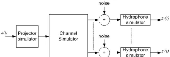
The acoustic channel simulator block diagram is shown in figure 2, where a single input multiple output (SIMO) model was considered. The full system requires the simulation of the transducers that can be represented by their frequency responses, and of the time-variable channel. The most problematic aspect of the channel simulator is the time variability since it strongly affects
performance of demodulation/equalization techniques. That implies that a time variable simulation of the acoustic channel IR and a time variable filtering implementation are required. The latter was briefly described in section 2.
Figure 2: Channel simulator block diagram
The discrete implementation of (7) requires that both
t
and
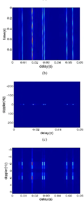
are sampled with the same sampling period. This fact imposes a serious constraint to the simulator implemen-tation since it requires the APM for channel IR simulation to be run at the sampling frequency of the communication signals, which is an extremely difficult task due to the propagation model computation time consumption and to the resulting extremely large amount of data. However, considering the frequency-dispersive characteristics of the underwater acoustic communication channel it can be shown that the required time sampling to characterize the channel time variability is much lower than that required to characterize the channel time-dispersion when used for propagating high data rate communication signals. It results that in the discrete computation of the channel IR the sampling frequency of true time t can be much lower than the sampling frequency of relative time which implies that the acoustic propagation model can be run less often than the signal sampling frequency, without compromising a faithful characterization of the channel time variability.In order to gain some insight about the time sampling requirements of underwater time-varying channels, figure 3 shows the delay-Doppler scattering functions of real IR estimates for the same channel at the same time but with different bands. The IR estimates were computed by pulse compressing 100 ms chirp signals transmitted with a 300 ms interval during 15 s, with a band of 2 kHz centered at 6 kHz in (a) and a band of 4 kHz centered at 12 kHz in (b). Figure 3(a) shows that the scattering clearly vanishes in the Doppler axis revealing that the 300 ms time sampling of the channel is sufficient to represent the time variability of the channel. In fact, since the scatters vanish at +1 and -1 Hz the channel sampling could be reduced to 0.5 s. Figure 3(b) shows that the scattering do not vanish in the axis length (between -1.67 and +1.67) revealing that for a correct representation of channel variability the channel time sampling should be increased to 250 ms.
Figure 4 shows an example of IR simulation with source movement. Figure 4(a) shows the time-delay IR where only the source-range and hydrophone depth vary along the time axis. In the time axis the channel is sampled at 501 Hz while in the delay axis there are 7 distinct channel paths.
(a)
(b)
Figure 3: Simulated channel scattering functions for a signal band of 2 kHz centered on 6 kHz (a) and a signal
band of 4 kHz centered in 12 kHz (b).
Figure 4(b) shows the delay-Doppler spectrum for the variable channel of plot (a). The Doppler axis varies from -250 up to -250 Hz but the spectrum looks concentrated around zero revealing that the variability of the channel is strongly over-sampled. Figure 4(c) represents the delay-Doppler spectrum obtained with only 13 equi-spaced channel samples of figure 4(a). Now the Doppler axis only vary from -6 up to 6 Hz and it can be observed that the delay-Doppler spectrum almost vanishes in the Doppler axis revealing that the 13 time samples are sufficient to sample the time variability of the channel. In fact computing an inverse Fourier transform of the signal of figure 4(c) with zero-padding it is possible to recover the original 501 samples of plot (a).
This example shows that the delay-Doppler spectrum can be used to verify whether or not the time variability of a channel is well sampled and that the sampling rate can be increased with a simple Fourier inverse transform (with the appropriate zero-padding), up to the signal sampling rate for the purpose of performing a time-variable filtering avoiding the requirement to run the acoustic propagation model at the high sampling rate.
The above considerations were used as the strategy to simulate a time-variable channel with a minimum of runs of the acoustic propagation model.
5
Performance evaluation setup
In this section an example of the simulator setup required to derive a performance map for a given equalizer in a given site is presented.
(a)
(b)
(c)
Figure 4: Simulated channel with moving source: channel impulse response at 501 Hz sampling rate (a), delay- Doppler spectrum of the channel impulse response (b) corresponding under sampled delay-Doppler spectrum (c)
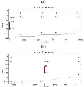
The first step to use the simulator is to define the environmental configuration. As an example the bathymetry of the region north of the Formiche di Grosseto in the west coast of Italy was used together with the source receiver range configuration, as shown in figure 5. The maximum source receiver range was chosen to be 9.5 km in a mildly range dependent transect (source locations A-D stations) and 6.5 km along a moderate range dependent transect (E and F stations). The water depth is approximately 100 m along transect A-D while it varies from 110 to 90 in the downslope case F and from 110 to 130 in the upslope case E.
Figure 5: South Elba bathymethry and source – receiver geometry during the simulation tests.
On each station the source was considered either static or mobile. In the static case the source was located 10 m above the bottom. In the mobile case, the source movement was simulated by a target sliding away from the receiver at an horizontal speed of 1.5 m/s and increasing depth at a rate of 0.05 m/s. Since the data sequences were 20 s duration, the mobile source displacement during transmission was approximately 30 m in the horizontal and 1 m in the vertical which, in general, and at the frequency of 25 kHz, causes a significant channel mismatch. Source - receiver transmit geometry along the two transects of figure 5 are shown in figure 6 for the mildly range dependent along track A-D (a) and the moderate range dependent tracks E-F (b). The receiving array is shown in both plots having 16 hydrophones at 2 m spacing located between 50 and 80 m depth, while the short lines on each station represent the source movement during transmissions (not to scale).
From the environmental point view the water column was characterized by the sound speed profile and the generic bottom properties of [8]. The sound velocity profile (see figure 7) is characteristic of the summer period in that area with a thin thermocline and a strongly downward refracting profile extending to 40 m depth. The sediment is formed by a thick mud layer to the north and northeast of the receiving array location (transect A-D and station F) with a compressional speed of 1465 m/s, a density of 1.5 g/cm3 and a compressional attenuation of 0.06 dB/λ. To the south and southeast (location E) the bottom is characterized by a fine-mud sand layer with 1537 m/s compressional speed, a density of 1.8 g/cm3 and a compressional attenuation of 0.1 dB/λ.
5.1 Transmitted and received signals
The channel frequency response was computer modeled for different transducer-array ranges, for different transducer depths (also different for mobile and fixed nodes) along various propagation transects including upslope,
(a)
(b)
Figure 6: Sketch of the source receiver transects: along the mildly range dependent track A-D (a) and along the
moderate range dependent track E - F (b). The 16-hydrophone vertical array is located between 50 and 80 m
depth at zero km range on each case. Short lines on each location represent source movement during transmissions
(not to scale)
Figure 7: Sound Speed Profile
downslope and mildly ranges dependent propagation scenarios. The bandwidth is within the 4 kHz around a center frequency of 25.6 kHz. Ray trace model TRACE [8] was selected for the channel frequency response modeling and to account for range dependent water column and bottom properties. The receiving array has 16 hydrophone 2 m spaced with the first hydrophone placed at 50m depth and is placed nearby the Formiche di Grosseto as it can be seen in figure 5.
BPSK signals with 2000 bits/sec and a root-raised cosine 50% roll-off pulse-shape were used as transmitted signals for all simulations. Those 3kHz signals were filtered considering the channel time variability, and after being received by the 16 hydrophones array and after noise addition, were applied to the FSpTR equalizer for
demodulation of the transmitted data sequence. The IR estimate required by the environmental equalizer was considered to be the initial IR given by the acoustic propagation simulator.
To make the simulation more realistic additive white noise with a mean power equal to signal power was considered, resulting in a signal-to-noise ratio (SNR) of zero dB for the signals captured on each hydrophone. It results that for the hydrophones with a lower Transmission Loss (usually those with a shorter source-hydrophone range) a stronger power noise was added. Since the SNR was kept constant, the equalizer performance at various source ranges can be readily compared in terms of its capability to combat ISI and deconvolve the channel time-variable multipath.
5.2 Performance results
Tables 1 and 2 show the mean Transmission Loss (TL) between the source and the array, the environmental equalizer output mean squared error (MSE) and the data error rate (ER) for the cases when the source is stationary and when the source is moving for the geometries and transects described in section 5. The TL was computed as the mean over the hydrophone array of the ratio between the input and the output signals of the channel simulator. The MSE was computed as the mean squared ratio between the transmitted and environmental equalizer demodulated data symbols. The ER was computed as the percentage of symbol errors attained at the environmental equalizer output.
In both tables it can be observed the tendency of the TL to increase with range (at least in transect A-D) with, however, an MSE performance that does not vary linearly with range. In fact, with and without source movement the best performance for communications is attained at location C, at 4.5 km range, rather than at location D at 1.5km range. Strangely enough, location F (6.5 km) presents a performance quite similar to that obtained at location D at 1.5 km range. For location E, when the source is moving, very poor results are attained. When the source is static (sound source near the bottom) the results in station E are quite similar to cases of stations F and B when the source is also placed at 6.5 km range.
Case Range(km) A 9.5 B 6.5 C 4.5 D 1.5 E 6.5 F 6.5 TL(dB) 169.5 153.6 156.4 132.4 131.3 146.5 MSE(dB) -10.1 -13.4 -15.3 -12.6 -13.3 -13.2 ER(%) 0 0 0 0 0 0
Table 1: Source to receiving array transmissions in the static case: transmission loss (TL), environmental equalizer mean square (MSE) and corresponding error rate
(EE) along A - B and E - F tracks
Case Range(km) A 9.5 B 6.5 C 4.5 D 1.5 E 6.5 F 6.5 TL(dB) 158.7 158.6 154.7 135.1 137.0 154.9 MSE(dB) -4.38 -6.51 -8.61 -7.94 -3.13 -7.95 ER(%) 5.3 0.9 0.27 0.34 7.1 0.37
Table 2: Source to receiving array transmissions in the moving case: transmission loss (TL), environmental equalizer mean square (MSE) and corresponding error rate
(EE) along A - B and E - F tracks
Comparing the MSE results obtained in a static environment (table 1) with those attained in a variable environment (table 2) strong performance degradation can be observed. That degradation is due, not only to the 1.5 m/s horizontal movement of the source but specially to the depth change. In fact, it was observed that the environmental equalizer has a stronger capability to compensate for the range mismatch than for the depth mismatch.
(a)
(b)
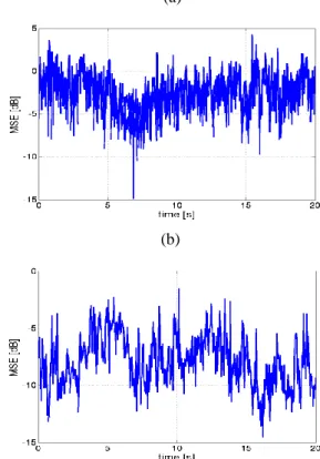
Figure 8: Estimated mean square error during E - F track transmissions at 6.5 km range and with relative source-receiver movement at location: E upslope transmission (a)
and F downslope transmission (b).
Figure 8 shows the simulated MSE performance of the communication system along transects E and F, in the upslope and downslope directions, respectively. It can be seen that there is a quite different behavior of the environmental equalizer for these cases. In fact, location F presents acceptable results, comparable to those of stations B-D. On the other hand, station E, at the same range as F
but to the opposite side of the array, presents an MSE almost always lower by 5 dB than station F. Such fact may be due to the change in bottom properties that was assumed to be, according to the knowledge base of the area of operation, fine sand for E and mud for F. In fact it was observed that in the conditions of station E, the IRs spread up to 70 ms with a strong power in later arrivals that are left uncompensated/unequalized in the present version of the equalizer. Future developments of the environmental equalizer should consider the mitigation of such problem.
6
Conclusion
The objective of developing a time variable acoustic propagation simulator is threefold: (i) to simulate the most appropriate geometric configuration for the network nodes by predicting the locations where the best performance can be attained in given variable and non variable environments; (ii) to study the environmental effects that most degrade a given equalization method and (iii) to allow the comparison of different equalization methods under the same conditions.
In this simulation study only objective (i) was considered. For this objective it can be concluded that location A at a source-array range of 9.5 km is the worst location for the source and that location C at 4.5 km from the array is a better location than location D at 1.5 km. For station E it was observed that it is a good choice to place a fixed node close to the bottom but a very bad one to place a mobile node at mid water depth. This suggests that a performance map can be drawn both for static and dynamic configurations and from that map predict the best distribution for the source locations.
For objective (ii) with the FSpTR equalizer, and despite no detailed description was made in this paper, it was observed that for the actual version of the environmental equalizer the horizontal range movement is the one that is more accurately compensated while a depth variation larger than 2 m is almost left uncompensated. Since the time variable acoustic simulator allows for the observation of the Doppler spread function caused by a given environmental property variability it will be used in future work to improve the robustness of the environmental equalizer to depth variations. A similar study will be carried out for other environmental properties, for example surface agitation and variable sound speed profiles.
Acknowledgements
This work is supported by the Seventh Framework Programme through the UAN project (grant no. 225669). It was also supported by Portuguese Foundation for Science Technology under PHITOM (PTDC/EEA-TEL/71263/ 2006) project.
References
[1] J. C. Preisig, “Performance analysis of adaptive equalization for coherent acoustic communications in the time-varying ocean environment”, J. Acoust. Soc. Am., 118(1):263–278, July 2005.
[2] M. Siderius, M. Porter, P. Hursky, and V. McDonald, “Modeling doppler-sensitive waveforms measured off the coast of Kauai”. In Proc. of Eighth European Conf. on Underwater Acoust., ECUA’06.
[3] Silva, A. and Jesus, S. and Gomes, J. 2007, “Environmental equalizer for underwater
communications”, in Proceedings of the MTS/IEEE Oceans’07, Vancouver, Canada, 2007.
[4] A.J. Silva and S.M. Jesus, “Underwater
Communications Using Virtual Time Reversal in a Variable Geometry Channel”, in Proc. IEEE/MTS Oceans'2002, Biloxi (USA), October.
[5] A. Silva, S. Jesus, and J. Gomes. “Depth and range shift compensation using waveguide invariant
properties”. In Proc. of the UAM’07, Heraklion, Crete, Greece, June 2007.
[6] J. Gomes, A. Silva and S.M. Jesus, “Adaptive spatial combining for passive time-reversed
communications”, Journal of the Acoustical Society of America, 124(2), pp. 1038-1053, August 2008. [7] A. Silva, F. Zabel, C. Martins, S. Ijaz and S.M. Jesus,
“An environmental equalizer for underwater acoustic communications Tested at Hydralab III”, Hydralab III Joint User Meeting, (pdf), Hannover (Germany), February, 2010.
[8] S.M. Jesus, C. Martins and F. Zabel, “Maritime Rapid Environmental Assessment Blue Planet'07: Acoustic Oceanographic Buoys Data Report”, Rep. 03/07, SiPLAB Report, University of Algarve, August 2007.