The Halloween effect in European equity mutual funds

(1)

The Halloween Effect in European Equity Mutual Funds

José Dias Curto

1,*

, Luís Oliveira

1

and Ana Rita Matilde

2

1_{ISCTE-IUL Business School and BRU-UNIDE, Complexo INDEG/ISCTE, Av. Forças Armadas, 1649-026} Lisboa, Portugal

2_{Faculdade de Ciências da Universidade de Lisboa, Campo Grande, 1749-016 Lisboa, Portugal}

Abstract: We extend the evidence on the Halloween effect (returns during the months of May to October tend to be

lower than returns during the months of November to April) in stock markets by examining the return pattern of 145 European Equity Mutual Funds from 1997 to 2013. The main purpose is to investigate if previously predictabilities in equity stock markets returns are reflected in mutual funds. We conclude that (i) the Halloween effect is statistically and economically significant; (ii) this effect has disappeared after the Bouman and Jacobsen (2002) publication; (iii) an investment strategy based on this anomaly clearly beats the buy-and-hold strategy.

JEL Classification code: G10, G14.

Keywords: Halloween effect, market efficiency, calendar anomalies, mutual funds, market returns. 1. INTRODUCTION

The Efficient Market Hypothesis (EMH, hereafter) has over a century of history, being introduced firstly by Bachelier in 1900 and formally presented by Eugene Fama in the 1960s and 1970s. In spite of its widespread acceptance, the efficient markets’ theory was firstly questioned during the 1990s when a few patterns and seasonal effects, also called “anomalies” or “calendar effects”, have been identified in the behaviour of stock prices. The ones commonly tested are the Day-of-the-week effect (especially Monday and Friday; Mazumbder, Chu, Miller & Prather (2008), Tsiakas (2006) and Tong (200)), January effect (Beladi, Chao & Hu (2016b), Lucey & Zhao (2008), Hawawini & Keim (2000) and Canestrelli & Ziemba (2000)), Holiday effect (Hong & Yu (2009)), Christmas effect (Beladi, Chao & Hu (2016a)) and, more recently, the Halloween effect. Even if the EMH does not exclude the possibility of anomalies in the market, and if explored could result in higher profits, the investment strategies based on these patterns cannot be frequent and consistent over time. Therefore, the question remains nowadays, can we trust the stock markets are efficient?

A first important contribution to the “Halloween Effect” (or “Halloween Indicator”) was given by Bouman & Jacobsen (2002) by testing the veracity of the old market wisdom “Sell in May and go away”. Using the monthly stock returns of 37 countries, including developed and emerging markets, from January 1970 to August 1998, they found that average returns for the

*Address correspondence to this author at the ISCTE-IUL Business School and BRU-UNIDE, Complexo INDEG/ISCTE, Av. Forças Armadas, 1649-026 Lisboa, Portugal; E-mail: dias.curto@iscte.pt

period November-April in 36 countries are higher than for the period May-October. Moreover, average returns during the period May-October are not statistically different from zero and are often negative. At the 10 percent significance level, they found statistical evidence of a strong Sell in May effect in 20 stock markets, and particularly strong and statistically significant in European countries. They also showed that this could not be explained by factors such as the January effect, data mining, changes in interest rates and volume and the provision of news. This seasonal pattern questions the EMH mainly because it has been known for quite a time and seems to persist in stock markets.

After the Bouman & Jacobsen (2002) empirical evidence, the investigations directed mainly to three topics. First, which are the reasons for the higher average return in winter and spring time? Second, new empirical evidence was needed against the Halloween effect before and after the Bouman and Jacobsen (2002) paper, insisting on stock markets’ efficiency. Finally, studies to confirm that the effect remains pointing to the conclusion that stock markets are not efficient.

Kamstra, Kramer & Levi (2003) suggest a possible explanation for the Halloween effect. They have documented a similar pattern in stock returns and explain it as a seasonal affective disorder (SAD) effect in stock returns.1 They believe that the decreasing hours of daylight during fall makes investors

1_{SAD is a medical condition whereby the shortness of days leads to}

(2)

depressed, leading to higher risk aversion. Stock returns are lower during the fall and then become relatively higher during the winter months, when days start getting longer (after the winter solstice). Based on stock market index data from countries at various latitudes and both sides of the Equator, the authors found strong evidence that supports the existence of an important effect of SAD on stock market returns around the world. Some authors believe that Kamstra et al. (2003) arguments are not consistent. If they think that the seasonal effect is related to the length of the day, then we expect returns during the spring and summer months, when days are longer, to be higher rather than in winter months.

There are other authors who also suggest that the SAD explanation for the Halloween effect is not reliable. Jacobsen & Marquering (2008) confirmed that there was a strong seasonal effect on stock markets returns for several countries, where returns tend to be lower in summer than in winter time. They mentioned that the correlation between weather and stock returns would be just data-driven and therefore not a potential explanation for the anomaly. Additionally, they also suggested that the SAD argument is not a strong one for countries near the Equator. Kelly & Meschke (2010), based on a more psychological approach, mentioned that the SAD hypothesis is not supported by the psychological literature, as the seasonal patterns for the SAD presented by Kamstra et al. (2003) do not match the general patterns found in depression.

The effect was also studied by Doeswijk (2008) but on a global perspective, with stock markets returns being measured by the MSCI World index and analysed for the 1970-2003 period. He found that returns from May through September tend to be negative or close to zero and those differences in average returns between November-April and May-October periods are about 7.5%, in the 1970-1986 range and 7.7% for 1987-2003. Doeswijk (2008) suggests that the anomaly could result from an optimist cycle, saying that investors think in calendar years, instead of twelve rolling months, and at the beginning of the year they are too optimistic about market growth and earnings. After the summer break, investors become more pessimistic and during the last quarter of the year, they start looking forward to the next calendar year.

In spite of the reasons, several authors insist on the Halloween non-efficiency anomaly. Jacobsen, Mamun & Visaltanachoti (2005) highlight that the Halloween

effect is a market-wide phenomenon, as they found it is not related to the January effect, either to portfolio value, earning price ratios and cash flow price ratios. Bohl and Salm (2010) also investigated the predictive power of stock market returns in January for the subsequent 11 months’ returns across 19 countries. As only 2 out of 19 countries’ stock markets exhibit a robust January effect they conclude that the January effect is not an international phenomenon.

Moskalenko & Reichling (2008) analysed whether a summer break was detected in the Russian stock market. They analyzed the RTS index from 1995 to 2006 and concluded that the September-to-May strategy seemed to perform best amongst stock investments with a duration of eight months, identifying the best month to exit the market as May, supporting the “Sell in May and go away” theory, and that the best entry time was September. Moreover, they saw that the advantage of this strategy is primarily due to market entry time at the end of September, and secondly because of the exit time in May. In their study on U.S. equity sectors in the period 1926-2006, Jacobsen & Visaltanachoti (2009) found that 48 out of 49 industries perform better during the winter when compared to the summer. The authors define an investment strategy (sector rotating strategy) that consists of investing in production-related sectors during the winter and exposing their portfolio to consumer-related sectors during the summer.

More recently Carrazedo, Curto & Oliveira (2016), Haggard & Witte (2010), Jacobsen & Zhang (2010) also documented the Halloween effect. Haggard & Witte (2010) Jacobsen & Zhang (2010) analyse monthly return seasonality using 300 years of UK stock market data (1693-2009) and conclude that the Halloween effect is robust over different subsample periods. They examined whether summer returns are consistently lower than the risk-free rate and came up with a negative summer risk premium for 201 of the 317 years in their sample. Additionally, they also show that trading rules based on the Halloween effect beat the market more than 80% of the time over 5-year horizons. Carrazedo et al. (2016) present economically and statistically empirical evidence that the Halloween effect is significant. Moreover, a trading strategy based on this anomaly works persistently and outperforms the buy-and-hold strategy in 8 out of 10 indices in their sample. The authors suggest that a possible explanation for the Halloween effect may be related to negative average returns during the May–October period, rather than superior performance during the

(3)

November–April period. Urquhart & McGroarty (2014) also found calendar anomalies suggesting that Against the Halloween strategy, are, for example, the findings of Maberly and Pierce (2004), Lucey and Zhao (2008) and Dichlt & Drobetz (2015). Maberly & Pierce (2004) concluded that the anomaly identified in the U.S. equity returns (from April 1982 through April 2003) is due to the presence of two outliers in their sample: “the large monthly declines for October 1987 and August 1998 associated with the stock market crash and collapse of the hedge fund Long-Term Capital Management, respectively” (Maberly and Pierce, 2004 p. 43). Furthermore, they found that the effect disappears after data adjustment. Lucey and Zhao (2008) concluded that the Halloween effect presented by Bouman and Jacobsen (2002) might not exist, being no more than a reflection of the January effect. Contrary to Bouman and Jacobsen’s (2002) results, they saw that the Halloween strategy is not demonstrably more profitable than the buy-and-hold strategy. More recently, Dichlt & Drobetz (2015) found that the Halloween effect strongly weakened or even disappeared in recent years. They argue that their results are robust across different markets and against various parameter variations. Overall, their findings support the theory of efficient capital markets.

Therefore, and based on this brief literature review, we can conclude that there is no consensus regarding the existence of such anomaly, nor about the causes of this effect, if it exists. The million-dollar question remains: Can an investor get higher profits without taking higher risks?

This paper adds to the existing literature by testing the existence of the Halloween effect in the European Equity Mutual Funds industry based on a sample of 145 funds and data from 1997 to 2013. Its contribution to the Halloween effects literature is threefold. First, it focuses on European Equity Mutual Funds. As far as

we know, the Halloween effect has not yet been studied on European euro currency denominated Equity Mutual Funds. Second, we show that the January effect does not explain this anomaly. Finally, we document that the Halloween effect became statistically insignificant, but stills economically significant, after Bouman and Jacobsen’s (2002) publication.

This paper proceeds as follows. Section 2 describes the data, the methodology used and reports the empirical results. Section 3 tests their robustness and documents the existence of the Halloween effect. Finally, Section 4 summarises our concluding remarks.

2. DATA, METHODOLOGY AND EMPIRICAL RESULTS

In this section, we present data that supports our empirical study, and we discuss the methodology used to test the Halloween effect. The main empirical results are also reported in this section.

2.1. Data

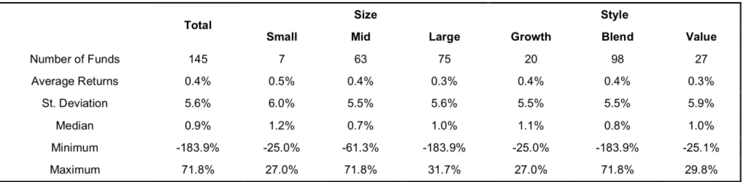
In the empirical analysis, we select 145 funds that invest in equities through European countries and that manage a minimum of 500 million Euros in assets. The main reason for considering European funds is that seasonal effects (especially the Halloween effect) are little known in Europe when compared to American countries, and there are only a few studies about European stock market funds. For example, Andreu, Ortiz and Sarto (2013) examine the seasonal patterns of 69 individual pension plans monthly returns commercialised in Spain and investing in Eurozone equities from 2001 to 2009. Consistent with existing literature, results indicate that a set of portfolios obtain levels of performance during certain months, especially December, that are significantly different from the rest. Table 1: Reports the descriptive statistics based on monthly returns of the funds: average, standard deviation,

median, minimum and maximum returns. Statistical information is reported for small, mid and large-cap funds and growth, blend and value strategy funds.

Size Style

Total

Small Mid Large Growth Blend Value

Number of Funds 145 7 63 75 20 98 27 Average Returns 0.4% 0.5% 0.4% 0.3% 0.4% 0.4% 0.3% St. Deviation 5.6% 6.0% 5.5% 5.6% 5.5% 5.5% 5.9% Median 0.9% 1.2% 0.7% 1.0% 1.1% 0.8% 1.0% Minimum -183.9% -25.0% -61.3% -183.9% -25.0% -183.9% -25.1% Maximum 71.8% 27.0% 71.8% 31.7% 27.0% 71.8% 29.8%

(4)

To study the Halloween effect in European Equities Mutual Funds, we start with monthly price returns over the period 1997-2013. We construct a dataset of monthly returns on 145 mutual funds using Net Asset Value (NAV) data collected from Bloomberg. Table 1 shows the descriptive statistics, based on monthly logarithmic returns of the fund’s NAV for the total and segmented by investment strategy characteristics, size and style.

From the analysis of our sample, we observe that differences between summer and winter average returns are in general large. In most funds, returns over the summer tend to be negative or close to zero, as Figure 1 suggests.

2.2. Funds Average Return

To guarantee that the better performance of winter months is not related to a riskier period, we have also analysed the standard deviation, which, as Figure 2 shows (based on dispersion above and down the X-axis), is similar for both periods for the majority of the analysed funds.

2.3. Average Returns and Risk

This figure reports the average returns and the standard deviation for each of the 145 funds investing in European equities over the period 1997-2013 during the summer (May-October) and during the winter (November-April).

Figure 1: reports the average returns for each of the 145 funds investing in European equities over the period 1997-2013 during

the summer (May-October) and during the winter (November-April).

Figure 2: Reports the average returns for each fund, in the vertical axis, and the standard deviation, in the horizontal axis,

(5)

2.4. Methodology

Fund performance in this study was measured through monthly logarithmic returns defined as;

Rt = ln Pt Pt!1 " #$ % &' (1)

where Pt is the fund’s Net Asset Value (NAV) on the last trading day of the month t and Pt-1 is the fund’s

NAV on the last trading day of the previous month. To test the existence of Halloween effect, and to be consistent with the Bouman and Jacobsen (2002) approach, we use the following simple linear regression equation:

R_t =! + "D_H+#_t (2)

where D_H is a dummy variable, ! and ! are parameters, is the continuously compounded return and !t is the usual error term

2 _!

t = Rt" Et"1

( )

Rt , and

!t! N 0,"

( )

32 .

The variable DH is the Halloween dummy that equals 1 if the month t falls in the period November through April and takes the value 0 in the period May through October. Thus, the constant ! represents the average return for the May-Octoberperiod, when the variable DH takes the value 0, and the coefficient estimate ! represents the difference between the average returns for the two periods November-April and May-October. If a Halloween effect is present, we expect the estimate for the coefficient ! to be statistically different from zero. To estimate the parameters ! and !, we use the Ordinary Least Squares method (OLS).

2.5. Results

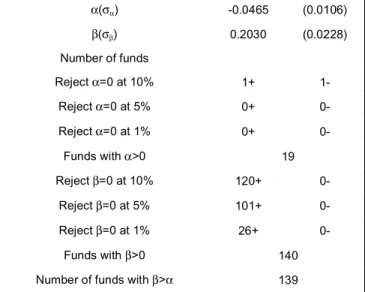
Table 2 reports the results for the annualised average returns, annualised standard errors and general conclusions from the seasonality test specified by the regression in Equation (2).

There is a statistically significant Halloween effect on 120 of the 145 funds in our sample, at the 10

2

In order to deal with errors of non-sphericity we apply the OLS coefficients standard error corrections. White (1980) procedures are applied in cases of heteroscedasticity and Newey and West (1987) procedures in cases of both heteroscedasticity and autocorrelation or only autocorrelation.

percent significance level, and in 101 funds at the 5 percent level. Moreover, we have also seen that, in 139 funds, the return during winter is greater than that in summer, and only at the 10 percent level is it possible to identify a fund with a positive and significant summer average return.

As presented in Subsection 2.1, returns tend to be below average (and negative) in all summer months, especially in August and September, while winter month returns tend to be positive and higher.

Table 2: Shows the average and the standard deviation (between parenthesis) of the estimated

parameters α and β, for the linear regression

presented in Equation 2 (first 2 rows), these figures are annualized; The number of funds to which each null hypothesis was rejected for the 1, 5 and 10 percent significance levels is split by number of funds with a positive sign (+) and number of funds with a negative sign

(–) for the estimates of the parameters α and β3

α(σα)  -0.0465 (0.0106) β(σβ)  0.2030 (0.0228) Number of funds Reject α=0 at 10% 1+ 1- Reject α=0 at 5% 0+ 0- Reject α=0 at 1% 0+ 0- Funds with α>0 19 Reject β=0 at 10% 120+ 0- Reject β=0 at 5% 101+ 0- Reject β=0 at 1% 26+ 0- Funds with β>0 140

Number of funds with β>α 139

2.6. Halloween Effect Statistical Significance

We have just tested whether average returns during the winter are higher than during the summer. A discussion point worth analysing is whether the difference between these periods is due to the performance of specific months rather than that of the whole period.

3

In Table 2 the interior grid line that separates the numbers should be removed.

(6)

The January effect is an anomaly of stock prices behaviour identified as a positive abnormal return between 31st December and the end of the first week of January. For that reason, higher returns during winter months could merely be due to the January effect. To discard that possibility, we test whether the Halloween effect is in fact due to the January effect. To do so, we run Equation (3) which considers an additional dummy variable.

Rt=! + "1Dadj+"2Dadj+#t (3)

Where, Djan, is the additional dummy variable which takes the value 1 in January and 0 otherwise to control the Halloween effect for the well-known January effect. The dummy variable for the Halloween effect, denoted

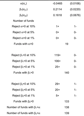
by Dadj, is now adjusted, so that it takes the value 1 in the November to Aprilperiod, except in January, and 0 in May to October. Table 3 summarizes the results.

2.7. Halloween Effect Statistical Significance Controlled for the January Effect

We found that the Halloween effect is still present in most of the funds: 119 of the 120 funds where we previously found a significant Halloween effect (Table 2). The January effect is only statistically significant and positive for 29 funds.

Therefore, we reject the hypothesis that the Halloween effect is due to the January effect. Moreover, we can say that, for most funds, the January effect is not present in our sample although, from our analysis in Subsection 2.3, we saw that returns seem to vary in different months, thus demonstrating the need to test whether this difference is statistically significant.

The parametric F test examines the joint significance of the estimates for all the twelve months via the following equation:

R_t =!₁+!₂D_2t+!₃D_3t+ ...+ !₁₂D_12t+"_t (4) As defined before, R_t is the continuously compounded return, and !t = Rt" Et"1

( )

Rt . Each Dit is

a dummy variable that takes the value 1 for month i and 0 otherwise, !1 is the average return for January and !i is the coefficient for month i, which represents

the difference between January returns and returns in other months. If returns for each month are similar we expect that !i, where i goes from 2 to 12, are jointly

insignificant, which means that in the global model significance test, we will not reject the null hypothesis which consists:

H0:!2=!3= ... =!11=!12= 0

In line with what Jacobsen and Zhang (2010) reported in their results, our analysis indicates that there are statistically significant differences between months for some funds. However, this test does not clarify which months contribute for this seasonality. To do so, we will estimate the following regression for each month:

Rt =! + "Dit+#t (5)

where Di is the dummy variable that takes the value 1

if t falls in the month i, and takes the value 0 otherwise. Table 3: This table shows the average of the estimated

parameters ! , !1 and !2 as well as the

average standard error (between parenthesis) for the regression presented in Equation 3

(first three rows), both statistics are

annualized; The number of funds to which each null hypothesis was rejected for the 1, 5 and 10 percent levels is split by number of funds with a positive sign (+) and number of funds with a negative sign (-) for the estimates

of the parameters ! , !1 and !2

α(σα)  -0.0465 (0.0106) β1(σβ1)  0.2114 (0.0220) β2(σβ2)  0.1618 (0.0676) Number of funds Reject α=0 at 10% 1+ 1- Reject α=0 at 5% 0+ 0- Reject α=0 at 1% 0+ 0- Funds with α>0 19 Reject β1=0 at 10% 119+ 0- Reject β1=0 at 5% 106+ 0- Reject β1=0 at 1% 25+ 0- Funds with β1>0 140 Reject β2=0 at 10% 29+ 1- Reject β2=0 at 5% 20+ 1- Reject β2=0 at 1% 5+ 1- Funds with β2>0 133

Number of funds with β1>α 138

(7)

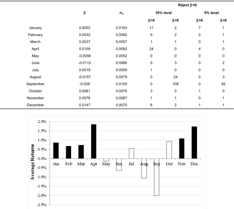
The coefficient α represents the expected return for months other than i and β is the accrual average return for month i when compared with the average return of the other months. The results are presented in Table 4.

2.8. Differences in Monthly Average Returns

Table 4 demonstrates that September returns are responsible for bad performance in average returns for 108 funds, at the 10 percent level, and for 82 funds if we require a 5 percent level. Effectively, the lowest monthly average return is September; however, we

were also expecting April to be a positively significant month, regarding average returns, which happens but only for 24 funds at the 10 percent level and that number falls to 4 if we require a 5 percent level. From the observation of Figure 3, the average returns during the winter are positive for each of the months in that period. Contrary to our expectations, returns are not unusually high in January but are in December and April, while returns during summer months are lower and particularly bad in August and September.

Table 4: Shows the average of the estimated parameter β, as well as the average standard error (columns 2 and 3) for

each month. Columns 4 to 7 present the number of funds to which we reject the null hypothesis that β is 0 at

the 10% and 5% significance levels split by the respective sign

      Reject β=0   β  σβ  10% level 5% level       β>0 β<0 β>0 β<0 January 0.0052 0.0193 11 2 7 1 February 0.0032 0.0082 0 2 0 1 March 0.0037 0.0057 1 1 0 1 April 0.0159 0.0082 24 0 4 0 May -0.0056 0.0052 0 0 0 0 June -0.0112 0.0066 0 3 0 2 July 0.0019 0.0059 1 0 0 0 August -0.0157 0.0079 0 24 0 3 September -0.026 0.0105 0 108 0 82 October 0.0061 0.0076 3 0 1 0 November 0.0076 0.0087 1 1 0 1 December 0.0147 0.0075 6 2 1 1

Figure 3: Reports the average returns for each month. Black columns are related to months in the Summer and white columns

(8)

2.9. Average Returns by Month

Figure 3 reports the annualised average returns for each month. Black columns are related to winter months and white columns are related to summer months.

3. ROBUSTNESS CHECKS

In this section, we will test if the Halloween effect is correctly identified. For that purpose, we will first analyse whether the Halloween effect is found in funds with different sizes and investment strategies. We will then test whether the anomaly is still significant when we use daily returns instead of monthly figures. Hereafter, we study if the Halloween effect is no more than a good performance during the last quarter of the year, October through December, or if it is due to a poor performance in the third quarter, July through September.

It is important to test whether the anomaly is still present in the European Mutual Funds industry after the Bouman and Jacobsen publication in 2002. Otherwise, conclusions from this study could be wrongly assigned to the period from 1997 through 2013, if the effect disappeared after 2002. The results appear in Subsection 3.4.

Finally, in Subsection 3.5 we compare the performance of two investment strategies, one based on the “buy-and-hold” and the other based on the Halloween strategy, which is no more than investing in European Mutual Funds during the winter and investing in a risk-free asset during the summer.

3.1. Size and Style Effects

The first point to check is if the Halloween effect is present in all type of funds, regardless of fund size or investment style. We then split the funds in our sample by investments in companies’ size: small, mid or large cap; or by investment style: value, blend or growth. To better establish the distinction, we exclude the mid and the blend funds from this analysis. The results, obtained from the regression in Equation (2) are summarised in Table 5 and Table 6.

3.2. Halloween Effect and Size Investment Effect

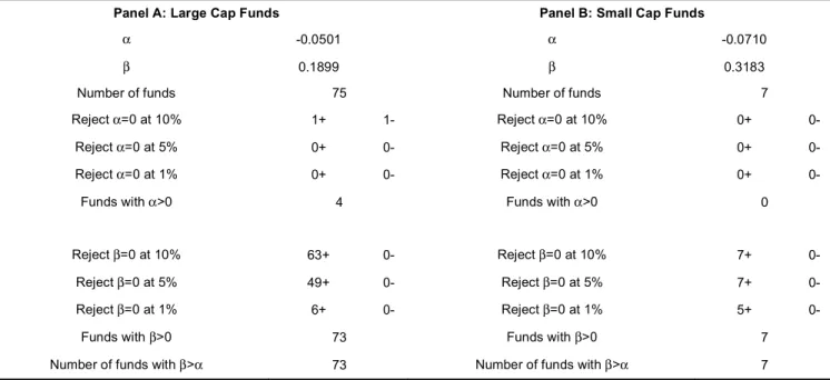
Table 5, Panel A and Panel B, shows the results for large and small cap funds, respectively. The Halloween effect appears to be present in all the small-cap funds at 10 and 5 percent significance level, while it remains present in 5 of the 7 funds at the 1 percent significance level. For large cap funds, the Halloween effect is present in 49 of the 75 large cap funds at the 5 percent significance level. It is important to notice that returns Table 5: This table is divided into two panels. Panel A shows the Halloween effect tested for the large-cap funds, and Panel B shows the Halloween effect tested for the small cap funds. The first two rows in each panel present

the average of the estimates for the parameters α and β, both figures are annualized. The number of funds to

which each null hypothesis was rejected for the 1, 5 and 10 percent levels is splited by the number of funds with a positive sign (+) and number of funds with a negative sign (-) for the estimates of the parameters α and β

Panel A: Large Cap Funds Panel B: Small Cap Funds

α -0.0501 α -0.0710

β 0.1899 β 0.3183

Number of funds 75 Number of funds 7

Reject α=0 at 10% 1+ 1- Reject α=0 at 10% 0+ 0-

Funds with α>0 4 Funds with α>0 0

Reject β=0 at 10% 63+ 0- Reject β=0 at 10% 7+ 0-

Funds with β>0 73 Funds with β>0 7

(9)

for 73 large cap funds are higher during the winter than during the summer and that returns during the summer are only positive (but not statistically significant at least at the 10 percent significance level) for 4 funds.

3.3. Halloween Effect and the Style Investment Effect

Table 6, Shows a similar summary of the analysis but this time for the value and growth strategy funds. Panel A reports the results for value style funds, and Panel B reports the results for growth style funds. For both investment styles, all the returns are higher during the winter than during the summer. Moreover, summer

returns are positive (even though not statistically significant) for only one fund in each group. The Halloween anomaly is present in all the growth strategy funds at the 10 percent level and remains present in 90% of the growth funds at the 5 percent level.

From this analysis, we conclude that the Halloween effect appears to be equally present in small cap and large cap funds and value style and growth style funds, although it is important to state that, due to the small number of funds in each group, we cannot generalise these conclusions.

Table 6: This table is divided into two panels. Panel A shows the Halloween effect tested for the value style funds, and Panel B shows the Halloween effect tested for the growth style funds. The first two rows in each panel

present the average of the estimates of the parameters α and β, both figures are annualized. The number of

funds to which each null hypothesis was rejected for the 1, 5 and 10 percent levels is split by the number of funds with a positive sign (+) and number of funds with a negative sign (-) for the estimates of the

parameters α and β

Panel A: Value Style Funds Panel B: Growth Style Funds

α -0.0530 α -0.0598

β 0.2073 β 0.2524

Number of funds 27 Number of funds 20

Funds with α>0 1 Funds with α>0 1

Funds with β>0 27 Funds with β>0 20

Number of funds with β>α 27 Number of funds with β>α 7

Table 7: Shows the average of the estimated parameters α and β of the regression Equation 2 (rows 1 and 2) using

daily returns, figures are annualized; The number of funds to which each null hypothesis was rejected for the 1, 5 and 10 percent levels is split in number of funds with a positive sign (+) and number of funds with a

negative sign (-) for the estimates of the parameters α and β. The results for monthly returns were presented

in Table 2 and are repeated here for comparisons

  Daily Returns Monthly Returns

α -0.0022 -0.0465 β 0.0086 0.2030 Number of funds Reject α=0 at 10% 2+ 4- 1+ 1- Reject α=0 at 5% 1+ 0- 0+ 0- Reject α=0 at 1% 0+ 0- 0+ 0- Reject β=0 at 10% 106+ 0- 120+ 0- Reject β=0 at 5% 61+ 0- 101+ 0- Reject β=0 at 1% 26+ 0- 26+ 0-

(10)

3.4. Daily Frequency

Another important issue to investigate is whether we still find a statistically significant Halloween effect if the data frequency of the observations is reduced, i.e. if we use daily prices instead of monthly prices. In the current section, we repeat the test for the presence of the Halloween effect using regression Equation (2).

Results for daily prices are slightly different from those presented in Table 2. In Table 7, the average estimates of α and β are now closer to 0, but we still have a negative value for the average α and a positive value for the average β. As for the Halloween effect, we see that it is now statistically significant at the 10 percent level for 106 funds, 14 funds fewer than before, although at the 5 percent level we “lose” 40 funds with the change on data frequency.

3.5. Halloween Effect Statistical Significance Using Daily Observations

Table 7, Shows the average of the estimated parameters α and β of the regression Equation 2 (rows 1 and 2) using daily returns, figures are annualized; The number of funds to which each null hypothesis was rejected for the 1, 5 and 10 percent levels is split in number of funds with a positive sign (+) and number of funds with a negative sign (-) for the estimates of the parameters α and β. The results for monthly returns were presented in Table 2 and are repeated here for comparisons.

3.6. Recovery of the Performance

Doeswijk (2009) argues that funds managers try to beat the benchmark in the winter months, in order to close the year with better results. The monthly analysis, in Subsection 2.3, indicates that returns are generally high in last quarter of the year. An interesting analysis would be to check whether these three months are indeed responsible for the winter performance. To test this, we will follow the usual approach and consider a new equation similar to the one of Equation (2):

Rt=! + "DQ4+#t (6)

As usual, Rt is the continuously compounded

return and !t= Rt" Et"1

( )

Rt . DQ4 is the dummy variable

that takes the value 1 for October, November and December and 0 otherwise, β is the coefficient estimate that represents the difference between the average returns and the returns in the fourth quarter. Table 8 provides the results.

3.7. Influence of the Fourth Quarter in the Overall Performance

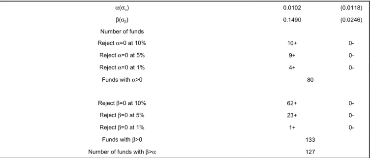
From the results reported in Table 8, we can see that the fourth quarter performance is statistically significant and positive for about 42% of the funds at the 10 percent significance level. However, that value falls to only 17% if we consider a 5 percent level. It seems unreliable that the fourth quarter performance is responsible for the higher winter returns.

Table 8: Shows the average of the estimated parameters α and β, as well as the average standard error for the

regression in Equation 6 (first two rows), figures are annualized; The number of funds to which each null hypothesis was rejected for the 1, 5 and 10 percent levels is split by number of funds with a positive sign (+)

and number of funds with a negative sign (-) for the estimates of the parameters α and β

α(σα)  0.0102 (0.0118) β(σβ)  0.1490 (0.0246) Number of funds Reject α=0 at 10% 10+ 0- Reject α=0 at 5% 9+ 0- Reject α=0 at 1% 4+ 0- Funds with α>0 80 Reject β=0 at 10% 62+ 0- Reject β=0 at 5% 23+ 0- Reject β=0 at 1% 1+ 0- Funds with β>0 133

(11)

Based on the analysis of the fourth quarter performance, we can also test whether lower summer returns are due to the underperformance in the third quarter. We then repeat the previous test for Q3 instead of Q4. The results are reported in Table 9. Table 9: Looks only for the third quarter performance in

the overall performance and shows the average of the estimated parameters α and β, as well as the average standard deviation for the regression in Equation 6 (rows 1-2), figures are annualized; The number of funds to which each null hypothesis was rejected for the 1, 5 and 10 percent levels is split by number of funds with a positive sign(+) and number of funds with a negative sign(–) for the estimates of the parameters α and β

α(σα)  0.0979 (0.0111) β(σβ)  -0.1767 (0.0253) Number of funds Reject α=0 at 10% 97+ 0- Reject α=0 at 5% 61+ 0- Reject α=0 at 1% 12+ 0- Funds with α>0 143 Reject β=0 at 10% 1+ 114- Reject β=0 at 5% 0+ 88- Reject β=0 at 1% 0+ 9- Funds with β>0 7

Number of funds with β<α 139

3.8. Influence of the Third Quarter in the Overall Performance

We see now that returns in the third quarter are responsible for the poor performance of about 79% of the funds, and returns in Q3 are lower than during the remaining period of the year for about 96% of the funds.

3.9. The Halloween effect after Bouman and Jacobsen (2002) publication

The Halloween effect received a lot of media attention after the publication of Bouman and Jacobsen’s (2002) paper, as it was the first time that such anomaly had been studied in depth. According to Murphy’s Law, after an anomaly is discovered, it should disappear or reverse itself. In order to discover if the anomaly had disappeared or reversed itself after the Bouman and Jacobsen study, we split the total period of our analysis (1997-2013) into the following sub-periods: before the publication of the study in December 2002 (1997-2002); after the publication of the study and before the crisis (2003-2007); after the publication of the study and during the international financial crisis4 (2008-2013). Before moving to the regression analysis, we study the difference between winter and summer returns in those three above mentioned periods. Figure 4 shows the statistical main

4

The onset of the financial crisis is generally accepted to be late July 2007. In July, 2007, the Fed and the Bank of England provided the first large emergency loan to banks, in response to increasing pressures on the interbank market.

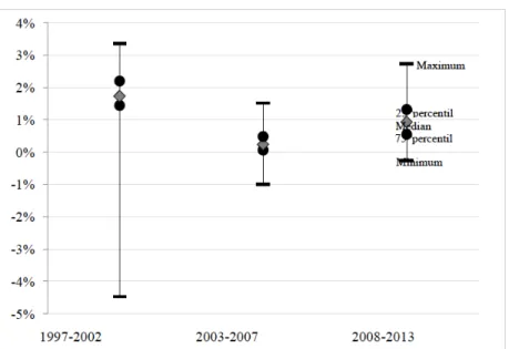
Figure 4: Shows the box plot of the differences between the winter and summer returns for the 145 funds. We present the

minimum, 25th percentile, median, 75th percentile and maximum of the differences for the three periods: 1997-2002, 2003-2007 and 2008-2013.

(12)

characteristics of the differences between the winter and summer returns in each of the above-mentioned periods.

3.10. Differences between the Winter and Summer Returns

In Figure 4, we can see that, in the 1997-2002 period, the 75th percentile was about 2.2%. After the publication of Bouman and Jacobsen’s paper and before the 2008 crisis it falls to 0.5%, while during the crisis it rises to 1.3%.

3.11. Halloween Effect Before and After the Bouman and Jacobsen (2002) Study

While before the Bouman and Jacobsen publication, in 2002, winter returns were slightly different than summer returns, it looks like that, after 2002, those differences disappear, and winter returns are now similar to summer returns.

To check whether our suspicions are correct, we now consider the usual regression defined in Equation (2) for the periods 1997-2002, 2003-2007 and 2008-2013. Table 10 summarises the results. During the 1997-2002 period and at 5 percent significance level,

Table 10: Shows the Average of the Estimated Parameters α and β, for the Regression in Equation 2 (First Two Rows)

for the Period 1997-2002 (Column 2), 2003-2007 (Column 2) and for 2008-2013 (Column 4), Figures are Annualized; The Number of Funds to which each Null Hypothesis was Rejected for the 1, 5 and 10 Percent Levels is Split in Number of Funds with a Positive Sign (+) and Number of Funds with a Negative Sign (-) for

the Estimates of the Parameters α and β

1997-2002 2003-2007 2008-2013 α -0.0076 0.0050 -0.0516 β 0.0189 0.0032 0.0715 Number of funds Reject α=0 at 10% 3+ 32- 25+ 0- 1+ 1- Reject α=0 at 5% 2+ 14- 15+ 0- 1+ 0- Reject α=0 at 1% 2+ 5- 6+ 0- 1+ 0- Reject β=0 at 10% 128+ 0- 10+ 0- 0+ 0- Reject β=0 at 5% 119+ 0- 9+ 0- 0+ 0- Reject β=0 at 1% 47+ 0- 4+ 0- 0+ 0-

Number of funds with β>α 140 27 135

Figure 5: Reports the average returns for each of the 145 funds during the summer (May-October) and the winter

(13)

we found the Halloween effect to be present in 128 funds, although during the 2003-2007 period that anomaly is present in only 10 funds and seems to disappear after 2008. Moreover, in the 1997-2002 period, the estimate for α is statistically significant and negative for 32 funds, at the 10 percent level but that significance disappears after Bouman and Jacobsen’s (2002) publication. These results tell us that summer risk premium might not be negative after the publication and summer returns are now much closer to winter returns, as we have seen before. Therefore, the Halloween effect became statistically insignificant after the publication of Bouman and Jacobsen’s paper, although we cannot say that it is no longer economically significant, as suggested in Figure 5.

3.12. Funds’ Average Return in Summer and Winter Over 2008-2013

Looking at Figure 6 becomes clear that summer average returns are generally positive but lower than winter average returns. If we look in more detail, we will see that monthly returns before and after 2002 are slightly different.

3.13. Average Returns before and after Bouman and Jacobsen’s (2002)

If we can clearly identify the presence of the Halloween effect in the period before the Bouman and Jacobsen publication, after 2002 and before the crisis, average monthly returns are always positive. During the crisis, after July 2007, we see some differences in monthly returns but cannot identify any standard pattern.

3.14.Trading Strategies

It would be interesting to study how a trading strategy based on the Halloween effect would perform in comparison to a simple buy-and-hold strategy. Many economists argue that it is not possible to maximise profits using anomalies like the Halloween effect and that it only exists in the academic world.

For the purpose of studying the strategy based on the Halloween anomaly, we define two investment strategies: the buy-and-hold strategy and the Halloween strategy. For the buy-and-hold strategy, we assume that the investor holds the portfolio for the

Figure 6: Reports the average returns for each month before (1997-2002) and after the Bouman and Jacobsen publication.

Columns in grey are referring to Summer months (May to October) and columns in black are referring to Winter months (November to April).

Table 11: Shows the Percentage of Funds in which the Halloween Strategy Bets the Buy-and-Hold Strategy, for the Return and for the Reward-to-Risk Ratio and Split by Period. For Example, This Table Reports that in the Period 1997-2002, the Halloween Strategy has Out performed the Buy-and-Hold Strategy in 99% of the Funds in Our Sample

Percentage of Funds in which the Halloween Strategy Beats the Buy-and-Hold Strategy

1997-2013 1997-2002 2003-2007 2008-2013 Return 99% 99% 7% 99% Reward-to-Risk ratio 93% 97% 99% 99%

(14)

entire period. For the Halloween strategy, we assume that the investor buys a portfolio at the end of October and sells that portfolio at the end of April, the investor then invests in a risk-free asset from the end of April through the end of October. The risk-free rate used corresponds to the continuously-compounded Interbank Rate: the Libor ECU 6 months, from October 1997 to December 1998, and the Euribor 6 months, from January 1999 to October 20135.

Table 11 reports the percentage of funds where the Halloween strategy beats the buy-and-hold strategy in two characteristics: (i) return, percentage of funds in which the Halloween strategy outperformed the buy-and-hold strategy; (ii) reward-to-risk ratio, percentage of funds in which the reward-to-risk ratio of the Halloween strategy was greater than the reward-to-risk ratio of the buy-and-hold strategy.

3.15. Halloween Strategy Versus Buy-and-Hold Strategy

During the period 1997-2013, the Halloween strategy outperforms the buy-and-hold strategy in about 99% of the funds. This contradicts financial principals stating that investors can get higher returns if, and only if, they take greater risks. During the period 1997-2002, our results are in line with those of Bouman and Jacobsen (2002) who found that the Halloween strategy beats the buy-and-hold strategy for about 90%

5

To save space, the results (annualized returns, standard deviation and reward-to-risk ratio) for both strategies and for each fund are not reported here but are available upon request.

of the countries in their study. Moreover, our results support also those presented by Carrazedo et al. (2016). The authors point out, in their Scenario 2, that in 76% of the indices studied (96% if one considers only the Eurozone indices) the Halloween effect beats the buy-and-hold strategy. Figure 7

3.16. Cumulative Wealth for the Two Investment Strategies

After the analysis of the trading strategies, where we concluded that average monthly returns are always positive over the period 2003-2007, we were not expecting the Halloween strategy to beat the buy-and-hold strategy; this only happens with 7% of the funds. Curiously, during the crisis period, 2007-2013, the percentage of funds that the Halloween strategy beats the buy-and-hold strategy, rises again to 99%.

The Halloween strategy seems to be an alternative way to deal with this market anomaly, at least it was before the Bouman and Jacobsen (2002) publication. According to our analysis, the Halloween strategy beats the buy-and-hold strategy in only 56% of the funds for the entire period after the Bouman and Jacobsen (2002) publication, 2003-2013.

As we show in Subsections 2.3 and 3.3, lower summer returns identified at the beginning of the study are no longer negative after 2002, and in some cases, they are even greater than winter returns. Therefore, it seems obvious that, after 2002, the summer risk premium became positive for most of the funds and the Halloween strategy can no longer beat the buy-and-hold strategy, at least with any degree of certainty. Figure 7: Reports the cumulative wealth for the buy-and-hold strategy (dotted line) and the Halloween strategy (black line),

(15)

While initially, we thought that the Halloween strategy was an opportunity to avoid the lower returns from the Halloween effect, we now demonstrate that it is not clear that this strategy is still an exploitable opportunity after 2002.

4. CONCLUDING REMARKS

The “Sell in May and go away” is an old adage that tells us that returns are greater during the months of November to April (winter) than during May to October (summer) period. This paper studied the so-called Halloween effect market anomaly in European Equity Mutual Funds following the publication of Bouman and Jacobsen’s (2002) paper.

We used monthly logarithmic returns of 145 different sized Equity Mutual Funds that employed different investment strategies in Europe. Data in our sample covered the period from 1997 to 2013.

Our first conclusion is that the Halloween effect was economically significant in 139 of the 145 funds in our sample. Secondly, another important point is that mutual funds returns during the six-month period from May to October are, on average, close to zero or even negative, while winter returns are unusually large. This anomaly goes against the EMH that market returns should not be predictably negative.

Thirdly, we conclude that the Halloween effect is statistically significant at the 10 percent level for 120 of the 145 funds in our sample, which means that there are statistically significant differences between winter and summer average returns and that winter returns are higher than summer returns. It is also important to note that we arrived at similar conclusions when we repeated the regression analysis with daily returns.

Fourthly, we reject the hypothesis that the Halloween effect is explained by the January effect; neither did we find the January effect present in the European Equity Mutual Funds. Another interesting conclusion is that the Halloween effect is not explained by better performance during winter but rather by a poor performance during the third quarter of the year, thus explaining the anomaly. We found this explanation valid for 114 of the 120 funds where the anomaly was identified.

The fifth conclusion came from the analysis of the investment strategies: the first based on the Halloween effect and the second based on the buy-and-hold strategy. Regarding average returns, the Halloween

strategy outperforms the buy-and-hold strategy in 144 funds and, regarding the reward-to-risk, in 135 funds the ratio is higher for the Halloween strategy than for the buy-and-hold strategy. Therefore, the Halloween strategy is an exploitable opportunity.

One important point that we cover in this article is that if the Halloween effect became statistically insignificant after the publication of Bouman and Jacobsen’s (2002) paper, is market efficiency working? Although we would like to say yes, the Halloween effect remained economically significant after the start of the Euro crisis in the second half of 2007, which indicates that it still represents an exploitable opportunity.

Our findings suggest that the Halloween effect is present in European Equity Mutual Funds and a strategy based on this anomaly provides abnormal profits. We also suggest that the negative returns during the summer months, which are primarily during the third quarter, might be one of the explanations for this calendar anomaly; however, further research might be needed.

The EMH has over a century of history; however, no one knows the answer to the question: “Are stock markets efficient?” We have developed the study of the Halloween effect and pointed in different directions that may lead to the puzzle being solved.

REFERENCES

[1] Andreu L, Ortiz C and Sarto J. Seasonal Anomalies in Pension Plans. Journal of Behavioral Finance 2013; 14: 301-310.

https://doi.org/10.1080/15427560.2013.849705

[2] Beladi H, Chao CC and Hu M. The Christmas effect–special dividend announcements. International Review of Financial Analysis 2016a; 43: 15-30.

https://doi.org/10.1016/j.irfa.2015.10.004

[3] Beladi H, Chao CC and Hu M. Another January effect – evidence from stock split announcements. International Review of Financial Analysis 2016b; 44: 123-138.

[4] Bohl M and Salm C. The other January effect: international evidence. The European Journal of Finance 2010; 16: 173-182.

https://doi.org/10.1080/13518470903037953

[5] Bouman S and Jacobsen B. The Halloween Indicator, "Sell in May and Go Away": Another Puzzle. American Economic Review 2002; 92: 1618-1635.

https://doi.org/10.1257/000282802762024683

[6] Canestrelli E and Ziemba W. Seasonal anomalies in the Italian stock market 1973-1993. In D. Keim &W. Ziemba (Eds.). Security market imperfections in world wide equity markets 2000.

[7] Carrazedo T, Curto JD and Oliveira L. The Halloween Effect in European Sectors. Research in International Business and Finance 2016; 37: 489-500.

(16)

[8] Dichtl H and Drobetz W. Sell in May and Go away: Still good advice for investors? International Review of Financial Analysis 2015; 38: 29-43.

[9] Doeswijk R. The Optimism Cycle: Sell in May, The Economist 2008; 156: 175-200.

[10] Fama E. Efficient Capital Markets: A Review of Theory and Empirical Work. The Journal of Finance 2008; 25: 383-417.

https://doi.org/10.2307/2325486

[11] Hagagrd KS and Witte HD. The Halloween effect: trick or treat? International Review of Financial Analysis 2010; 19: 379-387.

[12] Hawawini G and Keim D. The cross section of common stock returns—A review of the evidence and some new findings. In D. Keim & W. Ziemba (Eds.), Security market imperfections in world wide equity markets 2000.

[13] Hong H and Yu J. Gone Fishing: Seasonality in Trading Activity and Asset Prices. Journal of Financial Markets 2009; 12: 672-702.

https://doi.org/10.1016/j.finmar.2009.06.001

[14] Jacobsen B, Mamun A and Visaltanachoti N. Seasonal, Size and Value Anomalies. Working paper, Massey University 2005. Available at SSRN: http://ssrn.com/abstract=784186 or http://dx.doi.org/10.2139/ssrn.784186.

https://doi.org/10.2139/ssrn.784186

[15] Jacobsen B and Marquering W. Is it the weather?. Journal of Banking and Finance 2008; 32: 526-540.

https://doi.org/10.1016/j.jbankfin.2007.08.004

[16] Jacobsen B and Marquering W. Is it the weather? Response. Journal of Banking and Finance 2009; 33: 583-587.

[17] Jacobsen B and Visaltanachoti N. The Halloween effect in US Sectors. The Financial Review 2009; 44: 437-459.

https://doi.org/10.1111/j.1540-6288.2009.00224.x

[18] Kamstra M, Kramer L and Levi M. Winter Blues: A SAD Stock Market Cycle. American Economic Review 2003; 93: 324-343.

https://doi.org/10.1257/000282803321455322

[19] Kelly P and Meschke F. Sentiment and stock returns: The SAD anomaly revisited. Journal of Banking and Finance

2010; 34: 1308-1326.

[20] Lucey B and Zhao S. Halloween or January? Yet Another Puzzle, International Review of Financial Analysis 2008; 17: 1055-1069.

[21] Mayberly E and Pierce R. Stock Market Efficiency Withstands another Challenge: Solving the "Sell in May/Buy after Halloween" Puzzle. Econ Journal Watch 2004; 1: 29-46. [22] Mazumber MI, Chu TH, Miller EM and Prather LJ. International day-of-the-week effects: an empirical examination of iShares. International Review of Financial Analysis 2008; 17: 699-715.

[23] Moskalenko E and Reichling P. Sell in May and Go Away" on the Russian Stock Market, Transformation in der Ökonomie - Festschrift für Gerhard Schwödiauer zum 2008; 65(Chapter IV): 257-267.

[24] Newey W and West K. A simple, positive semi-definite, heteroskedasticity and autocorrelation consistent covariance matrix. Econometrica 1987; 55: 703-708.

https://doi.org/10.2307/1913610

[25] Tsiakas I. Periodic stochastic volatility and fat tails. Journal of Financial Econometrics 2006; 4: 90-135.

https://doi.org/10.1093/jjfinec/nbi023

[26] Tong W. International evidence on weekend anomalies. Journal of Financial Research 2000; 23: 495-522.

https://doi.org/10.1111/j.1475-6803.2000.tb00757.x

[27] Urquhart A and McGroarty F. Calendar effects, market conditions and the Adaptive Market Hypothesis: Evidence from long-run U.S. data. International Review of Financial Analysis 2014; 17: 699-715.

[28] White H. A Heteroscedasticity-Consistent Covariance Matrix Estimator and a Direct Test for Heteroscedasticity. Econometrica 1980; 48: 817-838.

https://doi.org/10.2307/1912934

[29] Zhang C and Jacobsen B. Are Monthly Seasonals Real? A Three Century Perspective. Review of Finance 2013; 17: 1743-1785.