A theoretical Study of H2 Diffusion and adsorption into Carbon Nanotubes using Monte Carlo Simulations

(1)

A Theoretical

Study of H2

Diffusion and

Adsorption into

Carbon Nanotubes

Using MonteCarlo

Simulations

Marco Lerario

Tese de Doutoramento apresentada à

Faculdade de Ciências da Universidade do Porto

A The or et ic al St u d y of H2 Di ffu sio n an d Ad so rp tio n in to Ca rb o n Na n o tu b es Us in g Mo n te C ar lo Si m u la tio n s Ma rc o Le ra rio

Ph

D

FCUP ANO 3.º CICLO

D

(2)

D

A Theoretical Study of

H

₂

Diffusion and

Adsorption into Carbon

Nanotubes Using

MonteCarlo

Simulations

Marco Lerario

Doutoramento em Química

Departamento de Química e Bioquímica 2017

Orientador

(3)

(4)

Acknowledgements

As we all live intertwined, you never know how such small things as a smile, a word, or even just listening, can really make a difference an mean great things for other people. Hence, there are so many I would like to thank, and even more that I should, but I’ll never be able to remember all. Let’s just put in this terms, since we are actually dealing with science and statistics, consider this like a small but representative sample, part of a greater universe, where lots of people, like the ones mentioned here, continuously do their best to support each other and promote others development like their own. I’m certainly grateful to professor Alexandre Magalhães for the patient work done together and the countless challenges we passed through. I’m glad to remember also professor Maria João Ramos for the brilliant conversation where the first ideas of the new algorithm were born.

I thank Elizabeth, Francisca, Kris and Iwona for the gorgeous moments we shared, I’m so grateful for the events that brought us together and I will always feel honoured to be your friend. Henrique, Juliana and Carla, thank you for keeping room 3.26 a warm place to work, meaning that good company matters more than temperature! I thank you Ana for your exceptional support, your kind listening and bright solutions. I would like to thank all my colleagues, in particular Eduardo, Rui and Diana, for your solicitous help and fruitful conversations during all these years.

A special thanks goes to my father and brother, as well as my uncle and aunt and my dearest cousins: even if time and distance divide us, I know you are always at my side (who more lucky than I, and who more supported?). I also thank you Sara, for your kind attention, for your laughs, for your delicious ideas, which offered me some wonderful moments.

I also want to thank Carlos, Luis, Zé Manel, Zé Alberto and all my brothers, for the patience and comprehension as well as your support in the last few months. I cannot forget to thank my “personal trainers” Kika and Virgínia, without your faith and your

(5)

encouragement I would have never gone through all this; in the end, my only fear was that I could disappoint you. Thank you Carla, Francisco, Tiago and Sofia for the precious help that I didn’t even dare to ask; your constant presence made me feel like nothing was impossible! To Margarida, Andreia, Daniela, Zé Pedro, Catarina, and all the friends of the SMC, thank you for your advice, your words, prayers, and specially for the cheerful and refreshing moments we lived in Viseu.

Finally, I thank FCT - Fundação para a Ciência e Tecnologia for the grant SFRH / BD / 90502 / 2012, as well as REQUIMTE - Rede de Química e Tecnologia which offered me the necessary conditions to develop this work.

(6)

Abstract

The interest of this work on Carbon Nano Tubes lies mainly in their shape (cylindrical symmetrical, combined with extreme length) which keeps intertwined opposite char-acteristics like symmetry and randomness. The way they aggregate in real samples, with the formation of bundles, as well as the insurgence of defects creates an extreme variety of pores and different environments which can behave very differently. The affinity for hydrogen, together with its small size, make it the perfect probe molecule for investigating such structures.

The studies found in literature, which are mainly focused on maximising adsorption,

e.g. for automotive application, not always produce reproduccible results or, at least,

their range is extremely wide. This happens not only on the experimental side, but also in theoretical works, thus proving that this subject is very far from being exhausted and that there are still many aspects to be enlightened.

This investigation therefore wants to explore alternative paths, including and combin-ing new effects; the Monte Carlo method offers both the versatility and the capability to adapt to variable environments. We approach the subject of hydrogen interaction in several ways. From a topological point of view we construct potential energy surfaces of the different pores and environments: potential data are gathered from literature and their effect is also object of investigation. Through GC simulations, we found adsorption being very sensitive to such parameters, and explained how the pore size influence the uptake / storage mechanism. The other interesting aspect was accessibility, which has been studied by means of Kinetic Monte Carlo in simulations of diffusion dynamics. Finally, the aim of phase transition studies was to explore the existence of alternative ordered conformations, related to the symmetry of the system. All the code used in this work was written on purpose, with the goal of, in the future, being linked together so that all the aspects can be investigated at once.

(7)

Resumo

O interesse deste trabalho sobre os Nano Tubos de Carbono reside principalmente na sua forma (simétria cilíndrica, combinada com comprimento extremo) que mantém características opostas e entrelaçadas como simetria e aleatoriedade. A forma como se agregam nas amostras reais, com a formação de feixes, bem como a existência de defeitos, cria uma extrema variedade de poros e ambientes diferentes que demonstram comportamentos muito diferentes. A afinidade pelo hidrogénio, juntamente com seu pequeno tamanho, tornam esta molécula uma sonda perfeita para investigar tais estruturas.

Estudos anteriores, destinados principalmente a maximizar a adsorção, e.g. para aplicação na indústria automóvel, nem sempre produzem resultados reprodutíveis ou, pelo menos, a sua dispersão é extremamente elevada. Isto acontece não só em trabalho experimental, mas também em trabalho teórico demonstrando que este assunto está muito longe de ser esgotado e que existe um grande número de aspetos que necessitam ser clarificados.

A presente investigação portanto pretende explorar caminhos alternativos que incluem e combinam novos efeitos. O método Monte Carlo oferece tanto a versatilidade como a capacidade de adaptação a ambientes variáveis. Abordamos o assunto da interação do hidrogénio de várias formas. Do ponto de vista topológico, construímos superfícies de energia potencial dos diferentes poros e ambientes: dados potenciais são coletados da literatura e seu efeito é, também, objeto de investigação. Através de simulações do ensemble grande canónico concluimos que a adsorção é muito sensível a esses parâmetros e explicamos como o tamnho dos poros influencia o mecanismo de captação/armazenamento. O outro aspecto interessante foi a acessibilidade, que tem sido estudada por meio de Monte Carlo Cinético em simulações de dinâmica de difusão. Finalmente, os estudos de transição de fase pretendem explorar a existência de conformações ordenadas alternativas, relacionadas com a simetria do sistema. Todo o código utilizado neste trabalho foi escrito com o objetivo de, no futuro, poder ser interligado para que todos os aspectos possam ser investigados simultaneamente.

(8)

List of Figures

1.1 Wrapping of CNTs. . . . 2

1.2 SWNTs forming bundles. . . . 3

1.3 Emergence of ordered conformations in adsorbed layers. . . 13

2.1 Sampling of a function f(x) with rejection method. . . 21

2.2 Combination of multiple simulations —i (with i = 1, 2, . . .) produces an improved estimation of the DOS (E). . . 43

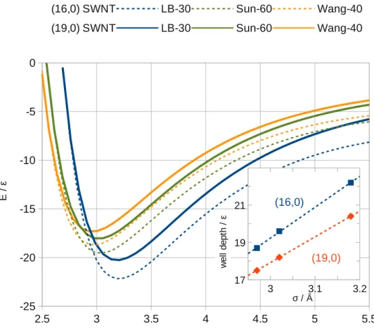
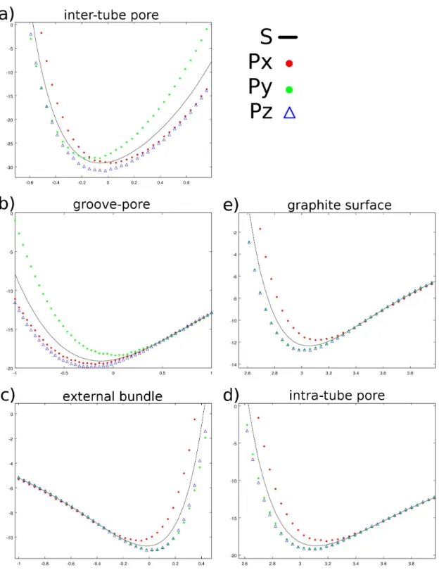
3.1 Inner and outer density around (19,0) SWNT square bundles with dif-ferent spacing. . . 61

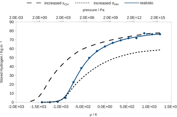
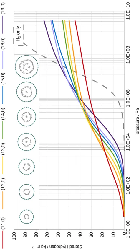
3.2 Shape and energy profiles for different surfaces of a (16, 0) SWNT bundle. 63 3.3 Inside SWNT total energy plot. . . 64

3.4 GCMC simulated adsorption isotherm inside a (16,0) SWNT at 77K. . 66

3.5 Simulated adsorption isotherm of isolated SWNT of different radius at 77K. . . 67

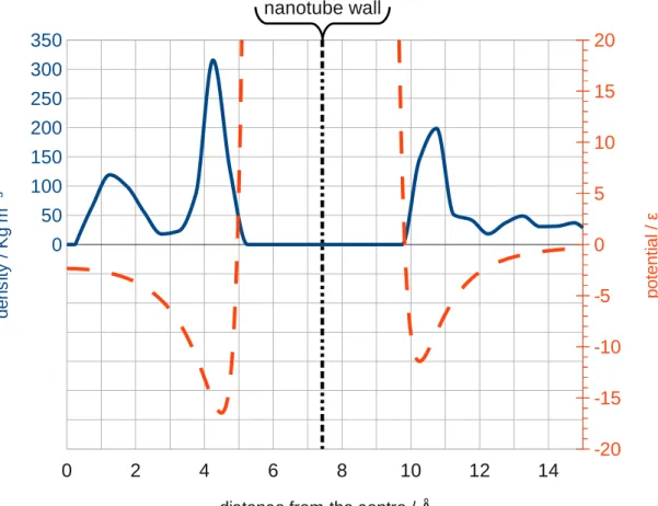
3.6 The simulated H2 radial adsorbed density, at 75K and 62.5atm, inside a (19,0) SWNT and the relative PES radial section. . . 68

3.7 Schematic representation of spherical harmonics. . . 70

3.8 Numerical integration of spherical harmonics interacting with CNT and graphite surface. . . 72

(13)

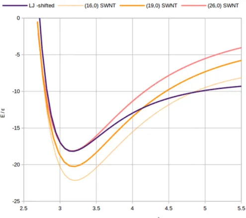
4.1 Comparison between atomistic potentials of (16, 0),(19, 0) and (26, 0)

SWNT with the non-atomistic potential used in simulation (shifted for comparison purposes). . . 80

4.2 Representation of the reference SWNT cell ( R=10Å and L=200Å). . . 83 4.3 Distribution of particles on a projection plane perpendicular to the

lon-gitudinal axis of the SWNT. . . 85

4.4 Fraction of H2-H2 repulsive interactions with distance less than ‡HH in a particular region. . . 86

4.5 Potential Energy Profiles (PEPs) of the simulations with 500, 1000 and 1500 particles. . . 88 4.6 Self-diffusion coefficient as a function of the number of particles used

for simulations where the influence of concentration was studied. . . 90

4.7 Illustration of the difference between the SWNT’s radius and the

effec-tive radius. . . 93

4.8 Distribution of particles on projection plane perpendicular to the

longi-tudinal axis of the SWNT. . . 94

4.9 Radial distribution functions for the simulations performed in order to

study the influence of the SWNT’s length. . . 95

4.10 Distribution of particles on a projection plane perpendicular to the

lon-gitudinal axis of the SWNT. Fixed L = 200Å. . . 96

4.11 Self-diffusion coefficients for the highlighted regions of the SWNTs of

figure 4.10 and the relative particle density. . . 97

4.12 Comparison between the self-diffusion coefficient (Ds) values obtained for the influence of aspect ratio (R/L) and for the influence of the radius. 98

5.1 Ordered-disordered phase diagram for H2 adsorbed on graphite surface from GEMC simulations; snapshots of the two phases are presented in the insets. . . 106

5.2 Stability of the different conformations. . . 107 5.3 TM results of free hydrogen simulations, 1-centre model. . . 108

(14)

5.4 Phase diagram of free hydrogen, 1-centre model. . . 109 5.5 Contour plot of ln [ (µ, ﬂ)] Probability of measuring density ﬂ at

chem-ical potential µ inside a (26,0) CNT at 77K. . . 110

5.6 Contour plot of ln [ (µ, ﬂ)] Probability of measuring density ﬂ at

chem-ical potential µ for free hydrogen at 77K. . . 111

6.1 Evolution of energy and particle number during a GCMC H2 box filling simulation. . . 116

6.2 Splitting between estimations of the relative probability, respectively with

and without conformational rearrangement. . . 118

6.3 Schematic representation of the TMMC algorithm, according to the

im-plementation in MCCCS towhee software. Orange markers are related to the implementation of the new features. . . 119

6.4 The creation of a positive dummy makes the system behave as it had

N + 1 particles. . . 121

(15)

(16)

List of Tables

3.1 Isotropic potentials. . . 59

3.2 Anisotropic interaction potentials. . . 59

3.3 Amount of stored hydrogen (%wt.) inside a (19,0) SWNT at 77K. . . . 65

4.1 Summary of the geometrical parameters, number of particles used of the correspondent zig-zag nanotube and the H2 percentage of mass fraction and diffusion coefficient. . . 84

4.2 Mobility in different zones of the SWNT. . . 92

5.1 Simulation potential parameters. . . 103

6.1 Variables fixed at dummy creation. . . 121

(17)

(18)

List of Abbreviations

ASH Amount of Stored Hydrogen AVB Aggregation Volume Bias BET Brunauer–Emmett–Teller CB Configurational Bias CNF Carbon Nano Fibers CNT Carbon nanotube

CVD Chemical Vapour Deposition

Ds Self-diffusion coefficient

DFT Density Functional Theory DOS Density of States

DWNT Double-walled carbon nanotube FH Feynman Hibbs

GC Grand Canonical

GCMC Grand Canonical Monte Carlo GE Gibbs Ensemble

GEMC Gibbs Ensemble Monte Carlo KMC Kinetic Monte Carlo

LJ Lennard-Jones MC Monte Carlo

MCCCS Monte Carlo for Complex Chemical Systems MD Molecular Dynamics

MWNT Multi-walled Nano Tube PEP Potential Energy Profile PES Potential Energy Surface PI Path Integral

PSD Pore Size Distribution

QENS Quasielastic Neutron Scattering SWNT Single-walled carbon nanotube

(19)

TEM Transmission Electron Microscopy TM Transition Matrix

TMMC Transition Matrix Monte Carlo

(20)

Chapter 1 Introduction

Nanotubes were first synthesized in 1991 and, since then, they have been the focus of multiple studies due to their great potential in many fields [46, 21]. They have unique and specific characteristics, such as their nanometric scale size, hollow and cylindrical shape [41]. These characteristics make them potential materials to be used in catalysis [93], separation and purification processes [49, 11], and also in gas storage and transport[22, 116, 55]. In particular, the storage and transport of fuels like hydrogen and methane - which are renewable energy sources - inside single-walled carbon nanotubes (SWNTs) is of prominent importance because of the increasing necessity to find cleaner alternatives to fossil fuels [37]. In fact, this is a subject of current investigation in the area of automotive applications [21]. There are already some studies about the two main properties that influence the storage and mobility of gases inside SWNTs: their adsorption capacity[16, 39] and the diffusion of gases inside them [9, 73, 72]. However, a consensus has not been established yet about the influence of these parameters on the autonomy and efficiency of those physical processes. Therefore, it is important to understand and clarify the structure-property relationships since it is established that the diffusion depends on the structural pa-rameters of the pores[2].

In this thesis the topic is approached by three points of view: one, strictly quantitative, involve Monte Carlo (MC) simulations of the loading limit capacity of some Carbon Nanotubes (CNTs), different for size and geometry. A more qualitative analysis aims to investigate the accessibility of deeper zones of CNT structures through kinetic Monte Carlo (KMC) simulations. Finally a more specific study focus on hydrogen molecules and their aggregations states, when confined into carbon nano structures.

(21)

1.1 Carbon Nano Tubes

CNTs can be visualized as a single graphene sheet wrapped into a cylindrical tube; according on how many sheets are concentrically wrapped, they can be Single-Walled Nano Tubes (SWNT), Double-Walled Nano Tubes (DWNT) or Multi-Walled Nano Tubes (MWNT).

Moreover, there is not just one way to wrap the sheet, but a virtually infinite variety of CNTs is available.

Figure 1.1: Wrapping of CNTs.

A graphene planar unit cell is defined by two vectors a1 and a2 (see figure 1.1): any

displacement along the plane of a combination of these two vector na1 + ma2 with n, m _{œ N positive integers, generates a point which is indistinguishable from the}

previous one. In order to ideally wrap the plane, it is of course necessary to overlap indistinguishable points, so that the coefficients n and m are sufficient to uniquely identify a wrapping. The only exception is the chiral wrapping, which happens for

m _{”= n ”= 0, because it produces a nanotube not superimposable to its mirror image.}

Therefore any chiral CNT can have two possible orientations. Other ways to wrap generates respectively zig-zag CNTs (m = 0) or armchair (m = n).

From the geometric point of view, since they are made of hexagons wrapped around, CNT section (perpendicular to the wrapping axis T) is more like a polygon than a circle. A common way to define CNT’s size, nevertheless, is to calculate the perimeter of the CNT using the index n and m. Knowing in fact that |a1| = |a2| = lbÔ3, where lb is the bond length of the carbon framework, it is possible to deduce the perimeter.

(22)

Now, assuming that value as it were a circle, it is possible to estimate a radius

R= lbÔ3

2ﬁ Ô

n2+ nm + m2 . (1.1)

Finally, for the sake of completeness, it should be said that the periodicity along the

Z axis varies a lot according to the CNT type. In fact, a zig-zag (n, 0) type CNT is

periodic after just 2n atom, i.e. the next atom in the Z direction is indistinguishable from the first. In the armchair type we have a similar behavior but after 4 distin-guishable atoms. The chiral case instead, is much more complicated. For example, in figure 1.1 (left inset) is represented a chiral wrapping with n = 4 and m = 2: it is clear that the axis T only founds an equivalent atom at 4a1 ≠ 5a2, so the total unit

cell comprises 60 atoms.

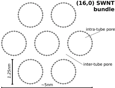
Figure 1.2: SWNTs forming bundles.

Nanotubes tends to aggregate forming bundles in a triangular lattice. Figure 1.2 represents a typical structure which enlighten several different environments. Very hollow pores are situated in the inter-tube spacing. In the case of (16, 0) SWNT bundles, such pores’ size is about 0.2-0.3nm, just enough to host a small hydrogen molecule[94]. On the other hand, according to equation 1.1, their diameter should be 1.25nm, as shown in the picture, so that the available pore size for H2 is about 0.7nm.

The accessibility of these pores in real sample is not obvious, due to the length of CNTs and also to the possibility of their ends being closed by a fullerene-like surface.

(23)

On the outside of the bundle two different surfaces are also identifiable: the convex one around the external CNTs and the groove between two adjacent.

Bundle size can grow up to 20nm as more SWNT are joined together. The extremely high aspect ratio (Length/diameter ≥ 1000) supports the simulation of CNT in periodic limit conditions along their axis (i.e. infinitely long CNTs).

1.2 State of the art

1.2.1 Experimental data

Since their discovery by Iijima et al. [47] CNTs have been investigated as a potential way for hydrogen storage due to their high surface area and the innate inclination of carbon to adsorb gas molecules.

Dillon et al. [22] were the first to publish experimental data on hydrogen adsorption in nano tubes. They developed Temperature programmed Desorption (TPD) techniques in order to exactly measure, by means of a mass spectrometer, the hydrogen amount desorbed by the sample during a heating run. Their sample was firstly heated under vacuum, then exposed to hydrogen at 300 T orr (≥ 40Pa) and finally cooled to 133K. The chamber was then evacuated with concurrent cooling of the sample to 90K. The TPD then consists in plotting the hydrogen mass signal while continuously heating up to 450K. The authors reported a gravimetric storage density of 5-10%wt at room temperature. These values however, are extrapolated from measure of a soot sample containing 0, 1-0, 2% of as-prepared SWNT. Liu C. and Cheng H.-M. in a recent review [61] underlined that, although TPD could possibly have some discrepancies with respect to volumetric or gravimetric analysis because of the small time between the removal of the pressure used for charging the sample and the start of the measures, its advantage is that it detects precisely the presence of hydrogen.

Based on these results, Ye et al. [114] measured hydrogen adsorption on SWNT which they had prepared and purified. To cut the SWNTs and disrupt the rope structure, nanotubes were sonicated for 10h in dimethyl formamide until the sample was completely suspended in the solvent and finally they were extracted by means of vacuum filtration. Volumetric measures, performed with a Sieverts apparatus and after 10h degassing at 220¶C, are reported only for 80K: 8, 2%wt under 12MP a. The

(24)

BET surface ratio (285m2_g≠1 and 1600m2_g≠1 respectively). Transmission Electron

Microscopy (TEM) images show 1, 3nm diameter SWNT packed in triangular lattice bundles of 6-12nm diameter. From these information the authors argue that only external surface is measured by BET method with nitrogen gas. Data show that Saran carbon have higher capacity at pressures below 30bar probably due to the higher accessibility of adsorption sites that saturate rapidly, while SWNT storage increase linearly with increasing pressure. Sonication appeared to increase CNTs’ adsorption by a factor of two at pressures below 60bar. This behaviour has been attributed to the reduction of cohesive energy of the rope structure by means of defect generation. When SWNT aggregates form bundles it is possible to identify 2 different kinds of pores. One is the inner cavity of the CNT (usually not available in as-synthesized CNT which are closed by semi-sphere shaped fullerene molecules), the other is the interstitial pore inter CNT. DWNT and MWNT have also one or more inter-layer pores respectively. Surface of the bundles is also capable of adsorption: the curved external surface and the groove between two adjacent CNTs. Moreover CNT bundles aggregate creating a broad distribution of meso pores. Such diversity, even in adsorption energies, makes difficult to match the measure of the available surface area with the predicted data. Large diameter SWNT (mean value = 1, 85 ± 0, 05nm), synthesized by a semi-continuous hydrogen arc discharge method, were tested for hydrogen adsorption by Liu C. et al. [62]. Their measures consist in monitoring the hydrogen pressure (10-12MP a) in a constant-volume cell containing the sample: the difference between the initial and equilibrium values corresponds to the adsorbed amount. The authors compared as-prepared SWNT adsorption, a sample treated with hydrochloric acid (37%) for 48h and another one that, after having received this HCl treatment, was also heated under vacuum at 773K for 2h. The HCl soak should remove the residual catalysts while the heating should evaporate organic compounds formed on the surface. The latter cause a relevant increase of adsorption: 2%wt, 2, 5%wt and 4, 2%wt are respectively the hydrogen uptake of the three samples which had a purity of 50-60%. It is also reported that almost 80% of hydrogen was adsorbed reversibly, while for desorbing the rest heating at 473K was necessary. However Darkrim et al.[20] argued that two thermal effects should have been taken into account: the gas compression up to the target filling pressure and the gas adsorption during this filling. Both could cause an overestimate of the hydrogen uptake.

It is undoubted that the morphological properties of the adsorbent exert relevant influence on capacity. Still, we can only speculate about their effect. Tarasov et al. [106] carried out sorption measures on SWNT synthesized by the arc discharge method

(25)

using respectively Co and Ni powder or Y Ni2 powder as catalyst. They managed to

purify samples up to 75% and characterised them by TEM. SWNT prepared with Co and Ni powder seemed to be slightly narrower (1, 2nm diameter versus 1, 4nm). The authors reported a 2, 4%wt sorption capacity at 25bar and 77K in conditions of no saturation: application of 35bar nearly doubles such amount. Larger nanotubes have shown 15% higher capacity, it could be nevertheless due to the presence of hydride forming metal, residue of the catalyst. TPD measures have also shown that about 2/3 of the amount is stored in reversible condition and thus desorbed at low temperature while the rest only desorbs at 470¶C as it should be for chemisorbed hydrogen. At room

temperatures, storage capacities dramatically fall: 0, 2-0, 4%wt under 10-30bar of H2

pressure. Besides, at pressure below 25bar, SWNT show even less adsorption capacity than AX21 activated carbon. This trend is then inverted at cryogenic temperature and high pressure: the authors argued it could be due to an increase in inter-tube distance caused by pressure as it was earlier suggested by Ye et al. [114].

Bacsa et al. [3] studied the effect of purification on CNT synthesized by catalytic chemical vapour deposition (CVD). The purification methods they use (oxidative acid treatments or by heating in inert gas) decrease the hydrogen storage. They also argued that decreasing the residual catalyst content does not necessarily lead to an increase in Amount of Stored Hydrogen (ASH) and that increasing the specific surface area does not necessarily increase the hydrogen storage capacity, but other factors are probably involved. One of this could be the volume of the pores whose diameter is shorter than 3nm.

An interesting research published by Shiraishi et al. [94], compares adsorption data at room temperature, respectively from SWNTs and from the so called “peapods” that is

C60 encapsulated SWNTs. The authors mean to study the adsorption mechanism at

room temperature and calculate its potential in CNTs. SWNTs were synthesized by Nd:YAG laser ablation using Ni/Co catalysts. High purification yield was obtained by refluxing samples in aqueous solution of H2O2 for 3h, treating with HCl overnight

and finally ultrasonication in aqueous NaOH (pH = 10-11) for 2h. Then, part of the SWNT was used to synthesize peapods (about 85% filling rate) and finally both samples were heated under vacuum at 973K, 10≠2_{P a} for 1h. Assuming a Langmuir

model and the calculated theoretical adsorption potential of an individual and isolated SWNT being about 0,09eV (1082K) [102], hydrogen adsorption on the outer surface and the intra-tube pores can occur only at low temperature. However comparative TPD results show that hydrogen could adsorb in the interstitial pore of nanotube bundles. SWNT bundles usually aggregate in a triangular lattice, and according to

(26)

this model, authors calculate an interstitial pore diameter of about 0, 2-0, 3nm for the 1, 4nm diameter SWNT used in this experiment. Since calculated intra-CNT pore size is 1nm, they expected adsorption potential in the interstitial to be higher. It has been estimated by means of Kissinger’s plot to be 0, 21eV : a value nevertheless small enough to prove the occurrence of physiorption. They conclude that adsorption capacity at room temperature seems to be enhanced by the presence of small pores of 0, 2-0, 3nm. Adsorption in such small interstitial pores could explain the discrepancy between measured potential and theoretical values.

What can be argued about such kind of small pores is their low accessibility especially in structures with a high aspect ratio as nanotubes usually are. Holt et al. [45] have proved nevertheless that mass transport through CNTs with diameters smaller than 2nm could be faster than predicted by Knudsen model. According to Molecular Dynamics (MD) simulations, they attribute this behaviour to the smoothness of the CNT which cause the emergency of a combined flux resulting from both specular and diffusive collisions, being the Knudsen model purely diffusive and thus slower. Another significant data reported in this work is that hydrocarbons exhibit higher selectivities due to their preferential interaction with the CNT sidewalls. However the authors prepared membranes of straight nanotubes with 2-3µm thickness which result in a smaller aspect ratio than CNTs usually have. Therefore, it is not proven yet that such behavior could occur with free and longer CNTs.

More recently, much effort is being made to understand how adsorption is affected by both morphological (e.g. specific surface area, diameter) and chemical factors (e.g. purification methods). Studies of such kind have also been carried out in the past, but now they seem to explore a wider range of possibilities and not only attempting to maximize adsorption. Raman spectroscopy is often used for characterizing CNTs identified by radial breathing vibrational modes. Information about nanotube diame-ter distribution as well as the ratio between ordered CNT and amorphous carbon are available from spectrum analysis.

Ioannatos and Verykios synthesized SWNTs and MWNTs by CVD and characterized them by Raman spectra, Scanning Electron Microscopy and BET surface (N2 at 77K)

[48]. Adsorption measures were then analysed in terms of hydrogen adsorbed amount on a per unit mass or per unit surface area basis. The latter is very important for comparing MWNT adsorption capacities since not all layers take part in the adsorption process. Since MWNT showed a higher capacity per unit surface area than SWNT, but lower one with respect to the unit mass, the authors argued that nitrogen, used for measuring surface, and hydrogen are not adsorbed in the same way in such

(27)

systems. They also formulate the hypothesis of the existence of specific adsorption sites. This is consistent with the results obtained at 298K since the measured capacity is significantly lower than the calculated value for a complete monolayer adsorption. TPD analysis have nevertheless shown that the adsorption sites on the CNTs surface are relatively uniform and that there are no sites which form very weak or very strong adsorption bonds. At 77K high adsorption capacities exceed the theoretical value for monolayer coverage.

Karatepe and Yuca [50] analysed three ways (HCl, HNO3 , H2SO4; all 3M) of

removing the metal catalysts from the synthesized SWNT and one (30% H2O2 : 3M HCl ) which removes amorphous carbon as well, in order to investigate their possible

effects. ThermoGravimetric analysis and Raman spectroscopy produced information on purity and integrity of nanotubes before and after treatment. For each sample as well as for the as-grown CNTs it was measured adsorption capacity at 77K and pressures up to 100bar. Purification enhanced adsorption and shortened SWNT in all cases. This could be important because it opens the ends, making inner adsorption possible. Although the sample with the highest purity was the one treated by HNO3,

the best storage performance (4.86%wt) has been achieved after purification with

H2O2 : HCl, probably due to the removal of amorphous carbon.

1.2.2 Theoretical studies

Many efforts have been made in theoretical investigation to achieve the maximum storage capacity of SWNT. MC simulations according to the Grand Canonical (GC) ensemble have been widely used to reproduce experimental results and explain storage capacities of various carbon based structures (e.g. SWNTs, MWNTs, CNFs). In fact, GCMC simulation technique, since it is able to generate and remove molecules from the system until reaching equilibrium at a fixed chemical potential, is very suitable for adsorption studies. It can be imagined as a constant temperature and pressure system in equilibrium with an ideal infinite thermal bath which has fixed chemical potential. After Chambers et al. [12] reported spectacular experimental hydrogen storage of 67%wt into CNFs this kind of studies spread very quickly. Rzepka et al. [91] investi-gated by GCMC simulations the storage capacities of carbon slit pores (constituted by two graphitic layers separated by a certain distance) and CNTs as a function of layer distance and nanotube diameter respectively. Non bond interactions were handled by a 12-6 Lennard Jones (LJ) potential whose parameters for hydrogen-hydrogen were adapted from literature (‡ = 0, 297nm and µ = 33, 3K) and for

(28)

hydrogen-carbon were calculated by Lorentz-Berthelot combining rules. They concluded that, unless at low pressures, CNTs have lower storage capacity than slit pores which achieved maximum capacity of 1, 3%wt at 10MP a for an inter-layer distance of 0, 7nm. Darkrim and Levesque [19] explored adsorption storage in a wide range of temperature and pressure for different structures and geometries of CNTs. GCMC simulations take into account quantum effects through the Feynman-Hibbs (FH) perturbative approach[32] on LJ potentials. H2–H2 quadrupole interactions were computed apart,

being negligible in the h2_{calculation. Results pointed out that, at room temperature or}

low pressures, more compact systems show higher adsorption efficiency. The opposite happens instead at 77K and high pressure, conditions in which two layers formation is observed and thus systems with more space available are preferred. The authors therefore reported (at 77K and 10MP a) maximum adsorption of 11.24%wt for SWNT of 0, 22nm diameter and 0, 11nm spaced.

MD studies reported the analysis of adsorbed hydrogen molecules in the SWNT bundles enlightening the presence of preferential adsorption sites which could be more or less available according to the geometric properties of the CNTs. At very low temperature simulations it has been also observed the formation of multiple adsorbed layers. Topological defect has been analysed as well, in order to check whether they increase or not the adsorption. DFT and ab initio calculation have also been used to investigate whether physiorption or chemisorption should be the preferred mechanism [57].

Theoretical works have also been developing many ideal systems, optimising them for maximum hydrogen uptake. Minami et al. [71] worked on SWNT searching for the best geometric properties in terms of size and packaging. Singh et al. [99] performed GCMC using carbon foams under different potentials, one from fitting experimental data and the other from ab initio calculations: they reported that storage parameters depend greatly on that choice. They also emphasized that at very low temperature quantum effects are significant and should be taken into account in order to make realistic predictions. Moreover, CNTs and carbon structures are able to be modified (e.g. doping, functionalizations) in order, for instance, to modulate adsorption energy, packing structure or size and thus find the optimal properties for high hydrogen storage. Roussel et al. [90] simulated Li-doping on carbon replica of zeolites and reported an increase in storage capacity.

(29)

1.3 Confined spaces investigation

The study of confined spaces starts with the question: what happens if molecules have very little space available? This can be the result of two very different situations. It can be a consequence of a crowded system or, for instance, a very small one. In both cases molecules are pushed together, but what constrains them is the element that makes the difference. In the former, molecules space is limited by interactions with other molecules (at least similar in size and mobility), whereas in the other, the interactions with the system’s wall are responsible for the confinement. We can imagine such walls as bigger molecules which mobility can be neglected if compared with the smaller ones. Gas molecules into a carbon framework (such as CNTs) is a good example. For the sake of simplicity we shall call fluid and substrate respectively the small high-mobility molecules and the big ones which constrain the system. Before even thinking about the nature of such interactions that are confining the available space, there is a characteristic that should be considered. That is symmetry. In a crowded system, i.e. a system overwhelmingly filled with small molecules, the forces that squeeze the available space are essentially isotropic, that is, in average, they are uniform with respect to any direction of the space. The anisotropic confinement, such as the one produced by big molecular framework, will instead imprint its own symmetry to any isotropic mean (fluid or gas) in its proximity. This effect decays with the distance so, in open or large spaces, it affects only a small or negligible fraction of the fluid. Hence, speaking about regular structures, such as graphite, CNTs or general carbon frameworks, the shape is more relevant than the exact position of a single atom. In these cases the effective interaction is then composed by two main characteristics, the symmetry and the interatomic potential. While the former is only defined by geometric parameters of both substrate and fluid, the second depends substantially on the type of atoms involved.

In conclusion the combination of the two factors, in these conditions, generates an ensemble of lots of possibilities, due to the fact that similar environments are present. At the same time, the interactions between fluid molecules are significant and could resemble the symmetry of the substrate.

(30)

1.3.1 Methodological approach

Generally speaking, the goal of an investigation is to calculate the physical properties of the system and understand how they can possibly vary, affected by one another or by an external perturbation. The starting point would be, of course, to define the equation of motion which means, in a broad sense, the differential equations of the variables which describe the system (e.g. the forces).

Here a substantial choice arise about which technique would be the most suitable to find a solution for all equations. A deterministic approach would involve the analytic or numeric solution of all of them. This has two main drawbacks: the first, more obvious, concerns the effort (computational or not) needed to solve them for all variables of a system with lots of degrees of freedom. In practice this limits the rigorous approach just to small systems or involve the use of very fast computers, as well as lots of computational time. Nevertheless, techniques exist where only some equations are solved and the others are approximated, in order to keep the degrees of freedom as low as possible. The second disadvantage actually apply only to numerical methods, but in these conditions analytic methods are even less feasible. It regards to the general algorithms used to seek the solutions of equations. Since the method usually proceeds stepwise from an initial guess or from some initial conditions, what can happen, if such guess is not close enough to the solution, is that the algorithm cannot find a solution in short times, or it finds the solution closest to the starting point. For instance, in a process of minimisation of energy (i.e. differential equation of all forces equal to zero), if the starting point is already close to a local minimum, the search algorithm is unlikely to end up at a differen and lower one. Therefore, this has to be solved through a careful choice of the initial guess as well as a multiple try procedure. What would we be willing to sacrifice to improve such aspects? The stochastic approach substitutes the exactness of the deterministic one with a broader exploration of the possibilities. The laws of motion become probabilities and the outcome is no more a solution but a distribution. Since the word "stochastic" (‡·o‰–’oµ–ÿ) already means to guess or to see, the approach involve the generation of multiple guesses of the system, which distribute according to the laws of the system, meaning that, for instance, the forces make one outcome being more probable than another. Statistic tools can be then applied to the results gathered in this way, producing estimations of the same variables investigated by the deterministic approach. We definitely lost the certainty, because we will never be sure that the outcome is exactly the solution, but we gain lots of information about the outcome distribution. In this way it is possible to

(31)

analyse the behaviour of the system not only in one point but also in its surroundings. As seen so far, both methods have pros and cons: the choice between them is therefore driven by the characteristics of the system under investigation. Deterministic approach would involve, for instance, MD simulations, which are widely used to study CNTs[82, 16]. MC methods are also able to proceed in the same way, but its inherent randomness makes them very suitable for stochastic simulations.

In the case of CNTs, as for graphite or carbon framework, having lots of all equivalent and indistinguishable atoms, the detail level of the deterministic approach seems unnecessary. On the other hand, since the stochastic approach is capable of moving all the degrees of freedom at the same time, we focus especially on the effect that atoms exert together. In other words we simulate the interaction fluid-substrate without having to study each atom separately.

1.3.2 Modelling the system

Carbon nano-structures have been considered very promising materials for hydrogen fuel cell applications due to their adsorption capability. Such structures exhibit a large variety of shapes, and the further possibility of modifying their geometrical properties has made them widely studied materials, in order to achieve the most efficient storage. Nevertheless, sufficiently high capacities have not yet been obtained either experimentally or theoretically and there are still many discrepancies between results produced by the two approaches[37].

Synthesised for the first time in 1991 by Iijima[47], CNTs were only proved to have reasonable adsorption properties in 1997[22]. Since then, experimental works have been trying to develop efficient synthesis as well as new purification methods in order to remove residual metallic catalysts[50]. Such proceedings however have the drawback of increasing the percentage of amorphous carbon, but are also able to open the end cap of the tubes, making the inner surface available[50]. Even the most simple SWNTs, in real samples, have a non mono-disperse dimensional distribution and furthermore they present higher levels of superstructures which generates a broad variety of pores with very different adsorption properties[61]. Characterisation techniques and theoretical models have been proposed in order to get information about the microscopic structure and the Pore Size Distribution[48][51] (PSD).

On the theoretical side, one of the big issues is the formulation of a pair potential which effectively simulates carbon hydrogen interactions[75]. Pair interactions between

(32)

Figure 1.3: Emergence of ordered conformations in adsorbed layers.

identical molecules can be optimised comparing simulations with the experimental bulk properties; this is the case of hydrogen, about which well known potentials are easily found in literature[98][8]. The same principle is valid for carbon, although Nguyen

et al.[75] suggest that CNT should exert a stronger attraction than graphite[104].

Nevertheless, Lorentz-Berthelot rules are still useful way to obtain the mixed potential parameters easily. Alternatively, theoretical calculations can try to fit experimental results, studying some highly symmetric and regular systems (i.e. CNT lattice or flawless graphite), providing information about the best interaction parameters[109] [34]. For some simplified systems ab initio calculations are also feasible[28].

Dubbeldam et al. managed potential parametrization by fitting inflection point of experimental adsorption isotherms inside Silicalite-1[23]. For CNT systems such ap-proach is not straightforward because of the broad PSD and the lack of structural detail of real samples.

(33)

Due to the microscopic variety, it is difficult to address proper cause-effect relations to experimental studies. This happens because real samples average the behavior of a broad set of microscopic conditions, so that is not always clear which one should be responsible for which effect. Besides, it is also true that, from the theoretical point of view, results can be very much affected by the set of parameters which defines the equations of the system.

In summary, from one side there is a lack of specific bibliographic references and from the other a large span of possible outcomes, and this study just lies in between. For this reason, a preliminary analysis has to be performed, focusing this two aspect at the same time. From literature, lots of data are available either experimental and theoretical; nevertheless, besides gathering and systematizing them, it is worth to test their influence on the behavior of the system. In other words, check the response of the system to small variations of the parameters, in order to understand how different set are able to change the outcome. We evaluate some common potentials through analytical calculations and MC simulations to provide some important hints that should be taken into account when each one of them is applied to a nanotube system. Furthermore, adsorption analysis investigates the effect of geometrical properties on the loading isotherm plot, towards a more precise comparison with real data from broad PSD samples.

In practice, since this work is about adsorption or, in a broader meaning, hydrogen storage, we focus on the uptake/release of hydrogen molecules, as well as their diffusion within CNT porous systems. The purpose of building up a diffusion scheme is to understand, not only from a thermodynamic point of view, the loading process but hopefully, to get a better insight on the accessibility of a CNT sample as well as the response time of the uptake/release mechanism. As explained above, real samples are very mimic through a single theoretical model, due to the extreme variety of possibilities. For this reason, an approach that takes fluctuations into account should be preferable in this case. On the other hand, MC algorithms do not frequently apply to dynamic studies because of the restrictions that time dependence imply. The strategy adopted here involves keeping constant the average temperature at each MC step, thus relating the mean displacement to the time span through the kinetic theory of gases.

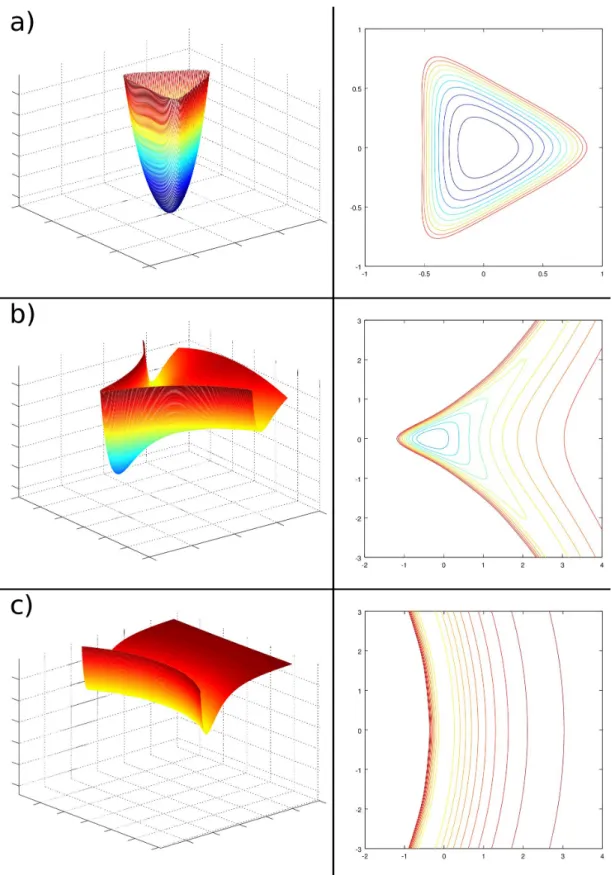
Furthermore, a deeper investigation about physical properties, led to wonder if the symmetry of the system, which is strictly bound to geometrical parameters, was capable of inducing or promoting a phase transition in the adsorbed molecules (as illustrate in figure 1.3, result of MC simulation).

(34)

Moreover, an ordered disordered phase transition has been suggested of the molecules adsorbed on graphite systems[109], but CNT systems has different symmetry. In fact any adsorbed layer has, in this case, one degree of freedom less, due to the circular conformation. At least a loss of degeneracy should be considered because, while in graphite the adsorbed layer can expand freely in two directions (planar conformation), inside CNTs only in the direction of the axis, whereas any other expansion would need to change the distance between the layer and the substrate, and, therefore , results in an increasing the energy of the system.

Such context also enlighten some issues about the insertion algorithm used in MC simulations. In these conditions, the estimation of the insertion probability converges very slowly due to the high local density and the above mentioned loss of degeneracy. Therefore, with the purpose of further developing this branch of investigation, a new algorithm has been proposed.

(35)

(36)

Chapter 2 Monte Carlo method

The question was what are the chances that a Canfield solitaire laid out with 52 cards will come out successfully?

After spending a lot of time trying to estimate them by pure combinatorial calculations, I wondered whether a more practical method than "abstract thinking" might not be to lay it out say one hundred times and simply observe and count the number of successful plays. (S. Ulam, 1946)

2.1 Historical remarks

The name Monte Carlo was suggested by Nicholas Metropolis in 1949, with explicit reference to gambling, describing a method which would use random numbers in order to study differential equations[68]. Although statistical sampling methods have long been known, only with the improvement of computational techniques it came to be feasible for complex calculations. On the basis of the law of large number and the new developments in the theory of probabilities, the method was firstly applied on neutron diffusion[107], but was soon clear that the applications would involve various branches of the natural sciences[70].

(37)

2.2 Meaning of randomness

Lots of methods and algorithms can be numbered under the category of MC; what they indeed have in common is that they make use of random numbers in order to solve complex problems. The main idea behind this approach lies into transforming a complex calculation (e.g. integration) into a matter of probabilities. An early example of such kind of situation is known as Buffon’s needle, which dates back to the 18th century. The experiment consists of tossing a needle randomly on a surface divided into stripes: the probability of the needle being in contact with the edge of a stripe can be related to the value of ﬁ. Therefore one can easily get an estimation of ﬁ by means of the frequencies. In other words, it is just like calculating the average result of a weighted dice: we could calculate an integral above the mass distribution of the dice, or simply toss it so many times that the frequency of each side is close enough to its probability.

Nevertheless, MC is not just an approximation of what analytical methods cannot easily calculate; one of its advantages is that, as long as the statistical sampling coverage is sufficient, the information gathered is not limited to average values. This means that, many times, data from a single or few simulations can be extrapolated to different conditions and produce results for a large amount of situations. The only limit is indeed the sampling, which need to be large as the extrapolation moves far from the simulation. A compromise is usually found combining multiple simulations in order to maximise the ratio between coverage and time consumed.

2.3 Monte Carlo sampling

The core of a MC simulation is undoubtedly the way how the samples are generated. Since the beginning this has been a non-trivial issue[25].

2.3.1 Uniform random numbers

Real random numbers have been obtained in several ways, measuring physical quan-tities (e.g. radioactive decays) and removing all bias which could arise from the measurement method. For instance, – decay has been used in conjunction with a high sensitive counter; the number of decays within 20ms would produce a sequence of bit, storing 0 or 1 according to whether the count was even or odd respectively[36].

(38)

Bits were then coupled and discarded if they were 1 1 or 0 0, thus correcting an eventual difference between the probabilities of generating a 0 or a 1. The couples remaining were just 1 0 or 0 1, which produce respectively 0 or 1 in the final bit sequence. Finally the bit sequence can be divided into fragments of the needed size. This way the sequence could be stored and used for calculations.

It is clear that this approach is not feasible for fast calculations, for the access to memory is a very slow process, compared with other processing capabilities. For this reason pseudo-random generator has been soon developed, where number are generated through fast and low memory-consuming algorithms, using the previous number as a seed for the next one. Since the method is thus deterministic, the sequence is reproducible, which is essential for debugging codes.

From now on the expression “random numbers” will refer to pseudo-random numbers generated within the interval [0, 1[.

2.3.2 Monte Carlo Integration

Once we have a proper set of random numbers it becomes possible to evaluate integrals using stochastic means.

Having indeed a generic function f(x) integrable within the interval [a, b], with a < b, and a uniform function g(x) defined as follows

g(x) = Y ] [ 1 b≠a if a Æ x Æ b, 0 elsewhere.

the following integral can be considered as an expectation value of f(x) with x random variable distributed according to g(x)

(b ≠ a)⁄ b

a f(x)g(x)dx (2.1)

Therefore, according to the Strong law of large numbers, the above integral can be estimated as (b ≠ a) 1 N N ÿ i=1 f(xi)

where {xi} are N random numbers in the interval [a, b] generated according to g(x).

We can therefore generalise

⁄ b a f(x)dx ƒ 1 N N ÿ i=1 f(xi) g(xi) (2.2)

(39)

where f(x), g(x) and {xi} are the same mentioned above. The symbol ƒ means that

the right part of the equation is an estimation of the value of the integral. Such estimation, although it certainly converges for N æ Œ, it will be more accurate as N increases.

Indeed if we apply the definition of the variance to the estimator we can conclude that

‡2 C ₁ N N ÿ i=1 f(xi) g(xi) D = 1 N‡ 2_{[Y ]} _(2.3)

which means that the standard deviation is proportional to 1/ÔN. In other words,

to reduce the error by ten, we need to increase the number of steps by one hundred times. Despite such drawback, MC methods have the advantage that the convergence rate does not depend, or depends very slowly, on the dimensionality of the system. This especial characteristic make this approach very useful for systems with multiple degrees of freedom.

2.3.3 Importance sampling

In many cases, sampling uniformly a multi dimensional domain is not straightforward. Usually in mathematical analysis such spaces need to be normalized, with respect to each one of the variables. It happens almost the same when trying to sample a non-squared space (i.e. a space where the domain of one variable depends on the values of any of the others). In these cases we need to correct this effect with a non uniform sampling.

Moreover, as shown in previous section (see eq. 2.3), increasing the number of steps is not an efficient way for reducing the error, although in many cases it is the only path available. A very effective way of achieving such goal is to choose the random distribution g(x) (see eq. 2.2) very similar to f(x), with the requirement that g(x) is non-zero wherever f(x) is non-zero. This improvement is especially needed if f(x) is steep and varies a lot, with zones where the function is significantly greater than in others. Knowing which are these zones would allow to sample them with higher frequency, with obvious benefits for the overall performance. Obviously the random distribution g(x) cannot be equal to f(x) because this would imply that we actually already know the integral of f(x), since it is implicit within the normalization of g(x). The sampling should be therefore studied very carefully in the light of every possible information which could somehow predict the shape of the function f(x). It should be said, nevertheless, that the choice of the sampling function g(x) does not affect the

(40)

value of the integral or of its estimate in the end, it only enhances (or not) the velocity of the convergence. In practice, it is then necessary to apply the chosen distribution to the random generator, i.e. to make it generate random numbers according to g(x).

Rejection method

One of the earliest methods was the rejection one[25]. Basically it transforms one distribution into another. Since it does not need any analytical knowledge of the sampling function it is very suitable for empirical functions or, as mentioned above, for correcting geometrical domains. So, if we are able to generate random numbers according to a specific distribution (e.g. uniform) u(x), we can convert them into any non singular distribution “(x) with the same domain, be for instance the interval [a, b]. In the first place, it should exist a real value k so that

k u(x) Ø “(x) ’x œ [a, b]

In principle k could be any value greater than max[“(x)/u(x)] however, the greater it is, the less effective the algorithm will be, since its discard rate will also be greater. Therefore k should be as low as possible in order to maximise effectiveness (see picture 2.1).

Figure 2.1: Sampling of a function f(x) with rejection method: if k is greater than the

maximum, the number of rejections is increased without any benefit (left inset); if k is not large enough the function f(x) is not sampled properly (right inset).

In the case of u(x) uniform in [0, 1[ the algorithm proceeds as follows; the generalisation is straightforward. A first random number xi is chosen in the interval [a, b[, and then

(41)

a second one “i is taken between 0 and k u(xi) xi = (b ≠ a)÷1+ a “i = k u(xi)÷2

(2.4) being ÷1 and ÷2 two random numbers in the interval [0, 1[. The i-th sample is then

considered if

“i Æ “(xi) (2.5)

otherwise is discarded. In this way the {xi} are generated according to the general

distribution “(x). Because of the presence of the k value, “(x) doesn’t even need to be normalised, thus making this method extremely useful for empirical distributions. Since the method actually samples both distributions, the acceptance rate can be used to evaluate the integral of a generic function f(x) (see eq. 2.1). The fraction of accepted samples can be an estimation of the ratio between the integrals of the two distributions, f(x) and k u(x) respectively.

Thus, if the number of samples N is sufficiently large,

⁄ b af(x)dx = k ⁄ b au(x)dx Nacc N (2.6)

the value of the integral is easily obtained by counting the number of accepted samples

Nacc, since k is known and u(x) is normalised, so its integral is actually 1.

In general the efficiency of the method depends on the acceptance rate so, besides the influence of k in increasing the rejections (see figure 2.1), sampling, for instance, a stiff peaked function with uniform distribution would result in a poor precision, or a very low convergence rate. The solution is therefore to choose a distribution

u(x), reasonably easy to sample, but also similar in shape with the function under

evaluation.

Inversion method

Another method, which does not suffer from the loss of efficiency of the rejection, consists of directly sampling according to a specific function f(x). The main disad-vantage, compared to the previous method, lies in the amount of information needed about f(x). One of the first uses of this sampling was to generate random neutron flights with an exponentially decreasing distribution[25]. Indeed, given two random variables X and Z, distributed according to u(x) and g(z) respectively, and a function

(42)

Z = f(X), all those elements are linked together by the relation: g(z) =

⁄

u(x) ” (z ≠ f(x)) dx. (2.7)

The middle term on the right side is the delta function, defined as

”(x) = Y ] [ 1 if x = 0 0 if x ”= 0. If f(X) is monotonic the integral leads to

g(z) = -dz dx -≠1 u(x(z)) (2.8)

where x(z) means the solution of the equation z = f(x) at fixed z. For the sake of completeness, if the function is not monotonic there could be more than one solution for the equation. If N solutions {xi} exist, the equation 2.8 becomes

g(z) = N ÿ i=1 1 |fÕ(x i(z))| u(xi(z)) . (2.9)

From 2.8 it is easy to see that the cumulative distribution

z = f(x) =

⁄ x

≠Œ“(t)dt (2.10)

is always a uniform random variable in the interval [0, 1[ regardless of the distribu-tion “(t). Knowing that it is possible to generate {xi} random numbers with any

distribution, as long as we can find, analytically or numerically, the solution of the equation

f(xi) = ÷i (2.11)

for each of the ÷i random numbers uniformly generated in [0, 1[. However, having to

numerically solve an equation for each random number generated will probably lead to even lower efficiency than the rejection method, and the same could happen if the analytical solution is too much complex.

For this reason it is sometimes useful to use both methods. This is possible if the main function can be expressed as f(x) = g(x)h(x) where h(x) is a function which is easy to invert and to implement. In practice random numbers {xi} are generated according

to h(x) and then selected through the rejection method if a second, uniform, random number is lower than g(xi).

(43)

2.4 Statistical thermodynamics

Once we have seen how to efficiently integrate complex functions by means of MC techniques, the main goal of this section is to present how such integrals should be, in order to properly describe macroscopic molecular behavior. A simulated system will have as many degrees of freedom as the variables which are free to change during the simulation. A miscrostate is defined as a specific configuration of all the variables of the system. Therefore, a single particle, for instance, would have 6 degrees of freedom: 3 for its position in each one of the xyz axis and the same for its momentum. All possible microstates comprise the phase space.

That said, from a macroscopic point of view, a system is composed by multiple different microstates, so that some thermodynamic properties (i.e. mechanical properties) can be calculated as an average value. This means that we can follow a statistical approach by studying microstates distribution, and therefore estimate such properties.

ÈEÍ = lim NæŒ 1 N N ÿ m=1 Em (2.12)

Thermal properties (i.e. non-mechanical) cannot be determined in such way since they depend on the whole phase space. Some methods exist[110] nevertheless, to approximate them as if they were mechanical ones.

A so called ensemble consists of a large number of replicas of the system, each one representing a microstate. They can be grouped according to one of the variables (e.g. energy), generating a statistics that shows which energies are more representative and how much. ÿ E nE N E = ÿ E fE E

Instead of summing over the microstates we are scanning all possible energies, being

nE and fE the number of states with a specific energy and its frequency, respectively.

It is straightforward that, with N sufficiently large, the frequency approaches the real probability fE æ ˝E. Of course the key point would be the coverage, because it is

unfeasible to explore the entire phase space, even for small systems, but the sample has to be large enough to be a statistically significant representation of the system under investigation (i.e. estimations do not vary too much from sample to sample). Besides, some techniques are designed to increase the sampling rate in some areas of the phase space, at the cost, of course, of the sampling in other regions[79][96]. This is usually done when some areas can be a priori excluded without being explored[97].

(44)

With discrete variables microstates are easy to handle, nevertheless, generally, many studied variables are continuous, thus making the number of microstates infinite. In these cases it is more suitable to apply the concept of density of (micro)states. The sum of 2.12, therefore, becomes an integral

ÈEÍ =

⁄ _Œ

≠Œ (E)E dE (2.13)

where E is the energy, but the same treatment could also apply to any variable that can be calculated in the microstate. (E) is the density of states (DOS), namely the fraction of states whose energies fall between E and E + dE; it is also supposed to be normalised so that _⁄

Œ

≠Œ (E)dE = 1.

Once is known, all thermodynamic properties can be obtained; however, as it happens in 2.12, we only have access to an estimation, which tends to the real value as the phase space is fully explored.

2.4.1 Ensembles

In an isolated system at equilibrium, with fixed energy, volume and particle number, each microstate is visited an equal number of times. In other words, all states accessible to the system are a priori equally probable. Entropy S(N, V, E) can therefore be calculated as a function of the DOS

S(N, V, E) = kBln (N, V, E),

being kB the Boltzmann constant. When (E) is known, as function of energy, the

above can be inverted into E(N, V, S); from there all thermodynamic properties can be calculated through partial derivative

respectively temperature, pressure and chemical potential. Such kind of ensemble is called microcanonical but, despite its straightforwardness, is not frequently used, mainly because real isolate systems are not easy to create and even less to maintain. The canonical ensemble, instead, can be visualised as a closed system (constant volume and particle number) in equilibrium with an infinite thermal bath (i.e. constant temperature). Such a system certainly resembles experimental conditions much more than the case considered above. It can be shown that the probabilities ˝m relative

(45)

to microstates with different energies, but consistent with a constant temperature, distribute according to an exponential decay

˝m = 1 Q exp 3 ≠ Em kBT 4

being kB the Boltzmann constant, T the temperature and Em the energy of the

microstate m. Since the distribution has to be normalised, the proportional constant

Q is easily calculated by the sum over all microstates m Q(N, V, T ) =ÿ m exp3≠ Em kBT 4 . (2.14)

The equation 2.14, known as the canonical partition function, is directly correlated to the characteristic thermodynamic function, which is, in this case, the Helmholtz free energy

A(N, V, T ) = ≠kbT ln(Q) (2.15)

Free energy partial derivatives then permit to obtain the other thermodynamic vari-ables. S _©1Â_ˆT2 N,V ; p© ≠ 1_Â ˆV 2 N,T ; µ© 1_Â ˆN 2 V,T .

Both partition functions (N, V, E) and Q(N, V, T ) are obtained by a sum over all possible microstates: this means scanning the whole domain of all degrees of freedom of the system. Hence, if the energy can be factorised into several independent contri-butions (in some cases it is possible to divide it into independent groups of correlated variables) this approach greatly reduces the phase space and allows to avoid useless redundancies. Such case frequently happens, for instance, when independent particles are involved: different variables are correlated only if relative to the same particle, otherwise they are considered independent. In the canonical ensemble the energy can so be divided into each particle contribution, therefore is possible to factorise the total partition function into

Q(N, V, T ) = N Ÿ i=1

qi

where qi represents each particle contribution. Besides, if N particles are

indistin-guishable, it means that N! microstates count as a single one, therefore the total partition function becomes Q = qN_/N!, where q is the partition function of a single

particle. This is also valid for multi component systems, considering each component as a different group of particles.

An open system, in equilibrium with both a thermal bath and a molecule reservoir, is consistent with the grand canonical ensemble. In terms of thermodynamic quantities,