Computational simulation of binary compounds of carbon nanotubes and amphiphilics in aqueous solution by Monte Carlo method

(1)

Computational simulation of binary compounds of carbon nanotubes

and amphiphilics in aqueous solution by Monte Carlo method

L.L. Hermsdorff

a

, C.F.S. Pinheiro

a,⇑

_{, A.T. Bernardes}

a,b a_{Dep. de Física, Univ. Federal de Ouro Preto, Ouro Preto, MG 35400-000, Brazil} b_{INMETRO, Campus Xerém, Duque de Caxias, RJ 25250-020, Brazil}

a r t i c l e

i n f o

Article history: Received 26 April 2011

Received in revised form 14 February 2012 Accepted 23 February 2012

Available online 29 March 2012

Keywords:

Monte Carlo methods Carbon nanotubes Dissociation Amphiphilics

a b s t r a c t

Carbon nanotubes have been subject of intensive research because of their outstanding physical proper-ties. The problem of dissolving the aggregation of tubes in bundles formed by strong van der Waals force is addressed in this study. A complete understanding about carbon nanotubes properties is necessary in order to obtain a process of detachment that cause no damage to the tubes. Detachment can be promoted by means of amphiphilic adsorption in water solution. We have studied this phenomenon by means Monte Carlo simulation. The algorithm used was Metropolis algorithm. The analysis of equilibrium was done by means of structure function.

1. Introduction

Since its discovery in 1991 by Iijima[1]carbon nanotubes have been the subject of intense scientific research[2]. This fact occurs due their unique properties such as electrical conduction (103A/ cm2_{), tensile strength (}

45106_{Pa), and heat transmission}

(6000 W/mK, about two times as high as diamond heat transmis-sion)[3–5]. These properties are function of the carbon nanotube morphology, which is defined by diameter and chirality of the nanotube. There is a large number of theoretical and confirmed applications in many areas of science, engineering and other areas

[6]. Nevertheless there are some difficulties in reaching this aim. A major challenge is to obtain carbon nanotubes in large quantities at low price by a feasible production method. Another difficulty is the aggregation effect of carbon nanotubes[7]. In most existent meth-ods of production many different kinds of nanotubes are produced. When in solution they are attracted by strong van der Waals forces (500 eV/

l

m per micrometer of tube-tube contact [8]) forming branches of parallel tubes. The use of carbon nanotubes in a spe-cific application depends on the separation of the nanotubes of the bundle but this is a difficult task to accomplish. An interesting approach is placing the nanotubes in a solution containing surfac-tants or polymeric structures for wrapping the CNTs and debun-dling them. Dendritic macromolecules such as PETIM can wrap CNTs and detach them, but a complex is formed altering CNT

prop-erties[9]. Many researchers have tried to promote CNT separation by means of surfactant (or amphiphilic) molecules in aqueous solution [10,7,8,11–14]. This process is inexpensive and causes no damage to the nanotube structure that could promote the loss of nanotubes properties. The knowledge about surfactant-carbon nanotube aggregation in aqueous solution process can give impor-tant information to resolve the aggregation trouble and allow the use of carbon nanotubes in various applications.

In the present work carbon nanotubes in presence of surfactant molecules in aqueous solution are simulated by Monte Carlo method in different concentrations and temperatures. Our model is bi-dimensional and off-lattice, with Larson-type particles. The algorithm used to attain the equilibrium configuration is the Metropolis Algorithm[15]. The study of the equilibrium has been done by means of the radial distribution function.

2. Model and simulation details

All molecules of our model are formed by impenetrable disks with diameterd. Each water molecule (w) is represented by a sin-gle disk. An amphiphilic molecule is represented by five disks (a head particlehand four tail particlest, making ah1t4structure)

whose centers are separated by a fixed bond distance equal tod. The angle formed by three consecutive bonded particles (or two consecutive bonds) is 109.5°(regular hexagonal lattice). For sim-plification only zig–zag helicity (8, 0) carbon nanotubes are simu-lated. The carbon nanotubes (cn) are all considered to have their axes perpendicular to the simulation plane. Therefore the

⇑ Corresponding author. Tel.: +55 31 91272528; fax:+55 31 35591667. E-mail addresses:llhermsdorff@yahoo.com.br(L.L. Hermsdorff),felpin1@gmail. com(C.F.S. Pinheiro),atb@iceb.ufop.br,atbernardes@gmail.com(A.T. Bernardes).

Contents lists available atSciVerse ScienceDirect

Computational Materials Science

(2)

nanotubes can be represented by eight disks equidistant from the nanotubes center.

Due its simplicity a water molecule moves only by translation. The amphiphilics move by translation, rotation, reptation and piv-oting (seeFig. 1). The carbon nanotubes move by rotation around its own axis and by translation.

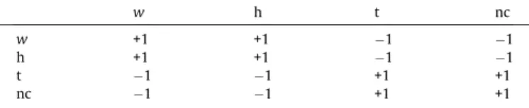
Each particle of a molecule can interact with the particles of other molecules. The configurational energy was not considered. The potential between the pairsh–h,t–t,h–w,t–cnandcn–cnare a simplification of the Lennard-Jones potential with a exclusion region of sizedand a potential well with a cut distance equal to 3d. The potential between the pairsh–t,t–w,h–ncew-nc has a exclusion region of size d and a repulsive region with size 3d. The intensity of each attraction or repulsion for these pairs isE0.

The pairw–whas a different potential with a exclusion region of sizedfollowed by a repulsion region with sizedand energy 6E0

and a E0potential well.

The potentials are represented inFig. 2. The Hamiltonian of this model is expressed in following equation

H ¼ P i;jði–jÞ

Jij

ðrÞSiSj; ð1Þ

whereris the distance between the centers of two particlesiandj, Jij_{is the intensity of the potential between these particles and}_S

iand

Sj are thei andjparticle ‘‘charges’’. The resulting product SiSjis

showed inTable 1.

All molecules are inside a square box of sizeL. The boundary conditions adopted is rigid wall. Then, if a molecule will cross the limit of the box the movement is simply rejected.

The movements are performed by first randomly choosing a molecule and then randomly choosing one of the allowed move-ments to that molecule. Then the new system energy is calculated and the Metropolis condition to the movement is analyzed. A Monte Carlo step (MCS) is defined as the number of tries to move all molecules of the system. The equilibrium is studied by means of the radial distribution function defined by[16–18]:

gðrÞ ¼

PM

k¼1Nkð~r;

D

~rÞ

M 1

2N

q

Vð~r;

D

~rÞ; ð2Þ

whereNkð~r;D~rÞis the number of molecules inside a circular layer

with internal radiusrand external radiusr+Dr,Mis the number of samples,Nis the number of molecules in the system and

q

¼NV

is the density.

3. Results and discussions

The first analysis was performed by simulating water in a box. The box size used in these simulations wasL= 40d. This size was chosen because thermalization is achieved very slowly for low

Fig. 1.Amphiphilics allowed movements. In translation, the five disks are displaced

by the same vector. In rotation, the center of a randomly chosen disk is the rotation axis. Pivoting happens by choosing a random atom and ‘‘bending’’ the molecule in that site to the other possible angle of 109.5°. In reptation, one of the ends of the molecule moves to a new allowed position so that the others follow it and move to current position of their neighbors in the chain.

(a)

(b)

(c)

Fig. 2.PotentialsJij_{adopted in our model. (}_a_{): interaction between carbon–carbon particles or amphiphilic head-water or head–head, (}_b_{): water–water interaction, (}_c_):

carbon–water interaction.

Table 1

All possibleSiSjproducts. Repulsion intensities between molecules for whichrij6dis 1(hard disk condition).

w h t nc

w +1 +1 1 1

h +1 +1 1 1

t 1 1 +1 +1

(3)

temperatures. The temperature utilized in this work is the reduced temperatureT¼kbTr

E0 whereTris the real absolute temperature,kbis the Boltzmann constant andE0is the energy of a water bond. The

amount of water in the box was chosen in order to obtain liquid-like behavior. Smaller quantities will make the system behave as a gas. As expected it was found that for lower temperatures the system had an organized structure of a solid phase, and displayed a unordered liquid behavior for higher temperatures. The structure formed whenT< 1.0 is a hexagonal lattice as seen inFig. 3a for T= 0.5. InFig. 3b we see the non-ordered structure of the liquid phase atT= 1.4. These are pictures of the system we obtained after it had reached equilibrium and they are in agreement with results found in literature[15,19].1

Fig. 4shows the radial distribution functions for water mole-cules and their corresponding Fourier transforms for T= 0.5 (a) and forT= 1.4 (b). The average separation between molecules is expected to be 2d, which is confirmed by the peaks atr 2din

Fig. 4a and b. Also, the periodicity of peaks in (a), and its absence in (b), confirms the expected distinction between ordered and unordered phases.

A second analysis was made introducing amphiphilic molecules and water in aL= 100dbox. We performed simulations in different temperatures and amphiphilic concentrations. The concentration definitions used in this work are[20]:

Xamph¼

Namph

Total volumeðLLÞ ð3Þ

Xi¼

Number of aggregates withiamphiphilics

Total volumeðLLÞ ð4Þ

Xfree

1 ¼

Number free amphiphilics

13Xamphþ3Xi ð

5Þ

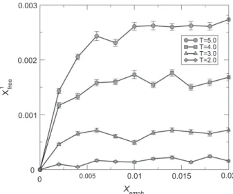
Fig. 5 showsXamphX1free curves for different temperatures. These

curves show that there is a critical micelle concentration (cmc). These results are in agreement with literature[21]. Another desired

(a)

(b)

Fig. 3.Picture of equilibrium of a system with 400 waters: (a) atT= 0.5 and(b)atT= 1.4.

0 2 4 6 8 10 n

0 0.05 0.1 0.15 0.2

Fn

20

r 0

1 2 3 4 5 6 7

g(r)

(a)

0 5 10 15 0 5 10 15 20

r 0

0.5 1 1.5 2 2.5 3

g(r)

0 2 4 6 8 10 n

0 0.02 0.04 0.06 0.08 0.1

Fn

(b)

Fig. 4.Results of radial distribution functiong(r) and Fourier transformFn(inset) for 400 water molecules after reaching equilibrium: (a) atT= 0.5 and (b) atT= 1.4.

Fig. 5.XamphX1freecurve for different temperatures.

1 _{As for a finite size system it is not possible to see a sharp phase transition, since}

infinite correlation lengths are not possible.

(4)

behavior concerns the aggregation of amphiphilics in typical surfac-tant equilibrium structures such as micelles, lamellae or vesicles. These structures were observed in our simulations. Micelles appear at small concentrations (Xamph= 0.004 in temperature T= 0.3).

Lamellae occur at medium concentration (aboveXamph= 0.006). At

this concentration micelles are elongated cylinders (cylindrical mi-celles). Vesicles have appeared only for higher concentrations (XamphP0.014). These results show that our amphiphilic model is

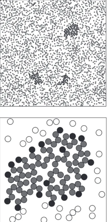
appropriate, since it agrees with results obtained by other research-ers[22]. InFig. 6we have a picture of the system after reaching equilibrium, with 2380 water molecules and 40 amphiphilics at temperatureT= 3, and the details around a micelle.

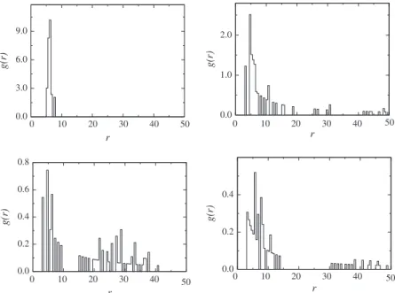
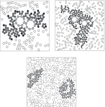
The simulations with nanotubes were carried out in aL= 100d box in presence of water and different concentrations of amphiph-ilics. Simulations with one, two and three nanotubes were performed. In simulations with 1 nanotube the aggregation of nanotubes cannot take place. Nevertheless this situation is appro-priate to study the amphiphilic-nanotube aggregate in thermal equilibrium. In small concentrations and temperatureT= 3.0 the amphiphilics form aggregates like micelles around the nanotube. An interesting phenomenon is that elongated micelles here occur at concentrations lower than before, when nanotubes were absent. This suggests that nanotubes make lamellae and vesicle formation more likely. At higher concentrations, the amphiphilics form de-formed lamellae aggregates around the nanotubes. For higher con-centrations the aggregates formed by amphiphilics are deformed vesicles.Fig. 7shows some of these structures.Fig. 8shows the re-sults of radial distribution function for different concentrations. In these curvesris the distance between an amphiphilic head and the nanotube center. Note that the curve ofXamph= 0.006 shows a high

density of amphiphilics at farther distances from nanotubes. This reveals the presence of a lamella around the carbon nanotube. TheXamph= 0.002 curve has a maximum aroundr= 6,5d. This

dis-Fig. 6.Top:picture of equilibrium of a system with 2390 water molecules and 40

amphiphilics at temperatureT= 3.Bottom:detail showing a micelle formed by 18 amphiphilic molecules.

Fig. 7.Some typical structures formed in equilibrium by amphiphilics and one carbon nanotube. Top-left: 20 amphiphilics, circular micelle-like structure; top-right: 120

(5)

tance is approximately the sum of the amphiphilic size and the nanotube radius (rnc+damphw6.3d). It shows that the amphiphilics

stand strained with the tail end near the nanotubes surface for small concentrations. In higher concentrations the maximum oc-curs at smallerr values. For these concentrations the aggregate around the nanotube is larger. This explains why the formation of a strained configuration of amphiphilics is more difficult.

Fig. 9shows the results of the radial distribution function aver-aged over 40 samples obtained after thermal equilibrium. These images show some peaks aroundr= 2.5 meaning the amphiphilic head is near the nanotube surface. According to the hamiltonian describing the system, that is an unfavorable energetic situation. This result suggests that the nanotube deforms the amphiphilic aggregate when it penetrates the aggregate. These amphiphilics

stand in this situation and cannot easily change their configuration.

Fig. 10shows pictures of the thermal equilibrium with different kinds of aggregates. At T= 4.0 the system behaves similarly to T= 3.0 only for higher amphiphilics concentrations. At temperature T= 5.0 the amphiphilics do not form aggregates around the nanotubes.

The simulations with two nanotubes always started with nano-tubes placed touching each other. In aqueous solution without amphiphilics the nanotubes do not dissociate. Dissociation process will only take place when the nanotubes do not interact with each other, which occurs for distances greater than 3d. Then two nano-tubes are dissociated when the minor distance between a particle of one nanotube and a particle of the other nanotube is greater than 3d. At temperature T= 3.0 dissociation does not occur for

50

r 0.0

3.0 6.0 9.0

g(r)

50 r

0.0 1.0 2.0

g(r)

50 r

0.0 0.2 0.4 0.6 0.8

g(r)

0 10 20 30 40 0 10 20 30 40

0 10 20 30 40 0 10 20 30 40 50 r

0.0 0.2 0.4

g(r)

Fig. 8.Radial distribution function for systems with 20, 40, 60 and 80 amphiphilics.

r 0.0

1.0 2.0 3.0

g(r)

50

r 0.0

0.5 1.0 1.5

g(r)

50 r

0.0 0.2 0.4

g(r)

0 10 20 30 40 0 10 20 30 40

0 10 20 30 40 0 10 20 30 40 50 r

0.0 0.2 0.4

g(r)

50

Fig. 9.Radial distribution function for systems with 20 (top-left), 40 (top-right), 60 (bottom-left) and 80 (bottom-right) amphiphilics. These curves correspond to averages

over 40 samples.

(6)

small concentrations. In our simulations withXamph= 0.006, there

is enough amphiphilic to form an aggregate that could cause sep-aration, yet the aggregates that are formed are not bulky enough. Only for concentrations above Xamph= 0.008 dissociation occurs.

In all simulation withXamphP0.008 carbon nanotube dissociation

was observed. In higher amphiphilics concentrations vesicles ap-pear in the system and the nanotubes stay inside the vesicles.

In simulations with 3 nanotubes the same concentration thresholds were observed for dissociation. At concentrations below Xamph= 0.008 the nanotubes stay together. This implies the

deter-minant factor for this dissociation is the capacity of the amphiph-ilics to form big enough aggregates. In other words this capacity is determined by the number or fraction of amphiphilics in the sys-tem. This result has already been reported in a recent experimental work[23].

4. Conclusions

The separation of carbon nanotubes from the bundles of tubes by use of amphiphilic molecules in aqueous solution was studied with Monte Carlo Simulation. Our model actually showed some characteristics of this detachment. Detachment only took place for larger amphiphilic concentrations. The determinant character-istic that defines the detachment in our model is the capacity of the formation of big aggregates of amphiphilic molecules around the nanotubes. The amphiphilics surrounding the nanotubes are responsible for this detachment. This detachment process is suit-able given its simplicity concerning materials, not to mention the low costs involved. Nevertheless, this process does not destroy or modify the nanotubes structure, keeping their properties intact. With our model we found that the concentration of amphiphilics in the system defines how effective is the detachment of carbon nanotubes, which is corroborated by recent experimental results

[23].

Acknowledgments

The authors are thankful to the national agencies Fapemig, CNPq and Capes for financial support.

References

[1] S. Iijima, Nature 354 (1991) 56–58, doi:10.1038/354056a0.

[2] G. Mountrichas, N. Tagmatarchis, S. Pispas, The Journal of Physical Chemistry B 111 (29) (2007) 8369–8372, doi:10.1021/jp067500k (pMID: 1738845). [3] D. Tomanek, Preface and introduction, in: A. Jorio, M. Dresselhaus, G.

Dresselhaus (Eds.), Carbon Nanotubes: Advanced Topics in the Synthesis, Structure, Properties and Applications, Topics in Applied Physics, vol. 111, Springer, Berlin, 2008.

[4] P.G. Collins, P. Avouris, Scientific American 283 (2000) 62–69.

[5] R.H. Baughman, A.A. Zakhidov, W.A. de Heer, Science 297 (5582) (2002) 787– 792, doi:10.1126/science.1060928.

[6] J. Chen, M.A. Hamon, H. Hu, Y. Chen, A.M. Rao, P.C. Eklund, R.C. Haddon, Science 282 (5386) (1998) 95–98, doi:10.1126/science.282.5386.95. arXiv:http:// www.sciencemag.org/content/282/5386/95.full.pdf, URL <http:// www.sciencemag.org/content/282/5386/95.abstract>.

[7] V.A. Sinani, M.K. Gheith, A.A. Yaroslavov, A.A. Rakhnyanskaya, K. Sun, A.A. Mamedov, J.P. Wicksted, N.A. Kotov, Journal of the American Chemical Society 127 (10) (2005) 3463–3472, doi:10.1021/ja045670.

[8] M.J. O’Connell, S.M. Bachilo, C.B. Huffman, V.C. Moore, M.S. Strano, E.H. Haroz, K.L. Rialon, P.J. Boul, W.H. Noon, C. Kittrell, J. Ma, R.H. Hauge, R.B. Weisman, R.E. Smalley, Science 297 (5581) (2002) 593–596, doi:10.1126/science.1072631. [9] G. Jayamurugan, K.S. Vasu, Y.B.R.D. Rajesh, S. Kumar, V. Vasumathi, P.K. Maiti,

A.K. Sood, N. Jayaraman, The Journal of Chemical Physics 134 (10) (2011) 104507, doi:10.1063/1.3561308. URL <http://link.aip.org/link/?JCP/134/ 104507/1>.

[10] B. Koh, J.B. Park, X. Hou, W. Cheng, The Journal of Physical Chemistry B 115 (11) (2011) 2627–2633, doi:10.1021/jp110376h. arXiv:http://pubs.acs.org/ doi/pdf/10.1021/jp110376, URl <http://pubs.acs.org/doi/abs/10.1021/ jp110376h>.

[11] R. Duggal, M. Pasquali, Physical Review Letters 96 (24) (2006) 246104, doi:10.1103/PhysRevLett.96.246104.

[12] Y. Kang, T.A. Taton, Journal of the American Chemical Society 125 (19) (2003) 5650–5651, doi:10.1021/ja034082d (pMID: 1273390).

[13] R. Bandyopadhyaya, E. Nativ-Roth, O. Regev, R. Yerushalmi-Rozen, Nano Letters 2 (1) (2002) 25–28, doi:10.1021/nl010065f.

[14] S. Bhattacharyya, J.-P. Salvetat, D. Roy, V. Heresanu, P. Launois, M.-L. Saboungi, Chemical Communications (2007) 4248–4250, doi:10.1039/B709499J. URlL <http://dx.doi.org/10.1039/B709499J>.

(7)

[15] E. Teller, N. Metropolis, A. Rosenbluth, Journal of Chemical Physics 21 (13) (1953) 1087–1092.

[16] N. Metropolis, A.W. Rosenbluth, M.N. Rosenbluth, A.H. Teller, E. Teller, Journal of Chemical Physics 21 (1953) 1087–1092.

[17] A.T. Bernardes, T.B. Liverpool, D. Stauffer, Physical Review E 54 (3) (1996) R2220–R2223, doi:10.1103/PhysRevE.54.R2220.

[18] T. Megyes, S. Bálint, I. Bakó, T. Grósz, T. Radnai, G. Pálinkás, Chemical Physics 327 (2-3) (2006) 415–426, doi:10.1016/j.chemphys.2006.05.014.

[19] A. Lehninger, D. Nelson, M. Cox, et al., Principles of Biochemistry, Worth Publishers, New York, 1982.

[20] A.T. Bernardes, V.B. Henriques, P.M. Bisch, The Journal of Chemical Physics 101 (1) (1994) 645–650, doi:10.1063/1.468120.

[21] S. Yang, X. Zhang, S. Yuan, Journal of Molecular Modeling 14 (2008) 607–620, doi:10.1007/s00894-008-0319-7. URL <http://dx.doi.org/10.1007/s00894-008-0319-7>.

[22] E.D. Goddard, G.C. Benson, Transactions of the Faraday Society 52 (1956) 409– 413, doi:10.1039/TF9565200409.

[23] A.J. Blanch, C.E. Lenehan, J.S. Quinton, The Journal of Physical Chemistry B 114 (30) (2010) 9805–9811, doi:10.1021/jp104113d.