Unsteady Parallel Flows (Plate Suddenly Set in Motion)

Exact Solutions to the Navier-Stokes Equation

Unsteady Parallel Flows (Plate Suddenly Set in Motion)

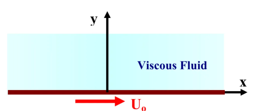
Consider that special case of a viscous fluid near a wall that is set suddenly in motion as shown in Figure 1. The unsteady Navier-Stokes reduces to

2 2

y u t

u ∂ ∂ ν = ∂ ∂

(1)

U

o

Viscous Fluid

y

x

Figure 1. Schematics of flow near a wall suddenly set in motion. The boundary conditions are:

At y=0 u=U₀ (2)

at y=∞, u=0 (3)

The corresponding initial condition for the fluid that starts from rest is given as

at t =0 u=0. (4)

Similarity Solution (Group Theory)

Let

, (5)

1

t ~

t , y~ta

Equation (1) implies that

,

a 2

Thus,

2 1

t ~

y (7)

Now introducing the similarity variables

t 2

y ν =

η , =f

( )

η U

u

0

, (8)

we find t 2 1 u y u ν η ∂ ∂ = ∂ ∂ , t 4 1 u y u 2 2 2 2 ν η ∂ ∂ = ∂ ∂ (9) t 2 u t 2 1 t 2 y u t u η η ∂ ∂ − =      − ν η ∂ ∂ = ∂ ∂

. (10)

Substituting (9) and (10) in Equation (1), we find

t 4 1 f t 2 f ν ′′ ν = η ′

− , (11)

or

0 f 2

f ′′+ η ′= (12)

Boundary and initial conditions (2)-(4) in terms of the similarity variables become 1

) 0 (

f = , f(∞)=0. (13)

From Equation (12), it follows that η − = ′ ′′ 2 f f

, or lnf′=lnc−η2 (14)

or

, and , (15)

2 ce

f′= −η f c e d 1

0 1

2

1 η +

where the first boundary condition in (13) is used. The second boundary condition implies that

( )

_∫

∞ _−η

η +

= = ∞

0 e d 1

c 1 0

f 21 _or

π − = η −

∫

∞ −η

2

d e

1

0 1

2 1

=

c (16)

Equation (15) then becomes

( )

η − = η π

−

=

_∫

η −η

erf 1 d e 2 1 f

0 1

2

1 ₍₁₇₎

or

η =erfc

f , _

  

 

ν =

t 2

y erfc U

u ₀ (18)

Time variations of the velocity profile as predicted by Equation (18) are shown in Figure 2.

Transform Method

0

0.0

0.2

0.4

0.6

0.8

1.0

u/Uo

0.5

1

1.5

2

2.5

3

y

Figure 2. Time variations of velocity profile.

tν=4

tν=1

tν =0.25

An alternative is to use the transform method. Taking Laplace transform of Equation (1), it follows that

2 2

y u u

s

∂ ∂ ν

= (19)

or

0 u s

u =

ν − ″

(20)

The solution to (20) is

y s y

s

Be Ae

u= − ν + ν (21)

Boundary conditions (2) and (3) imply that

s U

A= 0 _{, B}=_{0 (22)}

Thus, the solution in the transform domain is given by

y s 0 _e

s U

u= − ν (23)

Inverse Laplace transform of (23) gives

   

 

ν =

t 2

y erfc U

u ₀ . (24)

Oscillating Plate

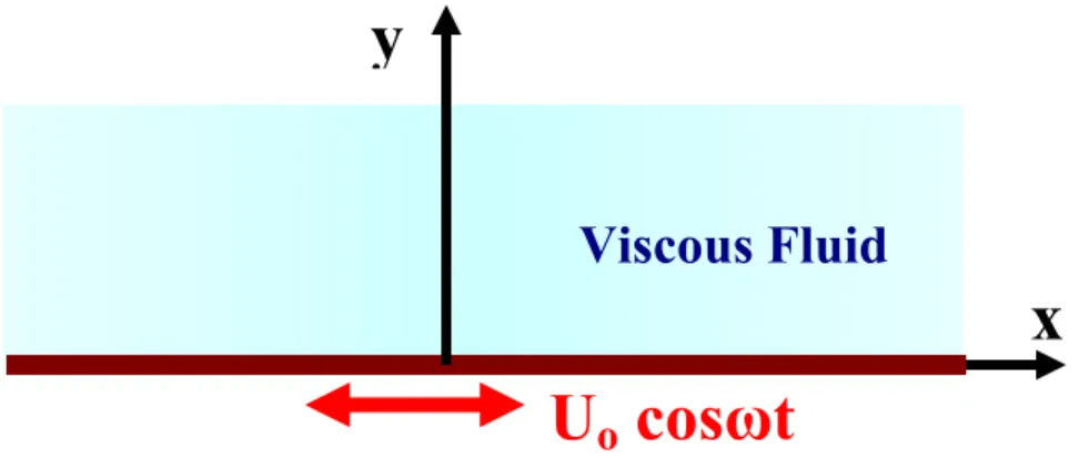
Consider that case of a viscous fluid near an oscillating wall as shown in Figure 3. The unsteady Navier-Stokes reduces to

2 2

y u t

u ∂ ∂ ν = ∂ ∂

U

o

cos

ω

t

Viscous Fluid

y

x

Figure 2. Schematics of flow near an oscillating wall. The boundary conditions are:

t at cos

U

u= ₀ ω y=0 (26)

at

0

=

u y=∞ (27)

Let

(

t ay cos

e U

u= ₀ −ky ω −

)

. (28)

Then

(

t ay sin

e

U

)

t

u ky

0 ω −

ω − = ∂

∂ −

(29)

(

)

(

(

kcos t ay asin t ay e

U y

u ky

0 − ω − + ω −

= ∂

∂ −

))

(30)

(

θ− θ− θ

= ∂

∂ −

cos a sin ka 2 cos k e U y

u ky 2 2

0 2 2

)

, ayθ=ωt− (31)

Substituting (29)-(31) into Equation (25) it follows that

(

)

(

− θ− θ

)

ν = θ ω

− sin k2 a2 cos 2aksin ₍₃₂₎

2 2

k

a = (33)

ν = ν =

ω 2

k 2 ak

2 (34)

a 2

k =

ν ω

= (35)

Thus, the velocity profile is given as

(

t ky

)

cos e U

u= ₀ −ky ω − ,

ν ω =

2

k . (36)

Unsteady Flow in a Tube

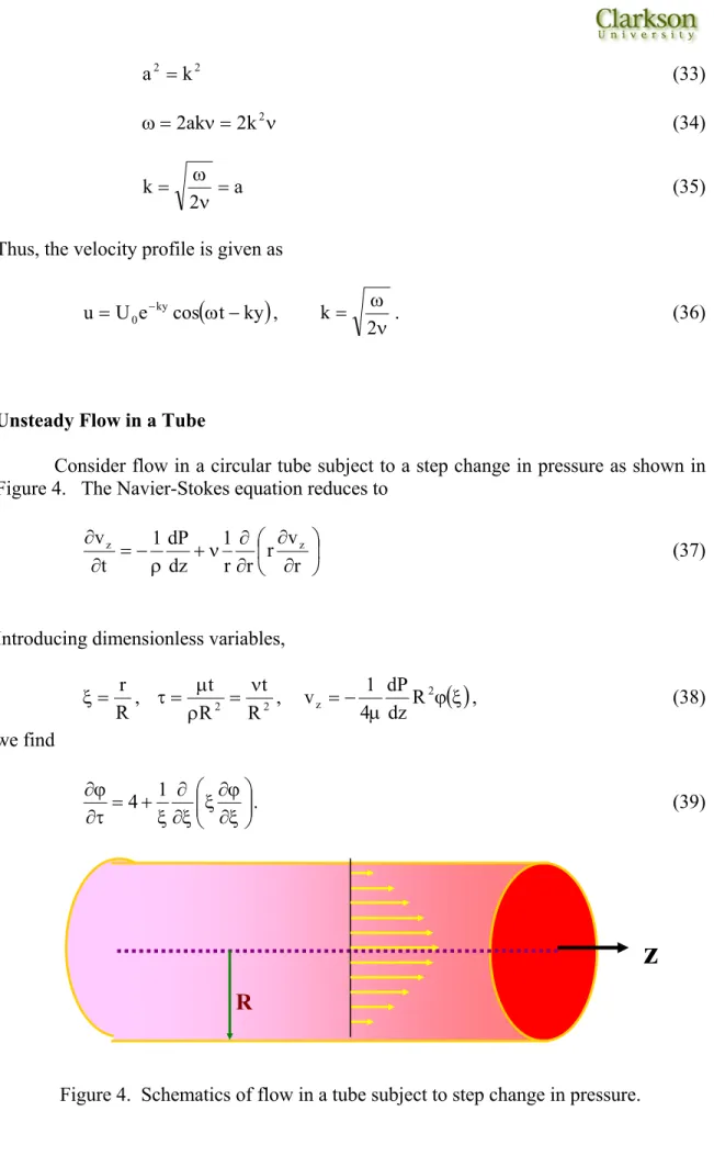
Consider flow in a circular tube subject to a step change in pressure as shown in Figure 4. The Navier-Stokes equation reduces to

     

∂ ∂ ∂

∂ ν + ρ − = ∂ ∂

r v r r r 1 dz dP 1 t

v_{z z}

(37)

Introducing dimensionless variables,

R r =

ξ , _{2 2}

R t R

t ν

= ρ

µ =

τ , ϕ

( )

ξ

µ −

= 2

z R

dz dP 4

1

v , (38)

we find

     

ξ ∂

ϕ ∂ ξ ξ ∂

∂ ξ + = τ ∂

ϕ

∂ 1

4 . (39)

R

z

The boundary condition is

0 at , (40)

=

ϕ ξ=1

with the initial conditions

0 at . (41)

=

ϕ τ=0

Let

, (42)

ψ − ξ − =

φ 2

1

Equation (39) reduces to

     

ξ ∂

ψ ∂ ξ ξ ∂

∂ ξ = τ ∂

ψ

∂ 1

(43)

The boundary and initial conditions (40) and (41) now become

At ξ=1, ψ =0. (44)

At τ=0, ψ =1−ξ2. (45)

To find the solution the method of separation of variable is used. That is let

(46)

( ) ( )

ξ τ =

ψ F T

Equation (43) then becomes

2

d dF d

d F

1 T

T _=−α

     

ξ ξ ξ ξ = &

. (47)

From Equation (47), it follows that

0 , (48)

0 F d dF d F

d 2 2

2 2

2 +α ξ =

ξ ξ + ξ

ξ . (49)

The solutions to Equations (48) and (49) are given as

(50) τ α − = 2 Ce T

, (51)

( )

αξ +

(

αξ =AJ₀ BY₀

F

)

)

)

where J₀

(

αξ and Y₀

(

αξ are Bessel function of first and second kind of zeroth order. The boundary conditions are

since

( )

0 ~finite B 0

F ⇒ = Y₀

( )

0 →∞. (52)

and

. (53)

( )

1 0 J

( )

0

F = ⇒ ₀ α =

Equation (53) is a characteristic equation. The corresponding eigenvalues, α_n, are given as

405 . 2

1 =

α , α₂ =5.52, α₃ =8.654,… (54)

The general solution for Equation (43) then is given by

(55)

(

∑

α ξ

=

ψ −ατ

n

n 0

ne J

A 2n

)

)

Using the initial condition

(55)

(

∑

α ξ = ξ − n n 0 n 2 J A 1 then

(

)

( )

( )

( )

( )

n 2 1 3 n n 1 1 0 n 2 0 1

0 0 n

2 n J 5 . 0 / J 4 d J d J 1 A α α α = ξ ξ α ξ ξ ξ α ξ ξ − =

∫

∫

(56) or

( )

_n

1 3 n n J 8 A α α

= . (57)

( )

( )

∑

_{α α}α ξ

=

ψ −ατ

n 1 n

3 n

n 0

J J e 8

2 n

, (58)

and

( )

( )

∑

−ατ

α α

ξ α −

ξ − = ϕ

n 1 n

3 n

n 0

2 _e n

J J 8

1 (59)

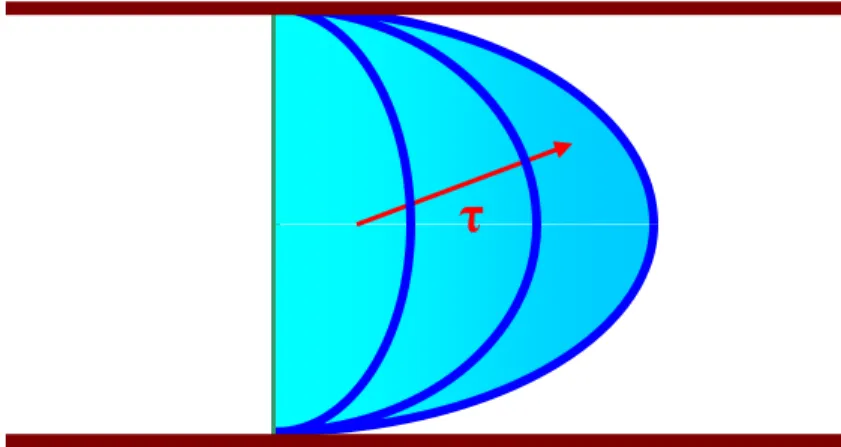
Variation of the velocity profile in the pipe is shown schematically in Figure 5.

Figure 5. Variations of velocity field in a tube subject to a step change in pressure.

Noncircular Pipe Flows

Consider steady state viscous flows in a pipe with arbitrary cross section under a constant pressure gradient as shown in Figure 6. The Navier-Stokes equation is given as

const dz

dP 1 W

2 =

µ =

∇ . (60)

The corresponding boundary condition is

on S. (61)

0 W=

S

Figure 6. An arbitrary cross-section pipe subject to a constant pressure gradient.

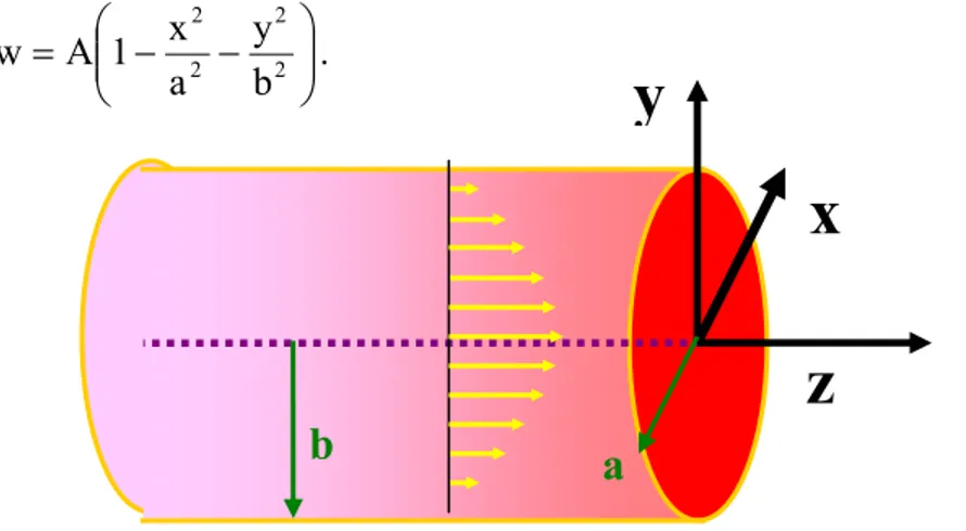
Elliptical Pipes

Consider an elliptical cross-section pipe shown in Figure 7 with its boundary given as

1 b y a

x 2 2 ₌

      +      

. (62)

We assume that the velocity field is given by

   

 

− −

= ₂2 ₂2

b y a x 1 A

w . (63)

a

y

x

z

b

(

)

dz dP 1 b

a b a A 2 b

2 a

2 A

w _{2 2}

2 2 2

2 2

µ = + −

=    



 ₊

− =

∇ (64)

Hence

   

 

− − +

µ −

= ₂2 2_{2 2}2 ₂2

b y a x 1 b a

b a dz dP 2

1

A (65)

The flow rate is given as

. (66)

∫∫

= wdxdy

Q

After integration, it follows that

2 2

3 3

b a

b a dz dP 4 Q

+ µ

π −

= . (67)

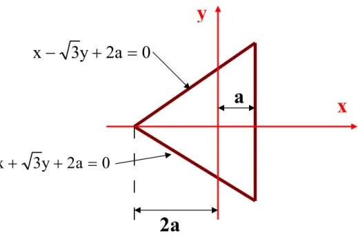
Triangular Pipes

Consider a pipe as shown in Figure 8 whose cross section is an equilateral triangle. The equation of the section is given as

( ) (

x,y x a

)

(

x 3y 2a

)(

x 3y 2a

)

0

f = − − + + + = . (68)

Assuming

(69)

(

x,y Af

w=

)

Then

( )

dz dP 1 aA 12 y , x f A

w 2

2

µ = =

∇ =

0

a

2

y

3

x

+

+

=

0

a

2

y

3

x

−

+

=

2a

a

y

x

Figure 8. A triangular pipe subject to a constant pressure gradient.

Thus,

dx dP a 12

1 A

µ

= (71)

Hence,

(

x a

)

(

x 3y 2a

)(

x 3y 2a

)

dx

dP a 12

1

w − − + + +

µ