J. Braz. Soc. Mech. Sci. & Eng. vol.25 número4

A. L. Braun

PPGEC/UFRGS Av. Osvaldo Aranha, 99 – 3o andar 90035-190 Porto Alegre, RS. Brazil www.cpgec.ufrgs.br [email protected]

A. M. Awruch

PPGEC/UFRGS & PROMEC/UFRGS Av. Sarmento Leite, 425 90050-170 Porto Alegre, RS. Brazil www.mecanica.ufrgs.br/promec [email protected]

Numerical Simulation of the Wind

Action on a Long-Span Bridge Deck

Keywords: Fluid-structure interaction, Finite Element Method (FEM), Large Eddy Simulation (LES), aeroelasticity, aerodynamics

Introduction

Wind tunnel tests for assessment of aerodynamic and aeroelastic informations in the study of bridge girders performance are numerically simulated in this work. The usual way to obtain these informations is using representative models in a wind tunnel. However, with the improvement in computers technology and computational fluid dynamics (CFD) algorithms, many of these problems can also be analyzed by numerical simulation.1

Long-span bridges, such as suspension bridges for example, must be designed to support, from a static point of view, the mean wind forces (using the drag, lift and pitching moment coefficients). Besides, considering that such structures show low damping and low stiffness, they are subjected to aeroelastic phenomena, such as flutter, galloping and vortex shedding induced vibrations. Only the first case will be studied in the present work.

The term aeroelasticity is used when the aerodynamic forces produce some kind of structural instability as a consequence of the interaction between these forces and the structural motion. The flutter phenomenon is a type of aeroelastic instability that begins when the effective damping (structural + aerodynamic) becomes negative.

Kawahara & Hirano (1983) were one of the first authors to analyze numerically the wind action on a bridge cross-section. They used the Finite Element Method (FEM) to obtain the aerodynamic coefficients as functions of the angle of attack of the wind and the Strouhal number.Kuroda (1997) employed two different numerical procedures to study the approaching span of the Great Belt East Bridge: the Finite Element Method and the Finite Difference Method (FDM), and Large Eddy Simulation (LES) with the Smagorinsky’s model for the turbulent flow. He also presented the results referring to the aerodynamic coefficients for various angles of attack and the Strouhal number for both numerical methods employed in his analysis. Larsen & Walther (1997) analyzed several bridge decks observing their aeroelastic behaviour using a numerical code based on Discrete Vortex Simulation (DVS), presenting the respective critical flutter velocity (using the flutter derivatives). Recently,Selvam et al. (2002) applied a direct method for the flutter analysis. They used (FEM) and (LES).

In this work, the analysis of the flow of a slightly compressible fluid in a two-dimensional flow domain was carried out using an

Paper accepted August, 2003. Technical Editor: Aristeu da Silveira Neto..

explicit two-step Taylor-Galerkin method with an Arbitrary Lagrangean-Eulerian (ALE) description. A similar Taylor-Galerkin formulation was used byTabarrok & Su (1994) and byRossa & Awruch (2001), but with a semi-implicit scheme. The (ALE) scheme was first presented byHirt et al. (1974) in a numerical work. Since this first paper many other authors used this description with the same concepts. The classical Smagorinsky’s model, similar to that presented byKuroda (1997), was employed for the sub-grid scales simulation. The finite element method was used for spatial discretization. The structure was considered as a rigid body with elastic restrains for the cross-section rotation and displacement components. The coupling between fluid and structure was performed applying the compatibility and equilibrium equations at the interface. The structural dynamic analysis was accomplished using the classical Newmark’s method (Bathe, 1996). Examples are presented to illustrate the capability of the computational method.

Governing Equations for the Flow Simulation

The governing equations, considering the pseudo-compressibility approach in an isothermic process, Large Eddy Simulation (LES) with Smagorinsky’s model for turbulent flows and an Arbitrary Lagrangean-Eulerian (ALE) description, are:

a) Momentum equations:

(

)

(

)

    

  

∂ ∂ +     

  

∂ ∂ + ∂ ∂ + ∂

∂ − ∂

∂ + ∂ ∂ − + ∂ ∂

ij k k

j i

i j t j ij j j i j j i

x v x v x v

x x

p x v w v t

v _{δ ν ν λ δ}

ρ

(i, j, k = 1, 2) in Ù (1)

being νt =

(

)

(

)

  

∂ ∂ + ∂ ∂ =

i j

j i

ij _x

v x v S

2 1

and

(

)

Ä= 1/2, whereÄx andÄy are the element dimensions in the global axis direction x and y, respectively.

b) Mass conservation equation:

(

)

∂ ∂ + ∂

∂ − + ∂ ∂

j j

j j j

x v c x

p w v t p

ρ (j = 1, 2) in Ù (2)

which is obtained considering∂p_∂ρ=c2.

i

i w

v = (i = 1, 2) on the solid boundary S

v

à (3)

vˆ

v= on the boundary a

v

à or p

ˆ

p= on the boundary Ã_p (4)

(

)

j ij j k k i j j i t

ij _ñ S

n ó n x v ë x v x v í í ä ñ p = =         ∂ ∂ +         ∂ ∂ + ∂ ∂ + + −

(i,j,k=1,2) in Ã_ó (5)

In these equations, v_i and p (the velocity components and the pressure, respectively) are the unknowns. The viscosities

ñ ì í= and ñ ÷

ë= , the specific massñ and the sound velocityc, are the fluid properties. The eddy viscosity

ñ ì

í t

t= depends of

derivatives of the filtered velocity components, of the element dimensions and of the Smagorinsky’s constant C_S. For a purely Eulerian description, the mesh motion velocity w at each nodal point, with components w_i, is equal to zero. Now, for a purely Lagrangean description, the mesh motion velocity at each nodal point is equal to the fluid velocity, i.e. v_i=w_i (i = 1, 2). Finally, in an Arbitrary Lagrangean-Eulerian formulation, w≠0 and w≠v.

On the boundaries a

v

à and Ã_p, prescribed values for velocity and pressure, vˆ and ˆp, respectively, must be specified, while on

ó

à the boundary force tˆ must be in equilibrium with the stress tensor components ó_ij. In Eq. (5), n_j is the direction cosine between a vector perpendicular to Ã_ó and the axis x_j.

Initial conditions for the pressure and the velocity components at t = 0 must be given.

The Algorithm for the Flow Simulation

Expanding the governing equations in a Taylor’s series up to second order terms, the algorithm for the flow simulation contains the following steps (Braun, 2002):

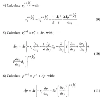
1) Calculate n+12 i

v~ with:

    ∂ ∂       +         ∂ ∂ +         ∂ ∂ + ∂ ∂ ∂ ∂     + ∂ ∂ − ∂ ∂ − + = + k j n i k j n ij k k i j j i j ij j j i j n i n i x x v r r t Ä ä x v ë x v x v í x ä x p ñ x v r t Ä v v~ 2 2 1 4 1 2 (6)

whererj=(vj−wj) and v=(ν +νt). 2) Calculate _pn+12 _with:

    ∂ ∂ ∂       +             ∂ ∂ − ∂ ∂ − + = + i j n j i n j j j j n n x x p r r t Ä x v c ñ x p r t Ä p p 2 2 2 1 4 2 (7)

3) Calculate Äpn+12=pn+12−pn_{. (8)}

4) Calculate n+12 i

v with:

i n n i n i _x p Ä t Ä ñ v~ v ∂ ∂ − = + +

+ 2 12

2 1 2 1 8 1 (9)

5) Calculate v_in+1=v_in+Äv_i with:

2 1 1 +        ∂ ∂     +         ∂ ∂ + ∂ ∂ ∂ ∂     + ∂ ∂ − ∂ ∂ − = n ij k k i j j i j ij j j i j i ä x v ë x v x v í x ä x p ñ x v r t Ä v Ä (10)

6) Calculate pn+1=pn+Äp with:

2 1 2 +                 ∂ ∂ − ∂ ∂ − = n j j j j x v c ñ x p r t Ä p Ä (11)

These expressions must be employed after applying the classical Galerkin technique into the finite element method (MEF) context.

As the scheme is explicit, the resulting system is conditionally stable, with a stability condition given by:

i i i v c x Ä á t Ä +

< (i = 1,...,NTE) (12)

where á (which is a real number less than one) is a safety coefficient, Äx_i and v_i are the i-th element characteristic dimension and the velocity, respectively, and NTE is the total number of elements.

Although variable time step could be adopted (Teixeira & Awrucha, 2001), in this work an unique value of Ät will be used for the whole process, adopting the smallest one from those obtained by Eq. (12).

The Fluid-Structure Coupling

In the present work, the structure is idealized as a two-dimensional rigid body. Displacement and rotations take place on the plane formed by the axis x1 and x2; the body is restricted by

dampers and springs, as indicated in Fig. 1.

Figure 1. Structure model, formed by a rigid body restricted by springs

and dampers. Structure degrees of freedom:u₁ = displacement in the

direction of axis x₁.u₂ = displacement in the direction of axisx₂. è =

rotation around the axisx₃ (perpendicular to the plane formed by the axes

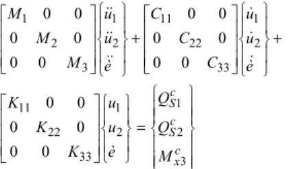
The structural dynamic equilibrium equation is given by the following matrix expression:

c S ~ c S ~ S ~ c S ~ S ~ c S ~ S ~ Q U K U C U

M + + = (13)

where

S ~

M is the mass matrix,

S ~

Cthe damping matrix,

S ~

K the

stiffness matrix and c

S ~ c S ~ U ,

U and c

S ~

U the acceleration, velocity and

generalized displacements, respectively. Finally, c

S ~

Q is the load vector.

The subscript S means that these matrices belong to the structure and the superscriptC indicates that these values correspond to the gravity center of the solid body. Equation (13) can be written as follows:             =                     +                     +                     c x c S c S M Q Q è u u K K K è u u C C C è u u M M M 3 2 1 2 1 33 22 11 2 1 33 22 11 2 1 3 2 1 0 0 0 0 0 0 0 0 0 0 0 0 0 0 0 0 0 0 (14)

It must be noticed that the hypothesis of a rigid structure is proper when deformations of the cross-section are small compared to the rotation and displacement components.

At the solid-fluid interface, the compatibility condition must be satisfied, or in other words, the fluid velocity and the structure velocity must be the same at the common nodes of both fields. The compatibility condition and the translation of variables evaluated at the center of gravity of the body to a point located at the fluid-structure interface may be written with the following expressions:

c S ~ ~ I F ~ I S ~ U L V

U = = with _

     − = 1 2 1 0 0 1 l l L ~ (15)

where S and F are referred to the structure and the fluid, respectively, and the superscriptI is referred to the interface. It is important to notice that the both vectors I

S ~

U and I

F ~

V have two components that correspond to the global axis direction. However,

c

S ~

U has three components, because it includes the rotation around an axis perpendicular to the plane formed byx1 andx2. Values of

c

S ~

U can be transported to the solid-fluid interface (or to nodes belonging to the structure boundary) through a translation matrix

~

L, as given by Eq. (15), being l1 and l2 the distance components

between the gravity center of the body and the point under consideration, measured in the global system. Considering Fig. 2, it is observed that the distance components from a boundary point to the body gravity center are functions ofè, and it may be written as follows: A g ~ ~ A g A g

~ _x Rx

x è cos è sen è sen è cos ) è ( l ) è ( l ) è ( l =               − =       = 2 1 2 1 ₍₁₆₎

Deriving Eq. (15) with respect to time, taking into account matrix

~

L and equation (16), the following expression is obtained:

c S ~ ~ c S ~ ~ I F ~ I S ~ U ) è ( ' L U L V

U = = + , where

        − − = è l è l ) è ( ' L ~ 2 1 0 0 0 0 (17)

Equation (15) and Eq. (17) are applied to each node at the interface, where the equilibrium condition must be also satisfied, that means that the load

~

S acting on the structure at the interface, must be equal to the load

~

S given by Eq. (5), but with an opposite signal (because here the fluid action on the structure is considered, while Eq. (5) represents the boundary action on the fluid).

~

S can be transported to the center of gravity of the body, obtaining:

à d S L Q S à ~ T ~ c S ~

∫

L is the transpose matrix of

~

L, given by Eq. (15), and

~

S contains the two components of the fluid boundary force acting on the structure at a point located on the structure surface ÃS (ÃS represents also the solid-fluid interface); these forces

~

S are given by Eq. (5), but with an opposite signal.

X

x

C

A'

l

C'

l

l

x

l

X

A

X

~

_x

x

x

l

l

l

=

















=

















=

Figure 2. Rigid body motion. The subscripts “g” and “l” are referred to quantities related to global and local axis, respectively.

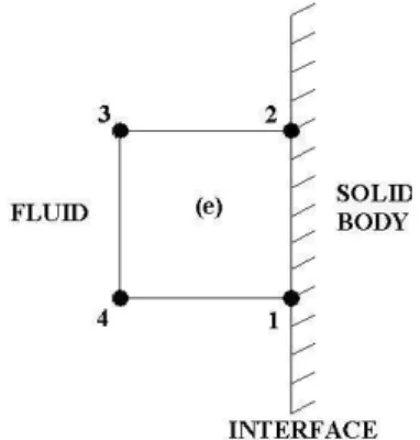
Figure 3. Element of the fluid domain in contact with the solid body.

The momentum equations in its matricial form, at element level (e), can be obtained by applying the Galerkin method to the Eq. (1), writting:           +           =                     +                       F ~ I ~ F ~ I ~ F ~ I ~ FF ~ FI ~ IF ~ II ~ F ~ I ~ FF ~ FI ~ IF ~ II ~ S S GP GP ñ V V AD AD AD AD V V MM MM MM MM 1 (19) where ~

MM contains the time derivative coefficients from the velocity components

~

V,

~

AD contains the coefficients of advective and diffusive terms,

~

GP contains the coefficients of pressure derivative terms with respect to x1 and x2 and, finally,

~

S is a vector containing the boundary integrals resulting from the integration by parts of pressure and diffusive terms.

In Eq. (19), I

~

V and I

~

V contain, respectively, acceleration and velocity components corresponding to nodes 1 and 2 of Fig. 3, while

F

~

V and VF

~

contain variables corresponding to nodes 3 and 4 of

the same figure. A similar remark can be made with respect to the vectors of pressure gradients

~

GP and boundary forces

~

S. Matrix

II

~

MM contains elements coming from the connection of node 1 with itself and with node 2, and the connection of node 2 with itself

and with node 1. Matrix IF

~

MM reflects the connection between the nodes 1 with 4 and 2 with 3. Similar commentaries can be made

with respect to matrices II

~

AD and IF

~

AD .

Regarding the structural analysis, only the first matricial expression of Eq. (19) is necessary, because only this equation contributes to the assembling of the overall dynamic equilibrium equation. On the other hand, as the structural and the flow analysis are performed in a sequential form in this work, the system constituted by the solid body and fluid elements with one or more sides common to the solid-fluid interface have prescribed values of

~

V and

~

P at nodes that do not have any contact with the structure

(they were calculated previously in the flow analysis). Referring to

Fig. 3, at nodes 3 and 4, the values F

~

V and F

~

P are known. All these considerations lead to the elimination of the second expression of Eq. (19) when the governing equations which describe the solid body motion are built, taking into account the solid-fluid coupling effect. The first expression of Eq. (19) can be re-written as:

I ~ I ~ F ~ IF ~ F ~ IF ~ I ~ II ~ I ~ II

~ V AD V MM V AD V ñGP S

MM + + + −1 = (20)

Equation (15) with matrix

~

L and Eq. (17) with matrix L'(è)

~

are considered for each node at the interface. Then, when an element side with two nodes and lying on the fluid-structure interface is considered, Eq (15) and Eq. (17) are written in the following form:

c S ~ ~ I ~ I S ~ U T V

U = = ; c

S ~ ~ c S ~ ~ I ~ I S ~ U ) è ( ' T U T V

U = = + (21)

Referring again to Fig. 3, the matrices

~

T and '

~

T are given by:

          =                 − − − − =           =                 − − = ) è ( L ) è ( L è l l l l ) è ( ' T ; L L l l l l T ' ~ ' ~ ~ ~ ~ ~ 2 2 2 1 1 2 1 1 2 1 2 2 1 1 1 2 0 0 0 0 0 0 0 0 1 0 0 1 1 0 0 1 (22)

The contribution from I

~

S , on the side 1-2 of the element (e), to the total load acting at the gravity center of the body, can be calculated as: I ~ T ~ c

S T S

Qˆ =− (23)

Considering Eqs. (14), (15), (17) and (20), with the last one multiplied by ñ, the structural dynamic equilibrium equation, taking into account the solid-fluid coupling effect, is given by:

        + ∑ _ + − _ − = +       ∑ _ + _ + +       ∑ _ _ + = = = c S NTL i i I T F IF T F IF T c S S c S NTL i i II T II T S c S NTL i i II T S Q GP T V AD T V MM T U K U T MM T T AD T C U T MM T M ~ ~ ~ ~ ~ ~ ~ ~ ~ ~ ~ ~ ~ ~ ~ ~ ~ ~ ~ ~ ~ ~ ~ ~ ' 1 1 1 ρ ρ ρ ρ ρ (24)

whereNTL is the total number of fluid elements in contact with the structure, having at least one straight segment common to the solid body surface, forming the solid-fluid interface. The matricial Eq. (24) is re-written as:

c S ~ c S ~ S ~ c S ~ S ~ c S ~ S

~ U C U K U Q

As can be noticed,

S ~

C is a non-symmetric matrix, because it

contains the advective terms and

  

_{T MM T'(è)}

~ II ~ T ~

. This last term

leads to the non-linearity of matrix S ~

C .

In this work, a monolithic coupling between fluid and structure was not considered. The analysis for both fields is made in a sequential way. Firstly, Eq. (6) to Eq. (11) are solved, with the smallest Ät calculated with Eq. (12) and applying the boundary conditions given by Eq. (3) to Eq. (5). After, Eq. (25) is solved using the Newmark’s method (Bathe, 1996). Although different time steps may be used for the fluid and the structure, here the same time step was adopted, because the computer time required by the structure analysis is negligible with respect to the processing time demanded by the flow analysis. Furthermore, compatibility and equilibrium conditions are more accurately imposed if the same time intervals are employed.

Strouhal Number and Aerodynamic Coefficients Calculation

The Strouhal number (St) can be calculated with

0 0

V L f St= v , whereV0 is a reference velocity,L0 a reference dimension and fv is the shedding frequency of a pair of vortices. It depends of the immersed prism cross-section, its oscillations, its superficial details, the Reynolds number and the flow characteristics. Formulation to calculate this number is presented in many publications and texts (for example,Schlichting, 1979). When the Strouhal number of a flow with a given immersed structure is known, it is possible to obtain the velocity V_0R, which will produce the resonant phenomenon on the vibrating body. It occurs when the shedding frequency of a pair of vortices is approximately equal to the structural natural frequency.

The drag coefficient CD is related to the acting forces on the structure in the flow direction, while the lift coefficient CL is related to the acting forces on the structure in the transversal-to-flow direction. Finally, the pitching moment coefficientCM is related to the torsional moment acting at the gravity center of the immersed prism. The three coefficients can be calculated using the following expressions:

0 2 0 1

1

2 1

L V ñ

S C

NTN

i i I

D

∑

= ;

0 2 0 1

2

2 1

L V ñ

S

C NTN

i i I

L

∑

= ;

(

)

(

)

1 2 2 1

2 1

L V

l S l S C

NTN

i i i

I i i I

M

ρ + −

=

∑

(26)

where S₁I and S₂I are the forces in the directions x1 and x2,

respectively, acting on the structure at node i, located on the interface. l_1i and l_2i are the projections in the directions x1 and x2,

respectively, of the distance between the gravity center and nodei. NTN is the total number of nodes located on the solid-fluid interface. The forces S₁I and S₂I are the components of the force vector I

~

S , given by Eq. (20). These forces are applied to the structure on each fluid element side belonging to the interface.

The pressure coefficient at a point i, Ci_p, located on the interface, is related to the pressure acting at that point. This coefficient can be calculated using the following expression:

2 0

0

2 1

V ñ

P P

Ci_p = i− (27)

wherePi is the pressure at nodei and P0 is a reference pressure (for example, the pressure in an undisturbed area of the flow). With the instantaneous values of pressure coefficients, the time history may be obtained and then the mean pressure distribution on the body surface, for a given time interval, may be calculated.

The Automatic Mesh Motion Scheme

Taking into account that the immersed body in the fluid can move and rotate in its plane and that the flow is described by an Arbitrary Lagrangean-Eulerian (ALE) formulation, a scheme for the mesh motion is necessary, establishing the velocity field w in the fluid domain, such that the element distortion will be as smaller as possible, according to the following boundary conditions:

=

erface int

w I

E ~ I

F

~ U

V = ;

~ boundaries external

w =0 (28)

In the present work, the mesh motion scheme is similar to that used byTeixeira & Awruchb _{(2001). Considering thati is an inner}

point in the fluid field andj is a boundary node, the mesh velocity components at node i , in the direction of the axis xk, are given by:

∑

∑

= = = _NS

j ij NS

j j k ij i k

a w a

w

1

1 _{(k = 1, 2) (29)}

whereNS is the total number of nodes belonging to the boundary lines andaij are the influence coefficients between the inner points and the boundary lines of the flow field, being

( )

d

a = 1 , where

dij is the distance between i and j, and n≥1. The exponent n can be adjusted by the user. Although regions with purely Eulerian and purely Lagrangean descriptions mat be used simultaneously with the ALE formulation, this alternative may result in more complex and less efficient codes. It may also lead to more difficulties to control mesh distortions.

Examples

Analysis of the Flow Around a Rectangular Prism

This example presents a prism with a rectangular cross-section free to oscillate in the transversal-to-flow and rotational directions. Through this problem, the program performance for large and coupled motion is observed, even that this cross-section form is not usually employed in bridge structures. In this study, special attention is given to the structural dynamic response in the two degrees of freedom of the cross-section and to the finite element mesh motion, remembering that a special scheme is employed for the non-linear dependence with respect to the cross-section rotation in the compatibility condition at the solid-fluid interface.

a non-dimensional form, are shown in Fig. 4. In addition, initial velocity and pressure field for the fluid-structure interaction problem are those of a developed flow obtained with a fixed body.

Figure 4. Flow around a rectangular prism: geometry and boundary conditions.

The finite element mesh has 5865 nodes and 5700 quadrilateral bi-linear isoparametric elements and is shown in Fig. 5. A

non-dimensional time step Ät∗ = 1.0x10-4 was adopted. The fluid and structural data are presented in Table 1.

Table 1. Rectangular prism: dimensionless data for the fluid and the structure.

Rectangular Prism - Reynolds 1000

Specific mass (ñ) 1.0

Volumetric viscosity (ë) 0.0

Reynolds number (Re) 1000

Mach number (M) 0.06

Reference/inflow velocity (V0) 1.0

F

lu

id

d

ata

Characteristic dimension (D) 1.0

Dimensionless longitudinal stiffness (K*

11) 3x104

Dimensionless transversal stiffness (K *

22) 0.7864

Dimensionless torsional stiffness (K *

33) 17.05

Dimensionless longitudinal mass (M*

1) 195.57

Dimensionless transversal mass (M *

2) 195.57

Dimensionless torsional mass (M *

3) 105.94

Dimensionless longitudinal damping (C*

11) 1x107

Dimensionless transversal damping (C *

22) 0.0325

S

tr

u

c

tu

r

al

d

ata

Dimensionless torsional damping (C *

33) 0.0

X

Y

0 2 4 6 8 10 12 14 16 18 20 22 24

0 1 2 3 4 5 6 7 8 9 10

Figure 5. Rectangular prism: finite element mesh.

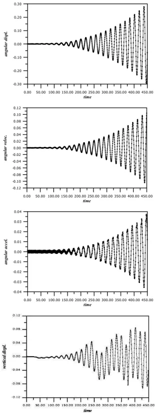
In Fig. 6 the time histories related to angular and vertical displacements, velocities and accelerations are presented. It is important to notice that the time used in these figures is dimensionless. These results are very similar to those obtained by Sarrate et al. (2001), using a different method.

0.00 50.00100.00 150.00 200.00 250.00 300.00 350.00 400.00 450.00 time

-0.30 -0.20 -0.10 0.00 0.10 0.20 0.30

an

gu

la

r

d

is

pl

.

0.00 50.00100.00 150.00 200.00 250.00 300.00 350.00 400.00 450.00 time

-0.12 -0.10 -0.08 -0.06 -0.04 -0.02 0.00 0.02 0.04 0.06 0.08 0.10 0.12

an

gu

la

r

ve

loc

.

0.00 50.00100.00 150.00 200.00 250.00 300.00 350.00 400.00 450.00 time

-0.04 -0.03 -0.02 -0.01 0.00 0.01 0.02 0.03 0.04

an

gu

la

r

a

cc

el

.

0.00 50.00100.00 150.00 200.00 250.00 300.00 350.00 400.00 450.00 time

-0.04 -0.03 -0.02 -0.01 0.00 0.01 0.02 0.03 0.04

ve

rt

ic

a

l

ve

lo

c.

0.00 50.00100.00 150.00 200.00 250.00 300.00 350.00 400.00 450.00 time

-0.015 -0.010 -0.005 0.000 0.005 0.010 0.015

ve

rt

ic

a

l

ac

ce

l.

Figure 6. (ontinued).

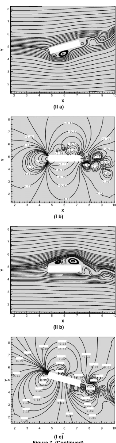
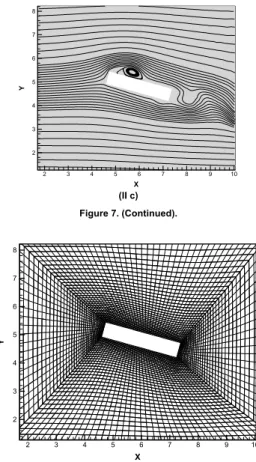
The streamlines and the pressure field are shown in Fig. 7, in three instants (t* = 439, t* = 442 and t* = 448). It can be observed the presence of high pressure gradients and large vortices alternating between the lower and the higher surfaces. The streamlines show that the cross-section orientation with respect to the free flow direction modifies the boundary layer form. This conclusion is the same observed in bluff bodies, where the flux-ward dimension is one of the parameters that determine the forms of the boundary layer and wake. In Fig. 8 it is verified the distortion of the mesh in an instant where extreme structural rotation is reached.

0.15

0.16 0.18

0.23 0.31 0.40

-0.15 -0.18 -0.32 -0.58

-0.10 -0.05

-0.02 0.00 0.02 0.04

0.05 0.11

0.06

0.05

0.02 0.11

-0.05 -0.02 0.00 -0.32

-0.58 -0.02

-1.94

0.07

0.14 -0.15

X

Y

2 3 4 5 6 7 8 9 10

2 3 4 5 6 7 8

(I a)

Figure 7. Rectangular prism: (I) pressure contours and (II) streamlines contours; (a) t* = 439; (b) t* = 442 and (c) t* = 448.

X

Y

2 3 4 5 6 7 8 9 10

2 3 4 5 6 7 8

(II a)

-0.23 -0.16

-0.10

-0.05

-0.02

0.00 -0.02

0.05

0.03 0.03

0.05 0.16

0.07

-0.72

-0.58

-0.02

0.02 0.02

-0.16 -1.63

-0.02 -0.05

0.07 0.11

0.16

X

Y

2 3 4 5 6 7 8 9 10

2 3 4 5 6 7 8

(I b)

X

Y

2 3 4 5 6 7 8 9 10

2 3 4 5 6 7 8

(II b)

-0.18

-0.32

-0.58

-1.94 -0.10

-0.05 -0.02

0.23

0.18 0.16

0.15

0.14 0.00

0.05 -0.10

0.11

0.11 0.00

0.02

0.04 -0.58 0.07

-0.05 0.31

0.40

0.07

0.00 -0.15

-0.18

X

Y

2 3 4 5 6 7 8 9 10

2 3 4 5 6 7 8

X

Y

2 3 4 5 6 7 8 9 10

2 3 4 5 6 7 8

(II c)

Figure 7. (Continued).

X

Y

2 3 4 5 6 7 8 9 10

2 3 4 5 6 7 8

Figure 8. Rectangular prism: finite element mesh at t* = 448.

It can be observed that a satisfactory performance has been obtained for this example. The ability of the code to study fluid-structure interaction problems, where immersed bodies move due to the flow action with large displacements and rotations was also confirmed. In addition, the main characteristics of flows around bluff bodies were well simulated. The analysis of this kind of problem is only possible if a special Arbitrary Lagrangean-Eulerian (ALE) description is used. Another important aspect that is the mesh motion model, used previously byTeixeira & Awrucha _{(2001), was}

applied here with the same success.

Numerical Study of the Great Belt East Bridge Cross-section

In this section, results of the numerical simulation of the wind action on a cross-section belonging to the Great Belt East Bridge are presented, including the aerodynamic and the aeroelastic behavior. The studies are accomplished by fixed and oscillating sectional models, according to the usual wind tunnel techniques.

The Great Belt East Bridge is located in Denmark, precisely in the Great Belt Channel, an important international shipping route. The design phase was initiated in 1989, being it opened to the traffic in 1998. It is a suspension bridge, with a superstructure constituted by two approaching spans of 535 m (each one) and a central span of 1624 m, which will be studied in this work. In Fig. 9, general aspects of the bridge are shown. The pictures were taken from Larsen & Walther (1997).

(a)

(b)

Figure 9. General characteristics of the Great Belt East Bridge: (a) cross-section; (b) elevation.

Firstly, the fixed cross-section was analyzed and the aerodynamic coefficients were obtained as functions of the angle of attack of the wind direction. The Strouhal number was also calculated. Finally, free oscillations of the cross-section in the vertical and the rotational degrees of freedom were allowed in order to carry out dynamic instability investigations.

Analysis of the Flow Around the Fixed Cross-Section

The computational domain and the boundary conditions used in this example, are illustrated in Fig. 10. As can be noticed, the inflow boundary conditions are functions of the angle of attack of the wind direction. Four different values of the angle of attack were studied: -10º, -5º, 0º e +5º. The initial pressure and velocity were assumed equal to zero.

Figure 10. Great Belt East Bridge: geometry and boundary conditions for the fixed cross-section.

The finite element mesh employed in this problem has 8175 bilinear isoparametric elements with 8400 nodes, and is shown in Fig. 11.

X

Y

0 50 100 150 200 250

0 10 20 30 40 50 60 70 80 90

The Reynolds number used in the four cases is 3.0x105. The other constants used in the analysis are presented in Table 2. From the well-known Courant stability condition, the time step isÄt = 1.15x10-4 s.

Table 2. Great Belt East Bridge: data used to determine aerodynamic coefficients.

Constants

Great Belt East Bridge -Reynolds 3x105 Specific mass (ñ) 1.32 Kg/m3 Volumetric viscosity (ë) 0.0 m2/s

Kinematic viscosity (í) 5.78x10-4 m2/s

Sound velocity (c) 337.0 m/s

Reference/inflow velocity (V0) 40.0 m/s Smagorinsky’s constant (CS) 0.2 Charact. dimension/cross-section(D) 4.40 m

The investigated mean coefficients, obtained from the time histories, are plotted in Fig. 12 as functions of the angle of attack, and compared with the experimental results given by Reinhold et al. (1992) and the numerical results obtained by Kuroda (1997).

-10.00 -5.00 0.00 5.00 10.00

angle of attack(degrees) -1.20

-1.00 -0.80 -0.60 -0.40 -0.20 0.00 0.20 0.40 0.60 0.80 1.00

CD

,C

L

a

n

d

CM

Present work

Reinhold et al. (1992) - (exp.)

Kuroda (1997) - (num.) CD

CL

CM

Figure 12. Great Belt East Bridge: numerical and experimental results for aerodynamic coefficients as functions of the angle of attack.

The Strouhal number, obtained from the vertical velocity component time history V2 at a point located a distance 0.2 B behind

the cross-section (with zero angle of attack), is 0.18. Comparisons of some of the results obtained for Strouhal number of the referred bridge are shown in Table 3.

Table 3. Strouhal number for the Great Belt East Bridge.

Reference

Strouhal number - Reynolds 3x105

Present work 0.180

Larsen et al. (1998) (numer.) 0.170 Wind tunnel tests (from: Larsen et al. (1998)) 0.160

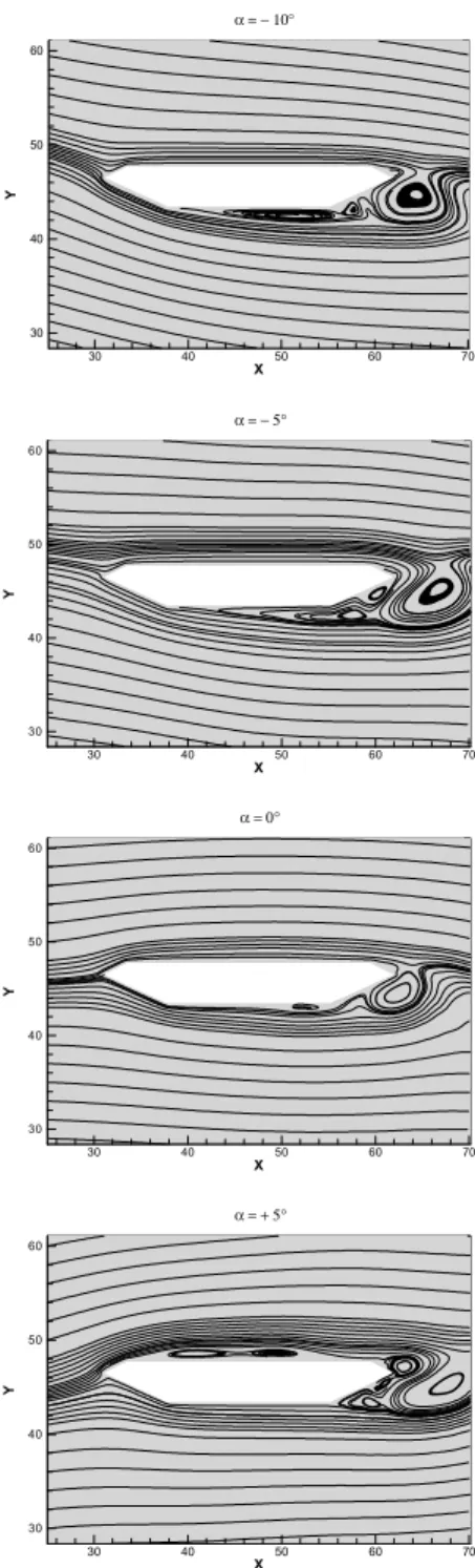
The streamlines observed for the different angles of attack are presented in Fig. 13 and are similar to those obtained byKuroda (1997).

X

Y

30 40 50 60 70

30 40 50 60

α = − 10°

X

Y

30 40 50 60 70

30 40 50 60

α = − 5°

X

Y

30 40 50 60 70

30 40 50 60

α = 0°

X

Y

30 40 50 60 70

30 40 50 60

α = + 5°

Figure 13. Great Belt East Bridge: streamlines contours for different angles of attack.

Aeroelastic Analysis: Flutter

In Selvam et al. (2002), it is shown a method in which the growth/decay rate is determined from the structural response,

observed in several reduced wind velocities given by

B f V

V∗₌ 0 _,

whereV0 is the inflow velocity,B is the bridge deck width andf is

the natural structural frequency. These values of the growth/decay

rate are calculated with ã_g/d =(yk−yk+1) yk, whereyk _{and y}k+1

are the peak values in the same oscillation period. After, they are transported to a chart in function of the reduced wind velocity, and the critical velocity corresponds to the point where the curve crosses the velocity axis (growth/decay rate = 0).

In the flutter derivatives method (Scanlan & Tomko, 1971), the experimental damping æ_èexp and the natural frequency ù_èexp for each reduced wind velocity are obtained from the structural response. These values are introduced into an expression, representing the aerodynamic damping and given by:

( )

  

  

−

= exp

è exp è

è è *

* _æ

ù ù æ B ñ

I V

A₂ 4₄ (30)

whereI is the mass moment of inertia,ñ is the specific mass of the fluid, B is the bridge deck width, æ_è is the structural critical damping and ù_è the structural natural frequency. Eq. (30) may be also written, by experimental considerations, in a reduced

expression in terms of the logarithmic decrement äexp ≅2ðæexp as follows:

( )

B ñ

I V A

exp è *

* 2

4

2 =− (31)

Thus, a curve of this coefficient A*₂ in function of the reduced wind velocities is built. The critical flutter velocity is obtained by a critical condition expressed by:

B ñ

æ I

A*₂=4 è (32)

So, when A*₂>4Iæ_è ñB the aerodynamic damping is greater than the structural damping, originating negative damping and oscillations with growing amplitudes.

The geometry as well as the finite element mesh employed in the determination of the critical velocity of flutter is the same that was used previously (Fig. 10 and Fig. 11). Initially, a fixed cross-section with an inclination of 1.8º was taken. After 30000 time steps, the load boundary conditions at the body surface were computed, and then, the body motion was allowed. The outflow boundary conditions were kept identical to the case where the body remains fixed with zero angle of attack, with exception to the inflow velocity, which changes in order to obtain the desired curves.

The physical properties and design values of the structure, employed in the experiments, are found in Table 4. The structure is idealized such that only torsional rotations are allowed (because it was verified that coupling vertical displacements and rotations will not modify significativelly the critical velocity of flutter).

The problem was analyzed for four reduced velocities: 2, 4, 6 and 10. These values correspond to the following inflow velocities: 16.86 m/s, 33.73 m/s, 50.59 m/s and 84.32 m/s, respectively. The flow was analyzed with Re = 105_.

Table 4. Great Belt East Bridge: structural data used in the flutter analysis.

Great Belt East Bridge – Reynolds 105– Structural data Longit. and transv. stiffness (K11, K 22) 3x109 N/m.m

Torsional stiffness (K 33) 7.21x106 N.m/rad.m Longit. and transv. mass (M1, M 2) 2.27x104 N.s2/m.m

Torsional mass (M 3) 2.47x106 N.m.s2/rad.m Longit. and transv. damping (C11, C 22) 3x104 N.s/m.m

Torsional damping (C 33) 0.00 N.m.s/rad.m Vertical natural frequency (fh) 0.099 Hz Angular natural frequency (fè) 0.272 Hz

Critical damping (æ) 0.002

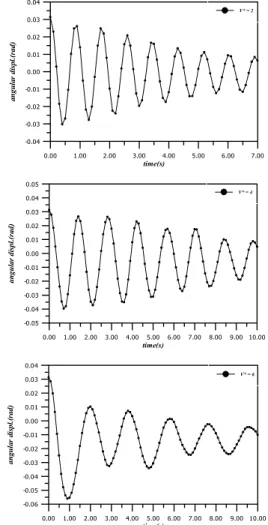
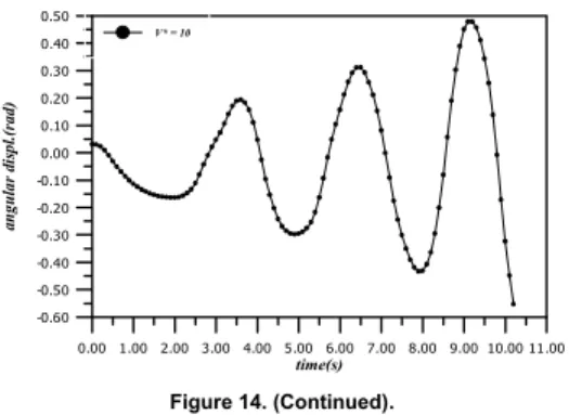
In Fig. 14, time histories related to the angular displacement are presented for each reduced wind velocity. From the rotation time histories, the growth/decay rate as well as the logarithmic decrement for each reduced velocity were obtained. In Table 5 all these values are presented.

0.00 1.00 2.00 3.00 4.00 5.00 6.00 7.00

time(s)

-0.04 -0.03 -0.02 -0.01 0.00 0.01 0.02 0.03 0.04

an

g

u

la

r

d

is

pl

.(

ra

d

)

V* = 2

0.00 1.00 2.00 3.00 4.00 5.00 6.00 7.00 8.00 9.00 10.00

time(s)

-0.05 -0.04 -0.03 -0.02 -0.01 0.00 0.01 0.02 0.03 0.04 0.05

an

gu

la

r

d

is

p

l.

(r

a

d)

V* = 4

0.00 1.00 2.00 3.00 4.00 5.00 6.00 7.00 8.00 9.00 10.00

time(s)

-0.06 -0.05 -0.04 -0.03 -0.02 -0.01 0.00 0.01 0.02 0.03 0.04

an

g

u

la

r

d

is

pl

.(

ra

d)

V* = 6

0.00 1.00 2.00 3.00 4.00 5.00 6.00 7.00 8.00 9.00 10.00 11.00

time(s)

-0.60 -0.50 -0.40 -0.30 -0.20 -0.10 0.00 0.10 0.20 0.30 0.40 0.50

a

n

gu

la

r

d

is

pl

.(

ra

d)

V* = 10

Figure 14. (Continued).

Table 5. Great Belt East Bridge: numerical results for flutter analysis.

Great Belt East Bridge - Reynolds 105

Results

V* = 2 V* = 4 V* = 6 V* = 10 Growth/decay rate 0.131 0.270 0.311 -0.500 Logarithmic decrement 0.176 0.205 0.291 -0.403

In Fig. 15 the curves to obtain the critical velocity of flutter by the direct method of Selvam et al. (2002) and by the flutter derivative A*₂ (Scanlan & Tomko, 1971), respectively, are presented.

0.00 2.00 4.00 6.00 8.00 10.00

V*=V/fB -0.20

-0.15 -0.10 -0.05 0.00 0.05 0.10 0.15 0.20

A*

2

A*2 = 0.0162

(a)

0.00 2.00 4.00 6.00 8.00 10.00

V*=V/fB -2.00

-1.80 -1.60 -1.40 -1.20 -1.00 -0.80 -0.60 -0.40 -0.20 0.00 0.20 0.40 0.60 0.80 1.00 1.20 1.40 1.60 1.80 2.00

G

ro

w

th

/d

ec

a

y

ra

te

(b)

Figure 15. Flutter analysis: (a) by the flutter derivative *

2

A and (b) by the

direct method for the Great Belt East Bridge.

From Fig. 15, the reduced critical velocity obtained by the direct method is 8.18, corresponding to a velocity of 69 m/s. By the flutter

derivative method, considering the critical condition as A*2 ≥

1.62x10-2, yields a reduced velocity equal to 8.66 which corresponds to a critical velocity equal to 73 m/s. In Table 6 below, comparisons of the critical velocity obtained by this work and by other authors (through numerical and experimental works) are shown.

Table 6. Flutter velocity for the Great Belt East Bridge.

Great Belt East Bridge – Flutter velocity

Reference Vcrit(m/s)

Present work – direct method 69 Present work – flutter derivative 73 Selvam et al. (2002) (num.) 65-72 Larsen et al. (1997) (num.) 74 Enevoldsen et al. (1999) (num.) 70-80 Wind tunnel tests (from: Larsen et al. (1998)) 73

Conclusions

A model for the numerical simulation of the wind action on bridges was described. The computational code was validated through the analysis of a rectangular cross-section and studies of the aerodynamic and aeroelastic behavior of the Great Belt East Bridge cross-section. The results show good agreement with those obtained by other authors. In future works, it is expected to explore other bridge decks, considering details such as cables, guardrails and aerodynamic appendages. It is also expected improvements in the efficiency in processing time, mainly in turbulent flows. An alternative is to use time integration with subcycles (Teixeira & Awrucha_{, 2001), optimizing the time step on the computational}

domain. Another possibility is to use semi-implicit schemes for the flow analysis.

References

Bathe, K. J. Finite Element Procedures. Prentice Hall, Englewood

Cliffs, NJ, 1996.

Braun, A. L. “A Numerical Model for the Simulation of the Wind Action on Bridge Cross-Sections” (In Portuguese), Msc. Thesis, Federal University of Rio Grande do Sul, Porto Alegre, R.S., Brazil, 2002, 139p.

Enevoldsen, I.; Pederson, C.; Hansen, S. O.; Thorbek, L. T. & Kvamsdal, T. Computational wind simulations for cable-supported bridges.

Wind Engineering into the 21st _{Century, Vol.2}

, pp. 1265-1270, 1999.

Hirt, C. W.; Amsden, A. A. & Cook, J. L. An arbitrary Lagrangean-Eulerian computing method for all flow speeds. Journal of Computational Physics, V.14, pp. 227-253, 1974.

Kawahara, M. & Hirano, H. A finite element method for high Reynolds number viscous fluid flow using two step explicit scheme. International Journal for Numerical Methods in Fluids, V.3, pp. 137-163, 1983.

Kuroda, S. Numerical simulation of flow around a box girder of a long span suspension bridge. Journal of Wind Engineering and Industrial Aerodynamics, V.67&68, pp. 239-252, 1997.

Larsen, A. & Walther, J. H. Aeroelastic analysis of bridge girder sections based on discrete vortex simulation. Journal of Wind Engineering and Industrial Aerodynamics, V.67&68, pp. 253-265, 1997.

Larsen, A. & Walther, J. H. Discrete vortex simulation of flow around five generic bridge deck sections. Journal of Wind Engineering and Industrial Aerodynamics, V.77&78, pp. 591-602, 1998.

Rossa, A. L. & Awruch, A. M. 3-D finite element analysis of

incompressible flows with heat transfer. Proceedings of the 2nd

International Conference on Computational Heat and Mass Transfer, COPPE/UFRJ,, Rio de Janeiro, Brazil, pp. 22-26, October, 2001.

Reinhold, T. A.; Brinch, M. & Damsgaard, A. Wind tunnel tests for the Great Belt link. In: Proceedings International Symposium on Aerodynamics of Large Bridge, pp. 255-267, 1992.

Sarrate, J.; Huerta, A. & Donea, J. Arbitrary Lagrangean-Eulerian

formulation for fluid-rigid body interaction. Computer Methods in Applied Mechanics and Engineering, V.190, pp. 3171-3188, 2001.

Schlichting, H. Boundary-Layer Theory. McGraw-Hill Inc., New York, 2nd

ed., 1978, 815 p.

Selvam, R. P.; Govindaswamy, S. & Bosch, H. Aeroelastic analysis of bridges using FEM and moving grids. Wind and Structures, V.5, pp. 25-266, 2002.

Tabarrok, B. & Su, J. Semi-implicit Taylor-Galerkin finite element method for incompressible viscous flows. Computer Methods in Applied Mechanics and Engineering, V.117, pp. 391-410, 1994.

a

Teixeira, P. R. F. & Awruch, A. M. Three dimensional simulation of high compressible flows using a multi-time-step integration technique with subcycles. Applied Mathematic Modeling, V.25, pp. 613-627, 2001.

b

Teixeira, P. R. F. & Awruch, A. M. Analysis of compressible fluids and elastic structures interaction by the finite element method. Proceedings

of the 16th