The population genomics of western Iberian Squalius freshwater fish species: a genotyping by sequencing approach

(1)

UNIVERSIDADE DE LISBOA

FACULDADE DE CIÊNCIAS

DEPARTAMENTO DE BIOLOGIA ANIMAL

The population genomics of western Iberian Squalius

freshwater fish species: a genotyping by sequencing approach

Sofia Lopes Mendes

Mestrado em Biologia Evolutiva e do Desenvolvimento

Dissertação orientada por:

Professor Doutor Vítor Sousa

Professora Doutora Maria Manuela Coelho

(2)

(3)

Acknowledgments

First, I would like to thank both my supervisors, for accepting me as their student, trusting me with this project and being the most amazing supervisors anyone can wish for. To professor Manuela, thank you for introducing me to the beauty of evolution and especially to the beauty of freshwater fish. To Vítor, thank you for the incredible amount of patience and for introducing me to the world of bioin-formatics. Thank you both for your guidance, support, encouragement and for giving me the opportunity to learn so much and grow, both in science and as a person.

To all my colleagues in the Evolutionary Genetics group for providing such a great work envi-ronment and especially to João, Carlos and Cátia, who were conducting their master dissertations at the same time, for making this such an enjoyable year. I would also like to thank Miguel Machado for the helpful suggestions and discussion regarding the analysis of paired-end GBS data.

To all my friends, for their support and encouragement. In particular, to my friend Mariana, for sharing her accomplishments and frustrations with me and listening to mine, no matter how small some problems might seem now. Thank you for sharing this journey with me since the first day at FCUL. To my friend Margarida, for being such an example of positivity and perseverance. To my friend Marta, for always being here, throughout the good and the bad.

To Nuno, for being such a support. Thank you for your patience and encouragement and for believing in me when I didn’t.

A toda a minha família, por ter sempre acreditado em mim. Ao meu pai, por trabalhar todos os dias para que eu pudesse chegar aqui. À minha mãe, por me ensinar sempre que podia chegar onde quisesse. À minha avó, sem a qual muito disto não seria possível. E, finalmente, à melhor irmã do mundo, que acredita sempre em mim e que me alegra e motiva todos os dias a ser melhor.

(4)

Abstract

In freshwater fish, processes of speciation and divergence between populations are, in many cases, ex-tremely interconnected with the geomorphology of the rivers and lakes and the formation of geological barriers that can isolate populations. One geographical area where the isolation and the configuration of the drainage systems has been postulated to explain the high number of endemic fish species and their distributions is the Iberian Peninsula. Here, we focused on four species of the genus Squalius found in Portuguese rivers: S. carolitertii, S. pyrenaicus, S. aradensis and S. torgalensis. Previous genetic studies of these species using few mitochondrial (mtDNA) and nuclear markers revealed two main lineages: one comprising S. aradensis and S. torgalensis and another comprising S. carolitertii and S. pyrenaicus. Within the second lineage, incongruences were uncovered between mtDNA and nuclear markers. While on mtDNA phylogenies S. pyrenaicus formed a monophyletic group, for the nuclear markers popula-tions from the Tagus river basin clustered with S. carolitertii instead of with other S. pyrenaicus popu-lations (e.g. Guadiana basin). However, due to the limited number of markers, the processes underlying these incongruences could not be uncovered. Here, for the first time, we successfully obtained genome-wide single nucleotide polymorphisms (SNPs) for these species, using a Genotyping by Sequencing (GBS) approach without a reference genome. With this SNP dataset, we characterized the genetic di-versity and differentiation patterns within and between species and inferred a species tree. Moreover, we investigated the possibility of introgression between S. carolitertii and S. pyrenaicus in the Tagus basin and modelled their demographic history. Our results uncovered two main lineages, in agreement with previous studies: one comprising S. aradensis and S. torgalensis, another comprising S. carolitertii and S. pyrenaicus from the Tagus basin as a sister clade to S. pyrenaicus from the Guadiana basin. Furthermore, this genome-wide dataset allowed us to detect and quantify introgression in the Tagus basin. Our estimates suggest that this lineage received a contribution from both S. carolitertii and S. pyrenaicus from Guadiana, although in different proportions.

(5)

Resumo

Compreender a divergência das populações e a formação de novas espécies é um dos objetivos principais da biologia evolutiva. Em peixes de água doce, estes processos estão muitas vezes relaciona-dos com a formação das bacias hidrográficas, devido ao seu impacto no fluxo genético entre populações. Não só a dispersão destes animais está limitada aos rios e lagos que habitam, como alterações no curso e limite dos mesmos ao longo do tempo podem, por exemplo, isolar populações ou colocar em contacto espécies que evoluíram em alopatria. Uma região onde o isolamento de populações devido aos processos de formação das bacias hidrográficas parece ter contribuído para uma grande diversidade de espécies endémicas é a Península Ibérica. Um dos vários géneros presentes, caracterizado pela presença de espé-cies endémicas, é o género Squalius.

Em Portugal, excluindo um complexo híbrido (Squalius alburnoides), estão descritas quatro espécies deste género: S. carolitertii, S. pyrenaicus, S. torgalensis e S. aradensis. Estas espécies têm distribuições discretas, habitando diferentes bacias hidrográficas. Esta elevada diversidade de espécies associada à distribuição em bacias distintas sugere que a sua evolução resultou de um processo de espe-ciação alopátrica. Estudos genéticos anteriores revelaram a existência de duas linhagens: S. aradensis e S. torgalensis, que partilham um ancestral comum mais recente entre si do que com a segunda linhagem, onde se incluem S. carolitertii e S. pyrenaicus. No entanto, estes estudos revelaram também incongru-ências entre filogenias obtidas com marcadores nucleares e mitocondriais. Filogenias obtidas com mar-cadores mitocondriais indicam que S. pyrenaicus é monofilético, enquanto que as filogenias de genes nucleares indicam que S. pyrenaicus da bacia do Tejo é geneticamente mais próximos de S. carolitertii do que de S. pyrenaicus de outras bacias (Guadiana, Sado).

Neste trabalho, foram obtidos dados genómicos (SNPs) para estas quatro espécies através de um protocolo de “Genotyping by Sequencing (GBS)”. Foi desenvolvida uma abordagem bioinformática de modo a permitir obter SNPs sem recurso a um genoma de referência. Para cada espécie, pelo menos uma bacia hidrográfica representativa dentro da sua distribuição foi amostrada. Com estes dados, foram caracterizados os padrões de diversidade e diferenciação genética e foi inferida uma filogenia das espé-cies e populações (“speespé-cies tree”). Mais ainda, foram aplicados métodos para detetar e quantificar a introgressão entre S. carolitertii e S. pyrenaicus na bacia do Tejo.

Os resultados obtidos confirmam que os dados genómicos suportam a presença de duas linha-gens, de acordo com estudos prévios: uma primeira linhagem composta por S. aradensis e S. torgalensis e uma segunda composta por S. caroliterii e S. pyrenaicus. Em todos os métodos aplicados, os indiví-duos de S. aradensis e S. torgalensis agruparam claramente de acordo com a respetiva espécie. Mais ainda, S. aradensis e S. torgalensis apresentaram menor diferenciação genética (FST) entre si do que em relação às outras duas espécies. A aplicação de métodos de agrupamento com base nos padrões genó-micos de cada indivíduo, como análise de componentes principais e inferência de proporções de ances-tralidade, separam não só as duas linhagens (a de S. carolitertii e S. pyrenaicus e a de S. torgalensis e S. aradensis), como S. aradensis de S. torgalensis em dois grupos distintos das outras espécies.

Para a segunda linhagem, composta por S. carolitertii e S. pyrenaicus, tanto os métodos basea-dos em indivíduo como a diferenciação genética medida com FST calculada entre diferentes locais de amostragem mostram a existência de dois grupos: (i) um grupo formado por S. carolitertii e S. pyrenai-cus da bacia do Tejo e de outra pequena bacia próxima (Lizandro) e (ii) outro grupo formado por S. pyrenaicus do Guadiana e pequenas bacias próximas (Almargem e Quarteira). Não só foram detetados maiores níveis de diferenciação genética entre S. pyrenaicus do Tejo e S. pyrenaicus do Guadiana do que entre S. pyrenaicus do Tejo e S. carolitertii, como os métodos baseados no indivíduo (análise de

(6)

componentes principais e inferência de proporções de ancestralidade) separaram claramente estes dois grupos. A filogenia das espécies e populações (“species tree”) inferida indica que é possível separar as linhagens de S. carolitertii e S. pyrenaicus do Tejo, que, de acordo com a topologia inferida, partilham um ancestral comum após terem divergido da linhagem de S. pyrenaicus do Guadiana.

Para investigar se a maior proximidade genómica entre S. carolitertii e S. pyrenaicus do Tejo pudesse ser devida a introgressão, foram feitos testes utilizando a estatística D (também conhecida como teste ABBA/BABA). Quando foi considerada uma topologia em que S. pyrenaicus do Guadiana e do Tejo são taxa irmãos e S. carolitertii é a possível fonte de introgressão, foram obtidos valores de D significativamente positivos, indicando que S. carolitertii partilha mais alelos com S. pyrenaicus do Tejo do que com S. pyrenaicus do Guadiana. No entanto, outra alternativa é que S. carolitertii e S. pyrenaicus do Tejo têm um ancestral comum mais recente, e que os padrões são devidos a polimorfismo ancestral. A alteração da topologia colocando S. carolitertii e S. pyrenaicus do Tejo como taxa irmãos, com S. pyrenaicus do Guadiana como a fonte de introgressão, o valor de D obtido não foi significativamente diferente de zero, indicando que S. carolitertii e S. pyrenaicus do Tejo partilham aproximadamente o mesmo número de alelos com S. pyrenaicus do Guadiana, de acordo com a “species tree” inferida. Foi também investigada a possibilidade de locais de amostragem na bacia do Tejo mais próximos da distri-buição de S. carolitertii mostrarem evidências de maior introgressão. No entanto, os resultados obtidos mostraram que este não é o caso, indicando que qualquer possível introgressão com S. carolitertii foi anterior à separação de S. pyrenaicus do Tejo em diferentes afluentes.

Considerando os resultados da estatística D, a explicação mais simples para a “species tree” inferida parece ser a de S. carolitertii e S. pyrenaicus do Tejo partilham um ancestral comum mais recente, após a divergência da linhagem de S. pyrenaicus do Guadiana, sem necessidade de invocar introgressão. No entanto, a realização de modelação demográfica baseada no espectro de frequências alélicas (“site frequency spectrum”), que utiliza mais informação do que a estatística D, indica que um cenário com fluxo genético é uma melhor explicação para os dados. De acordo com as estimativas ob-tidas, as populações de S. pyrenaicus do Tejo possuem uma contribuição no seu genoma de S. caroliterti (≈86%) e S. pyrenaicus do Guadiana (≈14%). Dois possíveis cenários podem explicar estes resultados. Uma hipótese é que S. pyrenaicus do Tejo tem na sua origem um evento de hibridação entre S. caroli-tertii e S. pyrenaicus do Guadiana. Neste caso, no passado, teria de existir contacto entre as paleobacias mais a norte, que deram origem às bacias onde S. carolitertii pode ser encontrado, e as paleobacias que deram origem ao Tejo e ao Guadiana, de modo a permitir fluxo genético entre S. carolitertii e S. naicus do Guadiana. A segunda hipótese é a de um contacto secundário, isto é, a linhagem de S. pyre-naicus do Tejo evoluiu independentemente, mas, devido a contactos que se possam ter restabelecido posteriormente entre bacias, ocorreu fluxo genético posterior à separação desta linhagem.

Os modelos simples testados neste trabalho não permitem distinguir entre as hipóteses de origem híbrida ou contacto secundário. No entanto, revelam a contribuição das linhagens de S. carolitertii e S. pyrenaicus do Guadiana no genoma de S. pyrenaicus do Tejo. Estes resultados sugerem, portanto, que a história evolutiva e especiação nestas espécies é provavelmente mais complexa do que um cenário de divergência sem fluxo genético associado à formação das bacias hidrográficas. Isto evidencia a neces-sidade de que mais modelos sejam testados, com uma maior amostragem que inclua bacias hidrográficas que não foram estudadas neste trabalho, de modo a poder distinguir entre estas duas hipóteses.

Palavras-chave: peixes de água doce da Península Ibérica; Squalius; introgressão; especiação; mode-lação demográfica

(7)

List of Tables and Figures

Figure 1.1 - Distribution range of the four Squalius species and sampling locations.

Figure 2.1 - Schematic representation of the pipeline followed to obtain a dataset of SNPs based on paired-end GBS data from different species.

Figure 2.2 – Different species trees explored with D-statistic.

Figure 2.3 – Schematic representation of the two models compared with fastsimcoal2.

Figure 3.1 - Number of SNPs per sampling location that significantly deviate from Hardy-Weinberg equilibrium (p<0.05) due to a deficit (A) or excess (B) of heterozygotes for the different filtering options. Figure 3.2 - Mean expected and observed heterozygosity for each sampling location.

Figure 3.3 - Results for the first three components of the Principal Components Analysis Figure 3.4 - Ancestry proportions inferred with sNMF for four ancestral populations (K=4). Figure 3.5 - Mean expected and observed heterozygosity for the four inferred clusters. Figure 3.6 - Species tree graph obtained with TreeMix.

Figure 3.7 - Results of the D-statistic calculated for the different scenarios in Fig. 2.1.

Figure 3.8 - Results of the D-statistic calculated per individual for the different scenarios in Fig. 2.1.

Table 3.1 - Number of SNPs and percentage of missing data for the different filtering options. Table 3.2 - FST calculated between the different sampling locations.

Table 3.3 - FST calculated between the four clusters identified with sNMF and PCA.

Table 3.4 - Model comparison of estimated likelihood values obtained with fastsimcoal2.

Table 3.5 - Parameter estimates obtained with fastsimcoal2 for the two tested models, scaled with dif-ferent values of the reference effective size.

Supplementary Material:

Supplementary Figure S1 – Number of SNPs obtained with different M values. Supplementary Figure S2 – Number of SNPs obtained with different values of n.

Supplementary Figure S3 – Percentage of variance explained by each principal component (PC) on the Principal Components Analysis (PCA) (Figure 3.3).

Supplementary Figure S4 – p-values of principal components on the PCA (p<0.01) (Figure 3.3). Supplementary Figure S5 – Cross-entropy for each number of K ancestral populations inferred with sNMF.

Supplementary Figure S6 – Results for the first tree components of the PCA performed on the dataset with only one SNP per block.

(9)

Supplementary Figure S7 – Percentage of variance explained by each principal component (PC) on the Principal Components Analysis performed with a reduced dataset of one SNP per block (Supple-mentary Figure 6).

Supplementary Figure S8 - p-values of principal components on the PCA (p<0.01) performed with a reduced dataset of one SNP per block (Supplementary Figure 6).

Supplementary Figure S9 – Cross-entropy for each number of ancestral populations K when sNMF was performed on the dataset with only one SNP per block.

Supplementary Figure S10 – Ancestry proportions inferred with sNMF for four ancestral populations (K=4) for the dataset with one SNP per block.

Supplementary Figure S11 – Species tree graph obtained with TreeMix for the dataset with one SNP per block.

Supplementary Table S1 – Detailed sampling locations with GPS coordinates and fishing licences. Supplementary Table S2 – Individual median depth of coverage after mapping all reads against the catalogue.

Supplementary Table S3 – Number of SNPs per sampling location that significantly deviate from Hardy-Weinberg equilibrium (p<0.05) due to a deficit (A) or excess (B) of heterozygotes for the differ-ent filtering options.

Supplementary Table S4 – Percentage of missing data of each individual on the final dataset.

Supplementary Table S5 - Number of polymorphic and monomorphic sites, missing data, private sites and fixed differences within each sampling locations.

Supplementary Table S6 – Mean expected heterozygosity and mean observed heterozygosity across sites for each sampling location.

Supplementary Table S7 – Quantiles 5% and 95% for the distribution of the expected and observed heterozygosity across sites for each sampling location.

Supplementary Table S8 - Number of polymorphic and monomorphic sites, missing data, private sites and fixed differences within each group.

Supplementary Table S9 – Mean expected heterozygosity and mean observed heterozygosity across sites for each group identified.

Supplementary Table S10 – Quantiles 5% and 95% for the distribution of the expected heterozygosity and observed heterozygosity across sites for each group identified.

Supplementary Table S11 – Detailed results of the D-statistic calculated for the different scenarios in Fig. 2.1.

Supplementary Table S12 - Detailed results of the D-statistic calculated per individual for the different scenarios in Fig. 2.1.

(10)

1. Introduction

Answering questions regarding how populations diverge and ultimately originate new species is a major goal of evolutionary biology. Speciation is assumed to occur due to a systematically reduction in gene flow through time until reproductive isolation is achieved and populations maintain phenotypic and genetic distinctiveness (Seehausen et al. 2014). The most acceptable hypothesis is that divergence happens in a strictly allopatric scenario, with absence of gene flow, due to barriers (geological, hydro-logical, etc.), which can lead to reproductive isolation due to the accumulation of genetic incompatibil-ities (Sousa and Hey 2013). However, there are now several studies based on phenotypic and genomic data suggesting that past gene flow is common in many species, even between populations/species adapted to different environments (Seehausen et al. 2014). It is also important to distinguish cases of divergence with gene flow during the divergence process from cases where populations first get isolated and then come into contact after a period of time and exchange migrants – a secondary contact scenario (Sousa and Hey 2013). Thus, to understand the process of speciation it is important to characterize the timing and mode of gene flow.

The ability to generate a massive number of polymorphic genetic markers scattered across the genome, due to the development of next-generation sequencing (NGS) technologies, has helped to shed light on the process of speciation and population divergence (Andrews et al. 2016). Reduced represen-tations sequencing methods, like genotyping by sequencing (GBS), take advantage of NGS technologies to obtain single nucleotide polymorphisms (SNPs) spread across the genome (Davey et al. 2011). Pop-ulation genomics approaches rely on the study of numerous loci, either generated by reduced represen-tation or whole-genome sequencing, to gain insight into the processes that shape the evolutionary history of populations, attempting to quantify the influence of genetic drift, migration and different forms of natural selection (Luikart et al. 2003). This type of data can be used, for example, to quantify and char-acterize the genetic variability within and among populations and make inferences about population demographic history (Seehausen et al. 2014; Wolf and Ellegren 2016). This approach can be applied even when little previous genetic information is available, enabling the study of wild populations of non-model organisms (Narum et al. 2013). In this manner, valuable information to characterize the ge-netic diversity and differentiation of populations is generated, allowing to answer questions not only in evolutionary biology, but also in ecology and conservation biology (Narum et al. 2013). These methods have been employed in the study of speciation and the relationship between species in a multitude of organisms (e.g. butterflies (Dasmahapatra et al. 2012), gorillas (McManus et al. 2015), sawflies (Bagley et al. 2017)), including freshwater fish (Hohenlohe et al. 2010; Meier, Sousa, et al. 2017).

The diversity of freshwater fish is remarkable, considering there are almost as many species of ray-finned fish in freshwater as there are in the oceans, despite the obvious difference in the size of these habitats (Seehausen and Wagner 2014). A variety of scenarios have been described to explain the dif-ferentiation of freshwater fish populations: transitions from marine to freshwater habitats (Jones et al. 2012; Terekhanova et al. 2014), adaptation to extreme environments (Pfenninger et al. 2015), differen-tiation along water depth clines (Barluenga et al. 2006; Gagnaire et al. 2013). Along with these, fresh-water fish differentiation and speciation is assumed to be related with the geomorphology of the rivers and lakes such as the formation of geological barriers that can isolate populations (Seehausen and Wagner 2014). Since they are restricted to freshwater systems, their dispersal is limited by the connec-tions between different rivers/lakes, which can lead to the isolation of populaconnec-tions. However, this does not mean that currently geographically separated populations have always been isolated, since the con-figuration of river and lake systems can change over time. In fact, several studies document both past

(11)

and ongoing introgression in freshwater fish, both in species that have evolved with and without geo-graphical isolation (Redenbach and Taylor 2002; Hohenlohe et al. 2013; Jones et al. 2013; Gante et al. 2016). Nonetheless, the role of reproductive isolation due to geographical barriers imposed by the geo-morphology of the lakes and rivers remains a very important explanation for the abundance of freshwater fish species. One geographical area where isolation and the configuration of the drainage systems is assumed to be an important factor in the origin of a multitude of endemic fish species is the Iberian Peninsula.

The freshwater fish fauna of the Iberian Peninsula is highly diverse. Most of those belong to the family Cyprinidae, an extremely diverse family of freshwater fish, with representatives distributed through Eurasia, Africa and North America (Nelson et al. 2016). One of the several genera found in Iberian rivers is the genus Squalius Bonaparte, 1837 (sub-family Leuciscinae), commonly known as “chub”. This is a key genus in Iberian ichthyofauna, with eight species and an hybrid complex currently described (Perea et al. 2016). These species belong to two different lineages: (1) the central European lineage, which includes only one of the species (Squalius laietanus), more closely related to species from central Europe than to the others on the peninsula, and (2) the Mediterranean lineage, to which all the other species belong to (Sanjur et al. 2003). All the Squalius species found in Portugal belong to this second lineage (Sanjur et al. 2003). Apart from the hybrid complex Squalius alburnoides (Steindachner, 1866), four species can be found in Portuguese rivers, all of them endemic to the Iberian Peninsula: Squalius carolitertii, Squalius pyrenaicus, Squalius torgalensis and Squalius aradensis. The distribution of these species is shown in Figure 1.1. Squalius carolitertii (Doadrio, 1988) is endemic to the northern region of the peninsula and its presence in Portugal was described from the northern border of the coun-try to the Mondego basin (e. g. Coelho et al. 1995; Coelho et al. 1998). Squalius pyrenaicus (Gunther, Figure 1.1 – Distribution range of the four Squalius species and sampling locations: (1) Mondego; (2) Ocreza; (3) Lizandro; (4) Canha; (5) Guadiana; (6) Almargem; (7) Quarteira; (8) Mira; (9) Arade.

(12)

1868), on the other hand, has a more southern distribution range and is considered to be present in the Tagus, Sado and Guadiana basins (Coelho et al. 1995; Coelho et al. 1998). While these species have rather wide distribution ranges, the other two species found in Portugal are confined to much smaller river systems in the southwestern area of the country. Squalius torgalensis (Coelho, Bogustskaya, Ro-drigues and Collares-Pereira, 1998) is endemic to the Mira river basin and Squalius aradensis (Coelho, Bogustskaya, Rodrigues and Collares-Pereira, 1998) can only be found in small drainages in the extreme southwestern area of the country (e.g. Arade, Seixe and Quarteira drainages) (Coelho et al. 1998). We note that in the Quarteira drainage, S. pyrenaicus is also present along with S. aradensis (Figure 1.1).

These species have been widely studied to understand their diversity, systematics and taxonomy (Brito et al. 1997; Sanjur et al. 2003; Mesquita et al. 2005; Henriques et al. 2010; Waap et al. 2011). Different approaches have already been employed, namely alloenzymes (Coelho et al. 1995), mitochon-drial DNA (mtDNA) (Brito et al. 1997; Sousa-Santos et al. 2007) and nuclear markers such as microsat-ellites (Mesquita et al. 2005; Henriques et al. 2010) and nuclear genes (Waap et al. 2011). First and foremost, the initial studies using alloenzymes and mtDNA contributed to the establishment of the cur-rent taxonomy, supporting the recognition of the species level for the two wider distributed species (Coelho et al. 1995), and leading to the description of the two southwestern species (Coelho et al. 1998), in conjunction with the osteological data (Doadrio 1987; Coelho et al. 1998).

The relationship between these species described by mtDNA is consensual: phylogenies recon-structed with mitochondrial markers consistently indicated four well supported clades, corresponding to the four species (Brito et al. 1997; Sanjur et al. 2003; Mesquita et al. 2007), in accordance with the alloenzyme results (Coelho et al. 1995). These four species form a monophyletic group in the mtDNA phylogeny, even when other Squalius species from other locations around the Mediterranean are in-cluded in the phylogeny (Doadrio and Carmona 2003; Sanjur et al. 2003). Estimates based on fossil calibrations and markers from two mitochondrial and two nuclear genes date the most recent common ancestor of these four species to 14,6 Mya (Perea et al. 2010). Moreover, S. torgalensis and S. aradensis were found to be sister species, with the same being true for S. carolitertii and S. pyrenaicus (Brito et al. 1997; Sanjur et al. 2003). Molecular clock calibrations for cytochrome b (mtDNA) suggest an earlier differentiation of S. torgalensis and S. aradensis, compared to the divergence of S. carolitertii and S. pyrenaicus, occurring at a later stage (Brito et al. 1997; Sanjur et al. 2003). Overall, these mtDNA phy-logenies coincided with the geographical distribution of the species in the different basins, therefore suggesting a pattern of allopatric speciation (Brito et al. 1997; Sanjur et al. 2003).

Interestingly, despite an apparent clear mtDNA phylogeny supported by independent studies, some incongruences were also found. For instance, in one study, the phylogeny reconstructed with cy-tochrome b (cyt b) showed that the majority of the individuals sampled from the Zêzere river, a tributary on the right margin of the Tagus, clustered with the northern species (S. carolitertii) instead of clustering with the other S. pyrenaicus from other rivers, including other Tagus tributaries (Brito et al. 1997). Furthermore, one S. carolitertii individual from the Mondego river clustered with S. pyrenaicus indi-viduals instead of with the other S. carolitertii from Mondego (Brito et al. 1997). Although the authors pointed out the possibility of hybridization due to river captures and drainage direction changes of the Zêzere, and the hypothesis of possible fish translocations by man for fishing purposes in the Mondego, these incongruences were nevertheless considered to be exceptions, and the accepted interpretation was that species most likely evolved in isolation in the different drainages (Brito et al. 1997). Further studies based on mtDNA and beta-actin genes, while confirming the same relationship between the species and their distribution along the river basins, also reported the recovery of mitochondrial (cyt b) sequences from S. carolitertii in the Zêzere river (Sousa-Santos et al. 2007; Almada and Sousa-Santos 2010).

(13)

Regarding the genetic diversity of the species, mitochondrial diversity revealed a pattern of in-creasing genetic diversity from north to south, with S. carolitertii having the lowest mitochondrial var-iability (Brito et al. 1997; Sanjur et al. 2003), in accordance with previous alloenzyme data, where this lower genetic variability was also uncovered (Coelho et al. 1995). S. pyrenaicus seems to harbour the most genetic diversity at the mitochondrial level (Brito et al. 1997; Almada and Sousa-Santos 2010). The genetic diversity of S. aradensis appears to be variable between different areas of its distribution. The populations of this species are highly fragmented, and the levels of genetic diversity vary between the small rivers where it can be found (Mesquita et al. 2005). Considerable levels of genetic differenti-ation were reported between most populdifferenti-ations, both at mitochondrial and nuclear (microsatellites) mark-ers, possible as a consequence of habitat fragmentation (Mesquita et al. 2005). On the other hand, S. torgalensis showed very incipient population structure and lower genetic diversity than the mean of the S. aradensis populations for the same markers (Henriques et al. 2010).

The aforementioned studies were important and provided valuable information, not only for the understanding of the relationship between species, but also for conservation, since S. pyrenaicus is en-dangered and S. aradensis and S. torgalensis are classified as critically enen-dangered. However, these studies never tried to infer a multi-locus species tree, obtaining and comparing only phylogenetic trees based on single genes or investigating patters of intraspecific variability and differentiation for conser-vation purposes. However, investigating the history of species based on single genes can be problematic, due to the highly stochastic effects of genetic drift and mutational processes (Hey and Machado 2003). For example, the information one can retrieve from mtDNA is limited as it actually behaves as a single locus due to the fact it is maternally inherited and lacks recombination (Allendorf 2017). When species diverged relatively recently, genes trees might not reflect the underlaying species tree (phylogeny) due to incomplete lineage sorting and/or gene flow. Given a species tree, the extent of variation in gene trees is described by coalescent theory, and the probability of incongruence with the species tree is affected by the split times, effective sizes and migration between populations (Hey and Machado 2003). There-fore, the topology of one particular gene tree might not be the same as the one of the species tree (Nichols 2001).

The first attempt to obtain a species tree for these four Squalius species was based on seven nuclear genes and produced some conflicting results with the previously consensual mitochondrial gene trees (Waap et al. 2011). This uncovered the same two main evolutionary lineages previously identified with mtDNA (e.g. Brito et al. 1997): the one of the southwestern species, S. aradensis and S. torgalensis, and another comprising S. carolitertii and S. pyrenaicus (Waap et al. 2011). However, in the nuclear DNA species tree (based on concatenating seven genes), S. pyrenaicus appears to be paraphyletic: S. pyrenaicus from Tagus and a small adjacent basin clustered with S. carolitertii, forming a sister clade to the remaining S. pyrenaicus from southern basins (Guadiana, Sado and Almargem) (Waap et al. 2011). This type of discordance between the nuclear and mitochondrial trees has been reported for other Iberian Squalius species outside of the Portuguese river basins (Perea et al. 2010). To explain the pa-raphyly of S. pyrenaicus, the authors point out the possibility that the separation from S. carolitertii in Mondego and S. pyrenaicus in the Tagus could be a recent event, possibly related to the development of the current drainage system in the later Pliocene/Pleistocene (Waap et al. 2011). Moreover, the con-figuration of the southern basins (Sado and Guadiana), which were connected during the Miocene, might explain why S. pyrenaicus from the south are more closely related to each other than to Tagus (Waap et al. 2011). Nonetheless, in Waap et al. 2011 only individuals from one tributary on right margin of the Tagus were sampled, so it was impossible to determine if only individuals from tributaries on the right margin were genetically closer to S. carolitertii or if the pattern was consistent throughout the Tagus basin. Moreover, although seven nuclear genes constitute an improvement over phylogenies strictly based on mitochondrial DNA, this still provides a limited picture of the genome.

(14)

Therefore, this work had three major goals: (i) first, to characterize the genome-wide patterns of genetic diversity and differentiation; (ii) second, to reconstruct the species tree for these four Squalius species in Portuguese river basins; and (iii) to investigate the possibility of introgression between S. carolitertii and S. pyrenaicus in order to solve the incongruences left by previous work. To achieve these goals, we successfully obtained genome-wide single nucleotide polymorphisms (SNPs) through a Gen-otyping by Sequencing (GBS) protocol and developed a pipeline to analyze GBS data from different species without a reference genome.

(15)

2. Methods

Sampling and sequencing

A total of 96 individuals were sampled from nine different locations, as displayed on Figure 1.1. For each species, at least one sampling location from a representative drainage system was sampled. For S. carolitertii, individuals were collected from the Mondego basin (n=10). For S. pyrenaicus, in the northern part of its distribution individuals were collected from the Ocreza river (n=10) and Ribeira de Canha (n=10), both tributaries of the Tagus basin. Specimens were also collected in the Lizandro basin (n=10). From here on, “northern S. pyrenaicus” refers to S. pyrenaicus from Ocreza, Canha and Lizandro as a whole. In the southern part of the distribution, S. pyrenaicus was sampled in the Guadiana (n=2), Almargem (n=12) and Quarteira basins (n=10). From here on, the designation “southern S. pyrenaicus” refers S. pyrenaicus from Guadiana, Almargem and Quarteira as a whole. For S. aradensis, individuals were collected from the Arade (n=5) and Quarteira basins (n=17). Finally, S. torgalensis individuals were collected in the Mira basin (n=10). Detailed locations with GPS coordinates and fishing licenses from Instituto de Conservação da Natureza e das Florestas (ICNF) can be found on Supplementary Table S1.

All fish were collected by electrofishing (300V, 4A), and total genomic DNA was extracted from fin clips using an adapted phenol-chloroform protocol (Miller et al. 1988). DNA was quantified using Qubit® 2.0 Fluorometer (Live Technologies). The samples were subjected to a paired-end Genotyping by Sequencing (GBS) protocol (adapted from Elshire et al. 2011), performed in outsourcing at Beijing Genomics Institute (BGI, www.bgi.com). The DNA samples were sent to the facility mixed with DNAstable Plus (Biomatrica) to preserve DNA at room temperature during shipment. Briefly, upon arrival, DNA was fragmented using the restriction enzyme ApeKI and the fragments were amplified after adaptor ligation (Elshire et al. 2011). The resulting library was subjected to Illumina Hiseq2000 sequencing. All these steps had already been performed by other members of the Evolutionary Genetics group upon my arrival, and hence the raw sequence data was already available for analysis.

Obtention of a high-quality SNP dataset

The obtention of SNPs and individual genotypes from the raw data was a large component of this work and is detailed in this section. To aid in the comprehension of the pipeline, a schematic representation is displayed in Figure 2.1. First, the quality of the sequences of each individual was assessed using FastQC (https://www.bioinformatics.babraham.ac.uk/projects/fastqc/). To compile the information from all individual reports, we used MultiQC (Ewels et al. 2016)to merge and summarize the individual FastQC reports. Second, we used the program process_radtags from Stacksversion 2.0 (Catchen et al. 2013) to trim all reads to 82 base pairs and discard reads with low quality scores. A sliding window of 0.15x the length of the read was used to eliminate reads where the average quality score drops below a defined threshold of 10 (in phred score). The default settings were used for the size of the window and the quality threshold. We verified the success of the trimming and cleaning by

obtaining new quality reports for the clean reads using FastQC

(https://www.bioinformatics.babraham.ac.uk/projects/fastqc/) followed by MultiQC (Ewels et al. 2016) as before. Given the absence of a reference genome for any of the species in study, in order to map clean reads and identify single nucleotide polymorphisms (SNPs), we built a reference catalogue of all loci using a denovo assembly approach. To do so, we used Stacksversion 2.0 (Catchen et al. 2013), which is tailored to deal with short-reads generated by various reduced-representation sequencing protocols.

(16)

For the denovo assembly, the method implemented in Stacks identifies loci present across different individuals and builds a catalogue (reference) of all loci. The construction of the catalogue depends on a set of key parameters: (i) m, the minimum coverage of each loci; (ii) M, the maximum number of differences between sequences within the same individual for them to be considered from the same locus; (iii) n, the maximum number of differences between sequences from different individuals for them to be considered from the same locus on the catalogue. There is thus a trade-off when deciding the value of the M and n parameters: allowing many mismatches can lead to two sequences from different genomic regions to be wrongly mapped to same locus, which can increase the number of SNPs; on the other hand, allowing for few differences can lead to wrongly considering alleles from the same locus as different loci, which can diminish the number of SNPs. The choice of these parameters should take into consideration the diversity level of the species in study. To determine the best values for the parameters, we followed the approach recommended by Paris et al. 2017. We used a small subset of 15 individuals representative of all species to test different values for the parameters. We tested values of M between 1 and 8, while keeping n = 1. For n, values between 1 and 10 were tested while keeping M=2. In both cases, m was kept as default (m=3) and all SNPs were required to be present in all species (p=5) in at least 50% of the individuals (r=0.5). Considering the trade-off mentioned above and the results we obtained (see below), we decided to use M=4 and n=4, while keeping m as default (m=3), for the construction of the catalogue.

We had to adapt the denovo method implemented on Stacks for our paired-end GBS data. Stacks was designed primarily for RADseq protocols (ex. Baird et al. 2008) and the differences in library preparation from these type of protocols to a paired-end GBS protocol create problems in the analysis (see Davey et al. 2011 for a comparison of the protocols). In RADseq, the adaptors of two paired-ends are different, which is not the case for GBS, where the two ends of the fragment are not distinguishable. For this reason, the algorithm implemented in Stacks could wrongly treat as different loci the forward and reverse sequences. To merge the forward and reverse reads and eliminate duplicate loci from the catalogue, similar reads within the catalogue were clustered using CD-HIT version 4.7 (Li and Godzik 1. Check the quality of the

reads Fastqc + Multiqc

2. Remove low quality reads and trim all reads to 82bp process_radtags (Stacks)

3. Re-check quality

Fastqc + Multiqc

7. Convert Phred score of all individual reads fastq_phred_convert

8. Align the reads from all in-dividuals against the catalogue

BWA (BWA-MEM)

9. Sort and remove unmapped reads

Samtools

4. Test different parameters for the construction of a catalogue

denovo_map.pl (Stacks)

5. Create a catalogue of loci using all individuals denovo_map.pl (Stacks)

6. Cluster similar reads within the catalogue CD-HIT (CD-HIT-EST)

10. Genotype calling and SNP identification

Freebayes

11. Keep SNPs present in all sampling locations

VCFtools

12. Apply filters on MAF and DP

VCFtools + BCFtools

Figure 1.1 – Schematic representation of the pipeline followed to obtain a dataset of SNPs based on paired-end GBS data from different species.

(17)

2006; Fu et al. 2012). CD-HIT-EST from the CD-HIT package was used with a word length of 8 and a sequence identity threshold of 0.85. Shortly, this method clusters sequences based on identity by sorting sequences from long to short, considering the longest sequence as the first representative and going through each sequence classifying it as a new representative or redundant, in comparison with the list of representative sequences already found.

Once we obtained a clean catalogue, this was treated as a reference genome and the reads from each individual were aligned against it using BWA-MEM from BWA version 0.7.17-r1188 (Li 2013) with default parameters. Before this step, the quality scores of the individual reads had to be converted, since sequencing was performed using Illumina 1.5 encoding, and therefore base quality in Phred quality scores were encoded using ASCII + 64. We converted the scoring to ASCII + 33 before the alignment

with BWA using the program fastq_phred_convert, available online

(https://github.com/greatfireball/fastq_phred_convert). This was done because ASCII + 64 was discontinued and hence recent tools expect ASCII + 33 (e.g. BWA). Performing the conversion at this step of the pipeline does not pose a problem because the programs used before either allow to specify the base quality score (e.g. Stacks) or do not require quality scores (e.g. the catalogue used on CD-HIT). The output alignments of BWA were then sorted and unmapped reads were removed using Samtools version 1.8 (Li et al. 2009). Then, to call genotypes for each individual at each site and identify SNPs, we used the method implemented on Freebayes v1.2.0 (Garrison and Marth 2012). Provided with a reference (in this case, the catalogue) and mapped reads for different individuals, Freebayes detects genetic variants and infers genotypes for each individual at each variant site outputting them in VCF format. VCFtools version 0.1.15 (Danecek et al. 2011) was then used to keep only SNPs, as Freebayes also detects other small polymorphisms (e.g. indels). All SNPs were required to be present in all sampling sites in at least 50% of the individuals, using a combination of options from VCFtools (Danecek et al. 2011).

To discard sites and genotypes that are more likely to be the result of sequencing or mapping errors, we applied filters on the minor allele frequency (MAF ≥ 0.01) and on depth of coverage (DP). The aim of these filters was to remove from the dataset sites with rare variants (MAF filter) and genotypes with low or high DP, such that only genotypes with a DP near the expected median were kept. Given that the depth of coverage varied considerably among individuals, rather than applying the same filter to all individuals, two filtering options were explored: (A) treat as missing data genotypes with a DP outside of ⅓ to 2x the individual median DP; (B) treat as missing data the genotypes with a DP outside of ¼ to 4x the individual median DP. For both (A) and (B), we performed a Hardy-Weinberg test to remove SNPs with an excess of heterozygotes (p<0.01) when pooling all individuals in the dataset, as high heterozygosity in a given SNP can be re result of mapping errors (e.g. duplicated regions mapped the same locus). The different filters were applied using a combination of options from VCFtools version 0.1.15 (Danecek et al. 2011) and BCFtools version 1.6 (Li et al. 2009). We assessed the effect of these filtering options on the number of SNPs and percentage of missing data. We also calculated the number of SNPs that significantly deviate from Hardy-Weinberg equilibrium within each sampling location (p<0.05), either by a deficit or excess of heterozygotes, after each filtering option. The filters that provided the best compromise between the number of SNPs obtained and the percentage of missing data were chosen, and that dataset was used for all further analysis. Finally, we calculated the percentage of missing data per individual for the chosen dataset.

Characterization of the global patterns of genetic diversity and differentiation

Once a high-quality SNP dataset was obtained, the global patterns of genetic diversity and differentiation within and among species were evaluated. First, we calculated, within each sampling

(18)

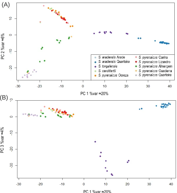
location, the number of (i) polymorphic sites; (ii) monomorphic sites; (iii) sites with data for only one individual; (iv) private sites, i.e. sites that are polymorphic in one population but monomorphic on the others; (v) sites with fixed differences, i.e. all individuals in one population are homozygotes for one allele in that site but all individuals from the other populations are homozygotes for the other allele. To evaluate the levels of genetic diversity in each sampling location, the mean expected and observed heterozygosity were calculated. Moreover, to quantify the levels of differentiation between locations, we calculated the pairwise FST using the Hudson estimator (Hudson et al. 1992). Given that the sampling locations may not correspond to populations, we investigated fine population structure with individual-based methods. To understand how individuals cluster, we conducted a principal component analysis (PCA). The number of significant principal components was determined with the Tracy-Widom test (Patterson et al. 2006) on all eigenvalues. Furthermore, individual ancestry proportions were estimated with the sparse Non-negative Matrix Factorization method (sNMF) (Frichot et al. 2014). This method infers the best number (K) of ancestral populations to explain the data, as well as the proportion of each individual’s genome assigned to each of K “populations” (ancestry proportions) (Frichot et al. 2014). We tested values of K between 1 and 10, performing 100 repetitions for each K value. We then calculated the mean expected and observed heterozygosity for each of the identified clusters, as well as the pairwise FST between them, in the same manner as before. All calculations were performed in RStudio version 1.1.383 and R version 3.4.4 using custom scripts, and the PCA and sNMF were done using the package LEA (Frichot and François 2015).

Inference of a population and species tree

Given that our sampling included different species and populations within species, we used the SNP data to reconstruct a species and population tree describing the relationships between the populations using TreeMix (Pickrell and Pritchard 2012). This program implements a maximum likelihood method and models the changes in allele frequencies due to genetic drift with a Gaussian approximation. Assuming that all sites are independent, it allows to infer the topology of the relationships among populations as the graph that best fits the variance and covariance of allelic frequencies among populations (Pickrell and Pritchard 2012). We explored a scenario with no migration, as well as models allowing for up to two migration events. Since we do not have an outgroup, the position of the root was not specified, and thus the resulting trees are unrooted.

Effect of linked SNPs

It is noteworthy that PCA, sNMF and TreeMix methods assume that SNPs are independent, and thus results can be affected by linked SNPs. Here, given the absence of a reference genome, we lack information on the location of the SNP markers. It is thus difficult to evaluate linkage disequilibrium (LD) patterns and detect linked SNPs, except for sites within the same scaffold of the catalogue. To verify if the results were influenced by potential linkage of SNP markers, we produced a dataset by dividing the catalogue into blocks of 200 base pairs and selecting only one SNP per block. For each block we selected the SNP with the less missing data. Using this single SNP dataset, we repeated the PCA, sNMF (Frichot et al. 2014) and TreeMix (Pickrell and Pritchard 2012) analysis.

Detection of introgression between S. carolitertii and S. pyrenaicus

To test for possible past introgression between S. carolitertii and S. pyrenaicus in the northern area of S. pyrenaicus distribution, we used the D-statistic (Durand et al. 2011), also known as ABBA/BABA test. This test distinguishes ancestral polymorphism from gene flow by looking at

(19)

incongruences between the gene trees and the species/population tree. To implement this test, it is required to have data from four different populations related through a fixed species tree: two sister populations (P1 and P2), a third population that could be the source of introgressed genes (P3) and has a common ancestor to P1 and P2, and one outgroup (Pout). If we define the ancestral state in the outgroup as A and the derived state in the third population as B and focus on the SNPs where the two sister populations have different alleles, there are only two possibilities: ABBA or BABA, where the order of the alleles refers to the population order (P1, P2, P3, Pout). These correspond to sites where there is an incongruence between the gene trees and the population/species tree. If ancestral polymorphism is the cause of the incongruences (i.e. no introgression), we expect P3 to be equally distant from P1 and P2 and thus the number of SNPs with the ABBA and BABA pattern to be identical. This is expected because if the two alleles were already present in the ancestral of the three populations (P1, P2 and P3) then both P1 and P2 are equally likely to share the derived allele with P3. In this case of ancestral polymorphism (incomplete lineage sorting) the value of the D-statistic will be zero. On the other hand, if there is introgression (gene flow) between one of the sister populations (P1 and P2) and the third population Figure 2.2 – Different species trees explored with D-statistic. For each species tree considered, the value of D was calculated for all possible combinations of populations, which are indicated below each population P1, P2, P3 and Pout.

S. carolitertii S. carolitertii

(20)

(P3), we expect an excess of SNPs with the ABBA or BABA pattern and D will be significantly different from zero. In that case, if there is an excess of SNPs with the ABBA pattern and a significant positive D-statistic, it indicates gene flow between P2 and P3. Otherwise, if there is an excess of SNPs with the BABA patterns and a significant negative D-statistic, it indicates gene flow between P1 and P3.

Here, we explored four different possible species trees to perform different tests, as shown in Figure 2.2. In A, we tested for introgression between S. carolitertii (P3) and two sister populations (P1 and P2) from S. pyrenaicus, one from the northern and another from the southern part of its distribution. In B, we tested if S. pyrenaicus populations from the south (P3) are more closely related to S. carolitertii (P1) or populations from the northern part of S. pyrenaicus distribution (P2). Considering the possibility of a geographical cline in admixture proportions between S. carolitertii and S. pyrenaicus in the northern part of S. pyrenaicus distribution, we also tested if the northern most sampling site of S. pyrenaicus (Ocreza – see Figure 1.1) showed more signs of introgression with S. carolitertii than the other northern S. pyrenaicus, which corresponds to scenario C. The opposite (all northern S. pyrenaicus as sister populations and S. carolitertii as the potential source of introgressed genes) corresponds to scenario D. In all cases, the outgroup (Pout) was either S. torgalensis or S. aradensis. All possible combinations of the populations shown in the figure were tested. S. pyrenaicus Guadiana was deliberately left out as there are only two individuals form this sampling location and one of them has a very high percentage of missing data (see results). Significance of D-statistic values was assessed using a jackknife approach, dividing the dataset into 25 blocks and converting z-scores into p-values assuming a standard normal distribution (p<0.01).

If introgression between populations occurred in the relatively recent past, we would expect individuals within the same population to show different degrees of introgression. To test this hypothesis, we calculated the D-statistic per individual of P2 for the same scenarios (Fig. 2.2). All possible combinations were tested, and significance of D was assessed using the jacknife approach as described above.

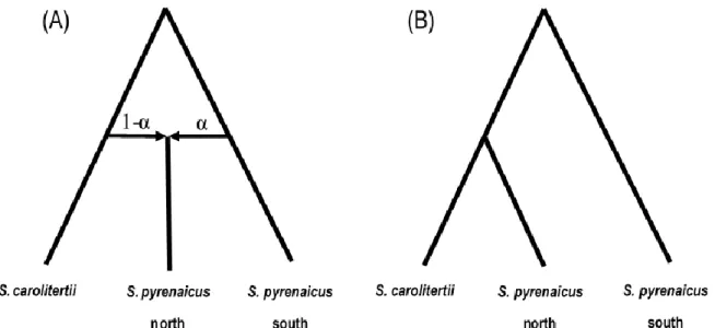
Demographic modelling of the divergence of S. carolitertii and S. pyrenaicus

We compared alternative divergence scenarios of the northern S. pyrenaicus from S. carolitertii and the southern S. pyrenaicus to test and quantify past introgression events. We used the composite likelihood method based on the joint site frequency spectrum (SFS) implemented in fastsimcoal2 (Excoffier et al. 2013). We compared the fit of two models to the observed SFS: no admixture and admixture (Figure 2.3). The admixture model assumes that the northern S. pyrenaicus received a contribution alpha (α) from the southern S. pyrenaicus and 1-alpha (1-α) from S. carolitertii at the time of the split. Note that the estimates of alpha not only indicate the most likely species tree but also quantify the level of introgression. If alpha=0 then the northern S. pyrenaicus is more closely related to S. carolitertii, whereas if alpha=1 then the northern and southern S. pyrenaicus are closer to each other. Values of alpha in between 0 and 1 indicate that the northern S. pyrenaicus received a contribution from both species, and hence indicate introgression. To test if a model with admixture fits better the observed data, we compared the likelihood of this admixture model to a model without admixture, i.e. with alpha=0. To be able to compare the likelihood values directly, models need to have the same number of parameters. Thus, in the model without admixture we allowed for a bottleneck associated with the split of the northern S. pyrenaicus from S. carolitertii, mimicking a founder effect. All parameters were scaled in relation to a reference effective size, which was arbitrarily set to be the Ne of S. carolitertii. To obtain an observed SFS without missing data, we built the joint 3D-SFS by sampling 4 individuals from S.

(21)

carolitertii and the southern S. pyrenaicus, and 6 individuals from the northern S. pyrenaicus. Given the lack of an outgroup, we could not identify the ancestral state of alleles, and hence used the minor allele frequency spectrum. To sample individuals without missing data, we used the initial dataset but without the MAF filter, and each scaffold was divided into blocks of 200bp (which is larger than the average length of the GBS loci), and for each block we sampled the individuals from each population with less missing data keeping only the sites with data across all individuals. Given that the SFS is affected by the depth of coverage, only genotypes with DP>10 were used (Nielsen et al. 2011). This resulted in an observed SFS with 8900 SNPs. For each model we performed 50 independent runs with 50 cycles, approximating the SFS with 100,000 coalescent simulations.

Figure 2.3 – Schematic representation of the two models compared with fastsimcoal2. (A) admixture; (B) no admixture. To compare directly the log10(likelihood), both models have the same number of parameters. The admixture model assumes that at the time of divergence the northern S. pyrenaicus received a contribution α from the southern S. pyrenaicus and a contribution 1-α from S. carolitertii. The model with no admixture has α=0, but to have the same number of parameters we allowed for a bottleneck associated with the divergence of S. pyrenaicus, mimicking a founder effect.

(22)

3. Results

Obtention of a high-quality SNP dataset

After the initial processing of the reads, removing low quality reads and trimming all reads to 82 base pairs, we obtained a mean of 5,223,433 high quality reads per individual. These reads were used to construct the denovo assembly catalogue. Regarding the selection of the parameters for the construction of the catalogue, we found an overall increase in the number of SNPs when allowing for higher number of mismatches, both within the same individual (M parameter) and between individuals (n parameter) (Supplementary Figures S1 and S2). When keeping the other parameters fixed, increasing the maximum number of differences between reads within the same individual (M) led to a slight increase in the number of SNPs for M between 2 and 8 (Supplementary Figure S1). When varying the maximum number of differences between reads from different individuals (n), the number of SNPs increased from n=1 to n=10, but the increment became smaller as n values increased (Supplementary Figure S2). We followed the recommendation of Paris et al. 2017 of keeping the value of n between M-1 and M+M-1 and chose a conservative value of M=4 and n=4 to create the final catalogue. This was done to maximize the number of SNPs, while minimizing the probability of wrongly treating different alleles from the same locus as different loci, and of wrongly treating similar or paralogous genomic regions as a single locus. After mapping all the reads from each individual to the catalogue, the median depth of coverage per sample was 37.5x. We note, however, that there was a large variation in the depth of coverage (DP) across individuals (Supplementary Table S2). In general, S. aradensis samples, as well as S. pyrenaicus from Quarteira, exhibited lower median DP than the majority of the individuals in the other samples.

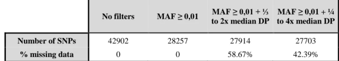
Table 3.1 – Number of SNPs and percentage of missing data for the different filtering options.

No filters MAF ≥ 0,01 MAF ≥ 0,01 + ⅓

to 2x median DP

MAF ≥ 0,01 + ¼ to 4x median DP

Number of SNPs 42902 28257 27914 27703

% missing data 0 0 58.67% 42.39%

After obtaining a dataset of SNPs found in all sampling locations in at least 50% of the individuals in each location, we applied a filter on the minor allele frequency (MAF) and depth of coverage (DP). Table 3.1 shows the effect of the different filtering options on the number of SNPs and the resulting overall percentage of missing data (per individual and per site). Prior to the application of any filters, we obtained a total of 42,902 SNPs. Applying a filter on minor allele frequency, keeping only sites with MAF ≥ 0.01, decreased the number of SNPs to 28,257, suggesting that many SNPs contained rare alleles that can be due to sequencing errors. Further application of filters on DP had a much smaller effect on the number of SNPs, only decreasing by 343 (⅓ to 2x individual median DP) or 554 SNPs (¼ to 4x DP median DP) the size of the dataset. However, these DP filters had an effect on the percentage of missing data, producing datasets with ≈59% and ≈42% of missing data respectively.

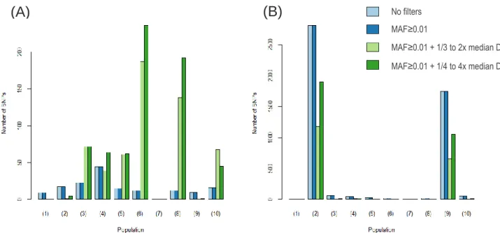
For each sampling location, we assessed the number of SNPs that significantly deviate from Hardy-Weinberg equilibrium (p<0.05) with the different filtering options, both for deficit (Figure 3.1 A) and excess of heterozygotes (Figure 3.1 B). The precise values can be consulted on Supplementary Table S3. Overall, few SNPs deviate significantly from Hardy-Weinberg equilibrium in each sampling site. These deviations can be due to artefacts, such as sequencing errors (e.g allele dropout leading to

(23)

homozygote excess) and mapping errors (e.g. mapping duplications to the same location resulting in excess of heterozygotes), or biological factors, such as inbreeding, population structure or natural selection. Even using a conservative significance level of 0.05, without correcting for multiple tests, the number of SNPs that shows a significant deviation is particularly small when compared to the total number of SNPs on the dataset (Table 3.1), indicating that most sites are at Hardy-Weinberg equilibrium and that there is no evidence for genome-wide effects of inbreeding and population structure within each sampling site. Appling filters based on MAF does not remove any SNPs significantly out of Hardy-Weinberg equilibrium (Figure 3.1), although it decreased the size of the dataset (Table 3.1). As expected if regions with very high depth of coverage were in part due to mapping errors, resulting in wrongly calls of heterozygote genotypes, the filters applied on DP decreased the number of SNPs with a significant excess of heterozygote individuals (Figure 3.1 B). It is noteworthy that the sampling location of Quarteira clearly stands out, as both species sampled in that location exhibit the highest number of SNPs with an excess of heterozygotes and that number is clearly much higher than in any other sampling location.

Considering the above results on the effects of different filters, for further analysis we decided to use the dataset filtered with MAF≥0.01 together with a filter on DP, keeping only genotypes with ¼ to 4x the individual median DP. We chose this option as it produced a dataset with lower missing data, while removing rare alleles that are likely sequencing errors (MAF filter) and discarding sites with very low quality (low DP) or that are result of mapping errors (very high DP), accounting for variation in depth of coverage per individual.

In the final dataset (filtered with MAF≥0.01 + ¼ to 4x the individual DP median), eighteen individuals have more than 50% of missing data (Supplementary Table S4). Of those, only six of them have a percentage of missing data higher than 60% but no individuals had more than 70% missing data. These individuals were distributed across sampling locations, rather than clustered in a single location. Given that individuals with a very high percentage of missing data were, at most, one per sampling site, Figure 3.1 - Number of SNPs per sampling location that significantly deviate from Hardy-Weinberg equilibrium (p<0.05) due to a deficit (A) or excess (B) of heterozygotes for the different filtering options. Each sampling location is coded by a number: (1)

S. aradensis Arade; (2) S. aradensis Quarteira; (3) S. carolitertii; (4) S. pyrenaicus Almargem; (5) S. pyrenaicus Canha; (6) S. pyrenaicus Lizandro; (7) S. pyrenaicus Guadiana; (8) S. pyrenaicus Ocreza; (9) S. pyrenaicus Quarteira; (10) S. torgalensis.

(A)

(B)

No filters

MAF≥0.01 + 1/4 to 4x median DP MAF≥0.01

(24)

with the exception of Almargem where there where two, we decided to keep all individuals in the final dataset.

Characterization of the global patterns of genetic diversity and differentiation

Although sampling locations might not correspond to populations, we quantified the genetic diversity patterns at each location. The number of SNP sites across sampling location showed two dif-ferent patterns (Supplementary Table S5). Both species sampled in Quarteira, as well as S. aradensis Arade and S. pyrenaicus Guadiana, show the highest missing data (highest number of sites without data) but also the highest number of fixed differences. The remaining sampling locations have more SNPs (i.e. lower missing data) but less fixed differences and more monomorphic sites (Supplementary Table S5).

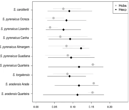
The mean observed and expected heterozygosity were similar across different sampling loca-tions, with a large variation in the expected heterozygosity distribution across sites (Figure 3.2 and Sup-plementary Tables S6 and S7). Nevertheless, the two species sampled in Quarteira, as well as S. araden-sis Arade show the highest levels of genetic diversity, with higher values of mean expected heterozy-gosity (Figure 3.2 and Supplementary Table S6). Within S. pyrenaicus, the south (Almargem, Guadiana, Quarteira) seems to harbour more genetic diversity than the north (Ocreza, Lizandro, Canha), as popu-lations in the north have lower expected heterozygosity.

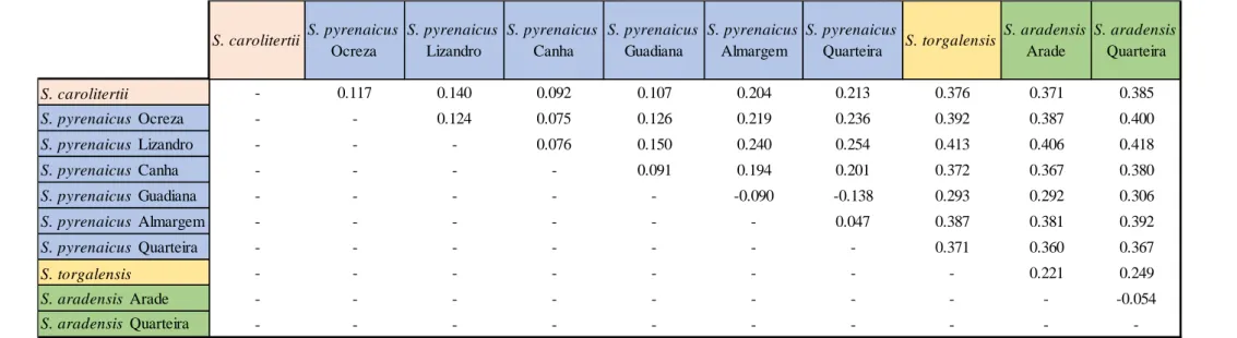
The pairwise FST estimates of genetic differentiation between sampling locations are shown in Table 3.2. The two southwestern species (S. aradensis and S. torgalensis) are less differentiated from each other than from S. carolitertii and S. pyrenaicus. Moreover, both south-western species are as dif-ferentiated from S. carolitertii as they are from S. pyrenaicus (Table 3.2). Interestingly, they are most

Figure 2.2 – Mean expected and observed heterozygosity for each sampling location. The lines represent the variation from quantile 5% to quantile 95% of the distribution across sites. Black diamonds represent the expected and grey circles the observed heterozygosity.

S. torgalensis S. pyrenaicus Quarteira S. pyrenaicus Ocreza S. pyrenaicus Guadiana S. pyrenaicus Lizandro S. pyrenaicus Canha S. pyrenaicus Almargem S. carolitertii S. aradensis Quarteira S. aradensis Arade

(25)

Table 3.2 – FST calculated between the different sampling locations. Colours correspond to those of the species distribution on Figure 1.1.

differentiated from S. pyrenaicus Lizandro (FST>0.4). For S. aradensis, there is no sign of genetic differentiation between the two sampling locations of this species (Arade and Quarteira). For that reason, they show similar levels of differentiation to all the other sampling locations, although the FST values for S. aradensis Quarteira are systematically higher (Table 3.2). Concerning S. carolitertii and S. pyrenaicus, these species are more differentiated from S. aradensis and S. torgalensis than from each other. However, it is evident that S. carolitertii is not equally differentiated from all S. pyrenaicus populations. Indeed, the levels of differentiation between S. carolitertii and northern S. pyrenaicus (Ocreza, Lizandro, Canha) are lower (FST<0.140) than between S. carolitetii and S. pyrenaicus from the south (Almargem, Quarteira) (FST>0.20) (Table 3.2). Interestingly, among the northern S. pyrenaicus sampling locations, S. carolitertii is more differentiated from Lizandro (Table 3.2). Within S. pyrenaicus, the northern sampling locations (Ocreza, Lizandro, Canha) appear to be more differentiated from the other S. pyrenaicus in the south (Almargem and Quarteira) (FST>0.194) than they are from S. carolitertii (FST<0.14) (Table 3.2). Among the southern S. pyrenaicus sampling locations, Guadiana clearly stands out as an outlier. Although it does not show any differentiation from the other southern S. pyrenaicus (Almargem and Quarteira), the FST values indicate is it more differentiated from the northern S. pyrenaicus from Lizandro and Ocreza than it is from S. carolitertii (Table 3.2). However, this result might be a consequence of the fact there are only two individuals sampled in Guadiana and one of them has a very high percentage of missing data (≈69.27%).

S. carolitertii - 0.117 0.140 0.092 0.107 0.204 0.213 0.376 0.371 0.385 S. pyrenaicus Ocreza - - 0.124 0.075 0.126 0.219 0.236 0.392 0.387 0.400 S. pyrenaicus Lizandro - - - 0.076 0.150 0.240 0.254 0.413 0.406 0.418 S. pyrenaicus Canha - - - - 0.091 0.194 0.201 0.372 0.367 0.380 S. pyrenaicus Guadiana - - - -0.090 -0.138 0.293 0.292 0.306 S. pyrenaicus Almargem - - - 0.047 0.387 0.381 0.392 S. pyrenaicus Quarteira - - - 0.371 0.360 0.367 S. torgalensis - - - 0.221 0.249 S. aradensis Arade - - - -0.054 S. aradensis Quarteira - - - -S. pyrenaicus Quarteira S. torgalensis S. aradensis Arade S. aradensis Quarteira S. carolitertii S. pyrenaicus Ocreza S. pyrenaicus Lizandro S. pyrenaicus Canha S. pyrenaicus Guadiana S. pyrenaicus Almargem