China's Impact on the Price of Oil: An Analysis in Consideration of the New Normals

(1)

China´s Impact on the Price of Oil:

An analysis in consideration of the New Normals

Thesis of Charlotte Hoefner

Master in Finance

Advisor: Professor Júlio Fernando Seara Sequeira da Mota Lobão

Faculdade de Economía da Universidade do Porto

2016

(2)

Biographical Introduction

Charlotte Hoefner was born and raised in Germany. At the age of 16 she moved to Toronto, Canada, to attend the all-girls high school Branksome Hall. Over the two-year stay in the boarding school, she was the solely recipient of the school´s scholarship for academic excellence. In 2010, Charlotte graduated with High Honors in higher levels Mathematics, History and English. She proceeded her studies in Economics at the Free University of Berlin. During her studies, she concentrated on quantitative methods, which she later applied in her Bachelor thesis on foreign exchange forecasting techniques. In 2013, she graduated from the re-known university which has been awarded with the excellence certification by the German government. After travelling through North America, she spent the first half of 2014 employed in an internship at the Corporate and Investment Bank Société Généralé in Frankfurt. The internship followed many professional experiences made during her academic studies, which concentrated on financial markets and included HSBC Trinkaus & Burkhardt in Düsseldorf (2010), Conpair AG in Essen (2011), Warburg & CO in Hamburg (2012) and Bayern LB´s ThyssenKrupp Office in Essen (2013).

Her positive experience and passion for the financial markets led her to start her Master in Finance at the University of Porto in 2014. During her stay in Portugal, she integrated quickly, while learning Portuguese and actively participating at the University´s student organization FEP Finance Club. She held the position of the Director of Financial Markets and was leading the External Relations Department from 2015 to 2016. Charlotte highly contributed to the involvement and recognition of the Finance Club, in which she led a team of more than 30 members. Her expected graduation will be in the summer of 2016, after which Charlotte is moving to London to start her professional career in the Commodities Team of Global Markets at BNP Paribas.

(3)

Acknowledgements

My sincere thanks go to my supervisor Professor Júlio Lobão who patiently and understandingly guided me in the process of the thesis.

I also thank my good friends and family, who have continuously and unlimited showed me their love and support, no matter the hour or distance.

(4)

Abstract

The qualitative research of this paper covers the most recent structural changes in the oil market and the Chinese economy. Its econometric analysis, based on a structural dynamic linear regression model, shows Chinese GDP growth rates, the Shanghai Stock Index and the CNY/USD exchange rate to have a significant impact on the monthly spot price of Brent Crude oil and improve the explanatory value of the base specification including US and China´s crude oil imports and the historic prices of Brent Crude for the time period of 2000 to 2015. A structural break of the model is found to be significant in December 2008. The consideration of the structural specific variables Chinese industrial production, urban investments and energy intensity enhance the explanatory value of the model for the sub-samples 2000-2008 and 2009-2015 further. Its consideration of time lags and critical consideration of data allows for the confirmation of the observed fundamental changes in the oil market and China´s economy, which are change in the price elasticity of demand and supply, the strategic reserves of crude oil in China and the plateau of oil demand growth for urban areas. The analysis further finds, that the consideration of geopolitical events as dummy variables is not significant in most cases. The analysis confirms the observation by some studies, that China´s imports have no significant impact on oil prices, but found other explanatory variables to be significant. This result stresses the importance of an economic analysis to allow for a careful consideration of data and the awareness of their limitations.

(5)

Tables

Table 1: Methodology ... 20

Table 2: Descriptive Statistics Main Variables, 2000-2015 ... 22

Table 3: Regression Results Specification 1 ... 25

Table 4: Explanatory Value of Specification 2 ... 28

Table 5: Regression Results Specification 3 ... 29

Table 6: Vector Inflation Factors Specification 2 ... 41

Table 7: Test Statistics Specification 2, 2000 - 2015 ... 42

Table 8: Vector Inflation Factors Specification 3, 2000 - 2015 ... 43

Figures

! Figure 1: Crude Oil Price Evolution, 1970 - 2015 ... 4

Figure 2: Shanghai Composite Index, 2014-2016 ... 8

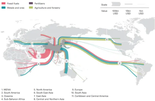
Figure 3: Resource Flows into China, 2014 ... 34

Figure 4: History of Internationalization efforts of the Yuan, 1994-2016 ... 35

Figure 5: China´s largest oil fields ... 36 !

(8)

0.! Introduction

In 2008, the international oil markets were strongly affected by the financial crisis. As the world economy only slowly recovered, oil prices did not reach the same price levels as before the crisis. Instead, oil prices fell to less than 30 USD/Barrel in 2016. This development was highly and controversially discussed in the media and eventually academic researchers joined the discussion. The main focus was to determine whether the decrease in prices was supply or demand driven, similar to the prior discussion on the rise of oil from 2000 to 2008. But different to the previous decade, the supply side as well as the demand side had undergone fundamental changes. The additional shale oil resources have restricted the, once dominant, power of the Organization of the Petroleum Exporting Countries (OPEC) and undermined the notion of imminent oil resource scarcity. On the demand side, it has triggered China to become the most important market for crude oil imports. Meanwhile, the growing dependency of China in the past decade has increased the concerns by Chinese authorities on energy security. In response and supported by the recent slowdown of economic growth, Chinese authorities changed their economic strategy from quantitative to qualitative growth targets. The new policies concentrate on less energy dependency as well as social stability within the country. Concerns on sustainable economic growth is addressed, while the Communist party is concerned to remain its legitimacy for power.

Both developments have been described with the term “New Normal” as the changes are considered structural and permanent. Although, this opinion seems to be shared by market observers as well as academic researchers, little literature has captured this change. The hypothesis of changing regimes, resulting in structural breaks, has been extensively discussed, however, often concentrating on geopolitical events, financial speculation and the financial crisis of 2008. Little quantitative academic research can be found on the “New Normals” in the oil market and the Chinese economy, whereas numerous business reports and articles have covered the matter.

This study fills the gap in existing academic literature and concentrates its evaluation on the observed structural changes in the oil markets and China´s economy. It successfully uses a dynamic multiple linear regression model to support arguments in favour of a structural break in 2008. Further, by doing so, it enables to observe changes in the

(9)

importance of fundamental variables driving the market. More than the majority of the observed results considering significance level of past Brent Crude oil prices, US and Chinese oil imports, Chinese GDP growth, CNY/USD exchange rates, Shanghai Stock Index level, urban investments, energy intensity levels and the industrial production index support the qualitative observations of changes in the international oil market and China´s economy specifically. It is found, that a detailed specification of the model, considering economical and structural changes in China, describes better the price changes of Brent Crude in the sub-sample periods of 2000 to 2008 and 2009 to 2015 than the base model, which only considers historic Brent crude prices and imports. The consideration of economic variables further enhances the explanatory value over the entire period in comparison to the base specification. Previous studies (Mu and Ye 2011) have neglected such an extensive analysis, and restricted their study on imports which showed to be non-significant. Therefore, this paper considerably adds to existing literature, as it critically assesses whether China´s imports are the best measurement of its impact on oil prices.

The most important conclusion of this research is therefore, more than the specific regression results, that a detailed analysis of the oil market and China leads to a better understanding of econometric results and inherent data limitations. This is of high importance as changing oil prices have a large impact on oil importing as well as oil exporting countries. A close relationship between economic growth and oil prices has been agreed on and, after all, recent deflationary pressure has also been attributed to low oil prices. The effects on economic performance by the oil price are therefore apparent and observable. A better understanding of the fundamentals, that are driving the oil prices, supports the finding of reasonable economic targets as well as effective economic and energy policies.

This paper will proceed by presenting the qualitative analysis of the changes in the international oil market and the Chinese economy. It is followed by an overview of academic literature on international oil prices, economic and oil price relationships and the China Factor. The review includes a discussion of econometric techniques. In the third chapter, the method and data of the research is presented. It is followed by a discussion of the results and the conclusion.

(10)

1.! The Time of New Normals

Since the financial crisis, important changes have taken place in the global oil market and in the Chinese economy. The shale oil revolution changed the dynamics of the international oil market. Meanwhile, China has targeted qualitative economic growth after economic growth rates were disappointing and concerns on the health of its economy were rising.

This chapter will provide the most important insights into the two markets. The changes observed in this context will argue in favour of new fundamentals driving the crude oil price. The analysis will provide a set of variables that are expected to contribute to the estimation of the impact on international oil prices by China´s oil demand and be used considered in the econometric analysis of this paper.

1.1. The New Normal in the Global Oil Markets – The Effects of the Shale Oil Revolution

The most recent decline in oil prices, starting in 2014, has caused many to reconsider the classical assumptions on the economics of oil. Today, it seems clear that the decline was caused by an unexpected increase in conventional oil (non-US production) and a decline in world economic growth (Badel and McGillicuddy 2015, Baumeister and Kilian 2015). The reason for why the market was not affected by prior decreases in conventional oil supply can be found in the shale oil revolution which started in 2009. The created additional shale oil output from the US did not disrupt the oil price and did not create a downward pressure on prices as it might be expected by economic theory, ceteris paribus. Instead, the additional output added to the stability of oil prices, as supply from traditional oil producers, such as Libya, was disrupted (Mănescu and Nuño 2015).

(11)

Figure 1: Crude Oil Price Evolution, 1970 - 2015

Source: Energy Information Administration (2015)

Figure 1 shows the evolution of the West Texas Intermediate (WTI) spot price and the acquisition cost of crude oil prior to 1986. Current oil price levels below 50 US-Dollar per Barrel (USD/barrel) are very low compared to the last decade, but oil prices have been at much lower levels in historical comparison (for examples prior to 2000 and prior to 1975).

The fast expansion of shale oil rigs in the US was supported by country specific advantages. After all, shale oil extraction is derived from shale gas extraction combining hydraulic fracturing with horizontal drilling. The procedure is, therefore, based on well-known principles and shale oil resources can be found numerously in other countries, with Russia holding the largest resources of shale oil reserves worldwide. But the US had the experience of extracting shale gas, legal incentives for landowners, including private ownership rights, existing infrastructure of pipelines that support the distribution of oil and easy access to global capital market funding (Mănescu and Nuño 2015). These advantages combined with high oil prices motivated the shale oil to take place in the US.

As a result, the US transformed from an oil importing country to a net oil exporting country and is expected to become energy self-sufficient by 2030. Whereas the shale oil rig count in the US has been rising until 2014, it began to decline once prices started to decrease in 2014. Even though break-even prices for shale oil extraction range from 30 USD/barrel to 100 USD/barrel, market observers estimate the average break even price to be at 50 USD/barrel (Rapier 2016). Once prices decreased in 2014, OPEC and especially Saudi Arabia was expected to cut production. However, they surprised markets

(12)

when they did not do so and instead maintained production levels to force high-cost oil producers out of the market, including shale oil producers. The downward price trend continued and at the end of 2014 and a decline in US shale oil rigs was observed. Additional investments into the shale oil industry stayed absent causing maturing rigs not to be replaced. The short life-cycle of shale oil rigs contributed to this development. By 2016, the market observed a second development: debtor-in-possession financing allowed shale oil companies, who had filed for bankruptcy, to continue production and even invest in the productivity of existing rigs1. The strategy by shale oil producer was to stay in the market, until prices would increase again to the critical value of 50 USD/barrel (as they did in May 2016).

As soon as the critical price of 50 USD/barrel is reached, the market expects shale oil production to increase again2. This behaviour of shale oil producers defines them as swing producers and limits the price range of oil considerably (given constant demand). The previous market power of OPEC over oil price levels is hence restricted to levels below 50 USD/barrels and bears considerably high opportunity costs (Mănescu and Nuño 2015). Alternatively, the shale oil market could continue to evolve and enhance its technology to decrease production costs further, and become more competitive3_{at prices below 50} USD/barrel, further restricting OPECs market power.

The emergence of shale oil production has hence not only changed the role of the US in world oil markets, but also decreased the market power of OPEC. Furthermore, traditional theorems considering oil as a scarce resource and discussion on peak oil production have been muted to wide extent. Additionally, it is unlikely, that the market will evolve backwards, as shale reserves in China and Argentina are expected to be developed once the required infrastructure is developed. Therefore, the development can be considered of structural and sustainable nature, characterizing the shale oil revolution to have caused new market principles referred to new economics of oil.

#

########################################################

1_{See the articles by the market observers Rapier (2016) and Gopinath and Schneyer (2016) for a detailed}

discussion of the matter.

2_{Uncompleted wells, which are referred to as “fracklog”, can quickly start production within six months,}

requiring lower capital investments than conventional crude oil rivals.

(13)

1.2. China´s Economic Development – A Path towards Qualitative Growth

The shale oil revolution might have just occurred at the right time. Due to the extensive growth of China´s economy, China´s demand for energy and specifically oil increased in the short run (Yuan et al. 2008) and long run (Zou and Chau 2006). As China transformed from an oil net-exporter into a net-importer in 1993, it had to consider new sources for crude oil. Oil sources came primarily from trading partners in the Middle East and Africa4, sometimes competing for resource with the US or undermining international embargoes set by the US (Shinn 2010). Zweig (2005) underlined the growing tension, caused by the competition for future oil reserves and international secure transportation of oil. Referring to the power transition theorem5, if not carefully managed, such a challenge to the power of the US could have resulted in severe suffering of international relations. To a great extent, the shale oil revolution hence eased the tensions over future oil reserves.

China has experienced an average economic growth rate of 10% between 2000 and 2011. The growing industry was motorized by the country´s industrialization. The growth resulted in rising demand for commodities, including oil. Since 2014, GDP growth rates have been disappointing market expectations and have, therefore, been observed closely by market participants. For the first time in 2012, the Chinese economy did not meet its target growth rate, when industrial production and exports started to decrease. Until the end of 2015, quarterly year-on-year (yoy) growth had slowed down to 6.8% in the last quarter.

The slowdown in economic growth reflects different economic developments and has been interpreted as the consequence of past political market interventions. As much as they are currently discussed in media, they were observable already in the aftermath of the financial crisis. Morrison (2009) reasons uneven economic growth and a high dependency on foreign trade to have made China subject to the financial crisis in 2008 in the first place. The importance of exports had previously motivated Chinese authorities to peg the Chinese Yuan (CNY) against the US Dollar until 2006. Eventually, the peg was restored after the financial crisis and, although, the Chinese government stressed

########################################################

4 _{The international trade flows of commodities to China are illustrated in Appendix 1.}

5 _{The power transition theorem states, that if the power of a nation is challenged by another nation, the}

nation in power will undermine (declare war on) the increase of the power by the challenging nation as long as it has an advantage.##

(14)

internationalization efforts, the Yuan was recently devaluated in May 2016. This is interpreted to hinder future development and to undermine past internationalization efforts, such as the addition of the CNY into the IMF reserve currencies basket6.

The pressure on the CNY increases, as the Federal Reserve Bank is planning to loosen its monetary policy further. This would force China to either spend additional foreign reserves on the devaluation of the CNY or allow the currency to appreciate. If Chinese authorities allow a free floating currency, the Yuan is expected to increase significantly, as the currency is considered to be undervalued (Balding 2015). The pessimism on the future development of the Chinese Yuan and the Chinese economy can be observed in the amount of capital outflow of the economy. The Chinese government reacted by implementing stricter capital controls and by increasing taxation on exchange transactions in 2015 and 2016. The trend of Chinese companies and households to rather invest in foreign assets reflects to a reasonable extent the distrust in future economic prospects. Eventually, any actions by the Chinese government to limit capital outflows would question their economic management skills (Balding 2015).

Besides net capital outflow, the devaluation of the Yuan has contributed to the evolvement of cheap credit (Morrison 2009). This resulted in oversupply capacities and bad loans, which impose today a severe problem for the Chinese economy. Most recently, Chinese debt is rising faster than economic growth and low interest rates have been used to re-leverage non-performing loans. Especially public debt, and more specifically debt levels of state-owned enterprises (SOE), are of concern. Gracie (2011) and Morrison (2009) argue the Chinese government to be the reason for the problem: Through continuously and unrestricted support for SOE, resources are diverted away from efficiently, profitable businesses and instead unprofitable SOEs, also referred to as

Zombie Companies, are kept alive. Market observes do not agree, on whether the problem

will self-correct itself or whether the conflict between economic and political objectives can be resolved by the Chinese government (Curran 2016, Gracie 2015). Lastly, however, capital requirements for Chinese banks have been lowered and the falling real estate market raises concerns over the highly leveraged economy, drawing similarities to the real estate market crisis in the US, which resulted in the financial crisis of 2008. In May 2016, Curran (2016) reported for Bloomberg, that Chinese authorities started to allow for ########################################################

6_{An overview over internationalization efforts and time in which the CNY/USD was pegged or devalued,}

(15)

more defaults and that the Communist Party Newspapers reported China´s debt pile as the “original sin” which would not support long term economic health. This can be interpreted as a change in the government´s sentiment towards its rising debt levels and slowdown in economic growth. Alternatively, it can be interpreted that the circumstances forcing the Chinese government to act have harshened.

Meanwhile, business success in China has been traditionally tied to the relationship of business owners to the Communist Party. Corruption is an eminent problem in China and the regulatory environment is poor (Morrison 2009). Intellectual ownership rights are not well established and regulations are not transparent and found to be inconsistent. Additional to the inefficiencies created by the credit market, and decreasing economic growth, the Chinese stock market fell severely in the summer of 2015. It resulted in an additional increase of capital controls, to which the Chinese government reacted with additional government intervention in the financial markets. As Figure 4 shows, the different government interventions as well as currency policies could be observed in the Shanghai Composite Index.

Figure 2: Shanghai Composite Index, 2014-2016

Source: Curran (2016)

Most importantly, a growing economy is perceived by the Chinese government vital to secure social stability (Morrison 2009). Public unrest had been growing in 2005, when the Chinese population did not perceive to be benefitting from the rapid economic growth. Lately the income gap between the rural and urban area and environmental pollution had been of rising concern. Balding (2015) argues that the Chinese government will, therefore, more extreme than in Western countries, try to foreclose unemployment and hence mute possible protests. However, to target the economic problems and secure

(16)

economic growth stability, Balding (2015) argues, no measures would be without negative consequences for at least some part of the population. One way the government is trying to achieve this balance is by increasing energy efficiency and decreasing energy intensity. A number of reforms and measure have set in place, to transform the economy and support qualitative growth. The set of rules has been referred to as China´s structural reforms and describe the transition from a manufacturing industry to a service oriented industry.

1.3. China´s Structural Reforms – The Impact on Oil Demand

Given the strategic value of oil, the commodity has been traditionally of high concern to oil importing and exporting nations. Therefore, many oil importing countries, including China, are targeting energy security as the dependency on oil imports is perceived risky (Roncaglia 2003). Energy security can either be accomplished by ensuring sufficient resources and safe transportation from the exploration side to industries and households or by reducing energy intensity and energy efficiency. Energy intensity in any country is expected to decrease over time, assuming economies to develop into service oriented industries and technology to allow increases in energy efficiency. China has targeted both options. This chapter will therefore examine policies specifically implemented to target energy efficiency and intensity as well as structural reforms changing the energy intensity and efficiency levels.

The imports of oil have been rising since 1993, as consumption levels exceeded production levels and oil reserves in China were declining7. The reserve to production ratio for oil (number of years until traditional oil reserves deplete) was estimated to be 12 years in 2007 by Pang et al. (2009). The peak of production might be delayed when energy efficiency is increased and energy intensity is reduced. The target rate of 16% less energy consumption per unit of GDP has been announced within the 12th Five-Year Plan (2011 – 2015) by the Chinese government. This implied a shift from an economy, based on manufacturing, to a service-industry. The IEA measures oil intensity as the amount of oil products used to generate Yuan 1 Billion of GDP (IEA 2015). In 2014, the oil intensity was measured to be at 0.54 kb/d for Yuan 1 Billion of GDP. Compared to levels when China was just entering the heavy industry sector in 2004, this is a 34% decreased. The

########################################################

(17)

IEA expects the oil intensity to decrease further to 0.43 kb/d in 2020. Besides energy intensity, other key targets covered lower carbon intensity and a higher share of non-fossil energy. On the other hand, Li (2007) points out the supremacy by Western countries over Asian countries in world-oil usage and the gap between them. If China was to reach the same per capita levels as Western countries, it would translate into for higher energy consumption and hence more oil demanded.

In 2015, a cap on total energy consumption (4 billion tons of coal equivalent) in 2015 was introduced. This gives reason for the industry (IEA 2015) and academics (Meidan, Sen and Campbell 2015) to reference the set of policies and the following changes in the Chinese energy market as the “new normal”, adopting the term first used by Xi Jinping. In the 13th five-year plan (2016 – 2020), the Chinese government underlined to aim to aspire social inclusivity and environmental sustainability by decreasing manufacturing overcapacity and stimulating technological innovation. Technological innovation and private investments specifically apply to the energy sector (EIA 2015). The pricing schemes in the energy sector are increasingly determined by market forces and increased energy transmission infrastructure. Efficiency gains were recorded at 3.7% per annum between 2008 to 2014 and forecasted efficiency gains from 2015-2020 are expected to match these levels (IEA 2015).

The new strategy for economic growth concentrates on the quality of growth, accepting lower absolute economic growth rates between 6% and 7%. A sustainable growth is considered to be also socially stable and hence might diminish excessive social tensions (Roncaglia 2003). A matter, which is of constant concern for the Communist party, as its legitimacy is considered to be dependent on strong and sustained growth (Shinn 2010). Additionally, future economic growth should be driven by domestic consumption instead of net exports, investments or government spending. However, Gracie (2015) underlines that China´s demographic structure and debt problem have not been addressed to this point and that essential structural reforms have failed.

It is uncertain, whether the demand for oil by the manufacturing industry will be replaced by an other sector of the economy (Kawa 2016b). But although the times of extensive economic growth might be over, the demand for oil per person in China is still far below levels in America and Europe. Whereas China´s citizens only consume one ton oil

(18)

equivalent per year (TOE/year), levels in Europe are at four TOE/year and eight TOE/year in the US (Anandan and Ramaswamy 2015).

The demand for diesel and gasoline products is decreasingly attributed to the industry sector. The percentage of diesel demand allocated to the industry sector has almost halved in 2014, compared to levels at almost 40% in 2002. A similar trend can be observed in the demand allocation for gasoline (Meidan, Sen and Campbell 2015). Meanwhile, the allocation of demand for gasoil and diesel to transportation has been rising compared to other sectors, while the demand for motor gasoline and jet fuel is expected to continue to grow further in absolute terms as well (IEA 2015). Therefore, it is likely, that the transportations sector in China will continue to its significant contribution to oil demand growth, as it has done since 2008 (Kawa 2016a).

China´s per capita vehicle ownership is much below the per capita vehicle ownership in developed countries, although, car ownership numbers have risen in the past years. Furthermore, although the populous country provides a large potential market, its urban density is self-limiting and road infrastructure is much less developed than in the US or Europe. Past and future environmental concerns have and will result in policies impacting the use and purchase of cars (McCracken 2010). Given the development of the oil use intensity of cars, the evolvement of electric cars and the state of China´s economic development, it might not be necessary that increased car ownership increases the China´s demand for oil.

The above argumentation may mislead to the assumption, that if a growth in oil demand from the transportation sector is observed, it would reflect economic growth. However, McCracken (2010) points out that an increase in domestic car sales, must not necessarily be in line with the China´s economic development. Instead, the government subsidised car sales in rural part of China and decreased taxes on newly purchased small vehicles. Car sales further might not indicate the number of people who are actively using the vehicles. Cars have been considered a status symbol for the middle and while car sales have been declining in 2015, car registrations increased (Kawa 2015).

(19)

2.! Literature Review

The discussion in academic literature has been very controversial and not all authors agree on a demand driven oil price development, but rather consider crude oil supply changes8_, OPEC output restrictions9_{, speculative behaviour by market participants and/or financial} speculation10 and inventory levels11 as significant forces. Others have concentrated their studies on the macroeconomic affects of oil price shocks12. Given the number of research conducted, this literature review will concentrate only on a selection.

The selection will concentrate on econometric techniques used to study oil prices. The chapter will give an overview on different methods, the discussion of linearity and non-linearity between oil prices and the macro-economy and the importance of regime changes. The literature review will proceed with an overview on different results found in regards to the impact of China on the international oil prices.

2.1. Econometric Techniques

Reviewing literature on the oil price leads to the observation that studies either analyse the oil market movements and changing regimes in hindsight, or (more often) models are tested to forecast future oil prices. Generally, the benchmark crude oil prices, Brent Crude Oil or West Texas Intermediate are considered for such analysis.

Fattouh (2007) differs between non-structural models, demand supply models and informal models, and concludes none to provide sufficient forecasting power. Baumeister and Kilian (2016) argue that the reason for significant forecasting errors in the estimation of future crude oil markets might not be because of unknown determinants of the crude price, but rather because of forecasting errors in the estimation of explanatory variables. Furthermore, they observe forecasting errors to change in size depending on the nature of the demand or supply shock. Behmiri and Manso (2013) highlight that there is no consensus on which techniques are most reliable when forecasting crude oil prices. They differ between qualitative and quantitative methods. Qualitative methods would include approaches such as web text mining but are not considered in this review of existing ########################################################

8_{E.g. Gallo et al. (2010)}

9_{E.g. King, Deng and Metz (2011)}

10_{E.g. Fattouh, Kilian and Mahadeva (2012)} 11_{E.g. Bern (2011), King, Deng and Metz (2011)} 12_{E.g. Jones, Leiby and Paik (2004)}_#

(20)

literature. Rather, econometric methods are concentrated on and more precisely structural models. Structural models are divided by Behmiri and Manso (2013) into OPEC behaviour models, inventory models, combination of OPEC behaviour models and inventory models and models based on supply and demand. Although, they find only little evidence for the forecasting power of structural models, they highlight their explanatory value for past price movements.

It can be observed in previous literature, that there has been a trend from using linear models to describe the relationship between economic growth and oil prices until the mid-1980s to non-linear specifications afterwards (Ghalayini 2011). The reason for the shift in the techniques is a study by Mork (1989) that showed that the US economic activity replied asymmetrically to real oil price changes: Whereas there was a significant impact by oil price increases on the economic activity, there was no significant impact observed when the oil price was declining. More recently Krugman (2016), reporting as a market observer for the New York Times, wrote that last decline in oil price did not have expected positive effects on the economy, but rather, the marginal size of change led to negative implications for world economic growth. Therefore, the traditional relationship between oil price declines and the economy, might not hold true anymore. Krugman (2016) argues the deleveraging effect by oil producers results in negative externalities for the global economy and the change in paradigm to be caused by the short cycle investments of the shale oil industry. In literature, Hamilton (2010) observes non-linearity of larger changes in oil prices using Kilian and Vigfusson (2010) as a reference paper. Ghalayini (2011) and Hamilton (2010) agree, that the review of literature conducted on the subject provides no clear answer.

Whether linearity is found or not often depends not only on the method (Ghalayini 2011), but also on the data sets used for the model (Hamilton 2009). Cong and Wei (2008) further underline the difference effects the stage of development of a country has on the linear or non-linear relationship between crude oil prices and economic growth. As a non-linear relationship might be apparent for OECD countries and developed countries, the same might not be true for developing countries such as China. Ghalayini (2011) underlines, that although the trend is apparent in empirical literature, the same trend cannot be observed in the theoretical literature. The exception she finds is based on the dispersion hypothesis developed by Lilien (1982), which is also considered by the analysis of Cong and Wei (2008) when studying the impacts of crude oil prices on the Chinese stock

(21)

market. Lilien (1982) highlights the different effects oil crude price changes have on different sector, depending on whether they are energy efficient or energy intensive, and hence lead to readjustments across sectors which require different sets of time.

Once a relationship between economic growth and the oil prices is established, most academic papers agree that they might not be robust over time. Instead, it is usual to observe significant results for tests, that assess structural breaks in the models. Hamilton (2008) underlines that oil price changes are affected by different regimes at different times. Kilian and Hicks (2013) consider the period 2000 to 2008 without structural breaks, while Lechtahler and Leinert (2012) restrict the sample to 2003 to 2010 because of the observation of a structural break in 2003 in most time series, and criticize the results of studies not accounting for this specific break. Gallo et al. (2010) also find a structural break in March 2003 in the demand from China. They argue the Iraq war to be the reason for the structural break, while the increasing economic growth from China attributed in their opinion for the earlier structural break in their data set in 1991. Furthermore, they highlight that evidence for structural breaks differs between countries. Du, He and Wei (2010) confirm the existence of structural break in January 2002 (for the period between 1995 and 2008) and reason them with the changes in China´s oil pricing mechanism. Ji (2012) found a similar change in the impact of explanatory variables, assessing fundamental variables only to have a long run impact before the financial crisis, while short term oil price behaviour was explained by speculation. Such mechanisms were set off during the period of the financial crisis and fundamental explanatory power was re-established after the financial crisis.

2.2. The China Factor

The resulting increase in demand for crude oil from China is argued by Kilian and Hicks (2013) and Hamilton (2008) to have driven the international crude oil prices up from 2000 to 2008. Gallo et al. (2010) found the consecutive rise in oil prices from 2009 onwards caused by growing demand for oil from China. The latest decline in oil prices starting in 2014, was argued by Anandan and Ramaswamy (2015) to be due to low growth rates of China´s economy. Other, such as Bern (2011) highlights the many additional factors that determine the oil price besides supply and demand fundamentals. Explanatory variables could be expected to include stock markets and foreign exchange markets besides economic growth.

(22)

Beirne et al. (2013) analysed the China factor on the world economy through quantifying the influence of Chinese GDP growth on oil prices. Using a country-level demand model, based on 1965 to 2011, crude oil prices are estimated from 2010 to 2030. They find an increasing premium added to the price of oil by China. Kilian and Hicks (2013) stress the market´s underestimation of the respective growth rates and observe the real price of oil to react to unexpected growth in emerging in markets in a hump-shape, measured by revisions of professional GDP forecasts from 2000:12 to 2008:12. The measured surprises are observed to exist in a higher extent for Asian economies than for OECD economies13, namely from China and Russia but also for OECD country Japan. Annual revisions of Chinese economic growth rates´ estimates by 0.1 percentage points led to a five percent increase of the crude oil price. Kilian and Hicks (2013)´ findings, based on a linear regression method and historical decomposition, confirm the results by Kilian (2009), who used a structural VAR model. The observation is contradicted by Lechtahler and Leinert (2012). Lechtahler and Leinert (2012) found that demand from emerging countries (India, Russia, South Africa, Indonesia and China) did not contributed additionally to the impact of the demand from OECD countries during the increase of oil prices from 2003 to 2008. Only during the peak of the oil price in 2008, a difference in the effect of cumulative demand and OECD demand was observed. Du, He and Wei (2010) find similar results as Lechtahler and Leinert (2012) for the period from 1995 and 2008, using a multivariate vector autoregressive model. They found no oil pricing power by China on the oil market.

Kilian (2009) differs between the effect of supply and demand shocks on the oil price. On the demand side, he differs between shocks specific to crude oil and demand shocks effecting global demand for all commodities. In his analysis of the real price of oil from 1975 to 2007, he found changes in expectations result in precautionary adjustments in demand, specifically effecting crude oil and resulting in a sustainable, immediate and large change in the real price of oil. Contrary, the effects by demand shocks on all commodities appear with a time lag but are also persistent. Kilian (2009) concludes most changes in the oil price to have resulted from demand side shocks and the increase in the real price of crude oil from 2003 to 2007 to have been driven by an increase in the

########################################################

13_{The analysis concentrates only on the United States, Germany and Japan as OECD representatives, while}

(23)

aggregate demand for industrial commodities as well as specific increasing demand for crude oil.

Additional to the studies presented above, Kilian and Lee (2014), Fattouh, Kilian and Mahadeva (2012) and Smith (2009) support the impact by Chinese economic growth on the crude oil price. Mu and Ye (2011) found China´s imports not to significantly impact the oil price from 2002 to 2008 and conclude China not to have had a significant impact on the rising oil prices.

Whether the relationship between economic growth and the oil price is bilateral or unilateral is the subject of many additional studies. While some studies assume a bilateral relationship for which they make use of the vector autoregressive (forecasting) technique, other consider granger causality tests to identify the direction of a possible significant impact or calculate price elasticities. Ghalayini (2011) finds the impact of crude oil prices on economic growth to be dependent on the state of an oil net importer or oil net exporter. China, as a net importer of oil since 1993 is found to have a negative correlation between changes in oil prices and Chinese economic growth from 1986 to 2010. The economy can be affected by an oil price change through either the demand or supply side. Using the demand side channel, the disposable income of consumers is positively affected. When oil price rises, products derived from oil are expected to become more expensive and hence less income is available for other goods and services. As oil prices increase, the costs for producers using oil as an input factor increase as well and hence negatively impact investment decisions. The supply side channel considers the increase in production costs when oil is used as an input factor and hence can result in a reduction of the output by the firm.

Gallo et al. (2010) observe demand variables not to significantly impact oil prices, but changes in the oil prices to effect demand and supply variables from 1990 to 2009. Askari and Krichene (2010) find oil demand price elasticity very low and/or insignificant for the period from 1970 to 2008, confirming earlier results from Cooper (2003), who found no significant price elasticity of demand for China from 1979 to 2000. Instead Askari and Krichene (2010) found oil demand mainly responsive to income. Results by Hamilton (2008) contradict the study, when he observed that from 2002 to 2007 price elasticity of demand at lower levels than in 1980. He argues that this development is in line with the main demand for crude oil deriving from transportation which only has little substitution

(24)

possibilities, compared to different uses of oil, demanded to a higher extent before, allowing more substitutions. Bern (2011) observes that the transportation sector was inelastic to the high prices of oil in 2008 but private consumers were outweighed by industrial users of crude oil, who cut production.

Behmiri and Manso (2013) underline the use of non-oil variables such as economic activity, interest rates, exchange rates and other commodity prices in structural models (see also Bern 2011). Although they criticize the forecasting performance, they observe fundamental variables to explain price movements well. However, the complexity of structural models and data limitations restricts their use for such purposes and therefore models using time-series techniques are used more frequently. Gallo et al. (2010) describe in their review of literature, economic growth, inflation and other economic indicators to provide inconclusive evidence. Ghalayini (2011) highlights that oil prices can also have a converse indirect effect on economic growth through influencing foreign exchange markets and inflation. The findings on whether the economic growth impact the oil price, vice versa, or whether there exists a bilateral relationship are not conclusive. Ghalayini (2011) reasons the difference to appear, as different models propose different results. If an increase in economic activity would lead to higher oil prices, then the effect of higher oil prices on the economy, described by Ghalayini (2011) as feedback relationship, can mitigate the direct impact.

Askari and Krichene (2010) and highlight furthermore, that the demand for crude oil depends besides economic activity also on demographic and technological factors. Urbanism and residential expansion will impact the demand for energy. In rural areas, vehicle substitutes are limited whereas the use of vehicles in large cities is limited. Additionally, rural areas might also not be connected as much as urban areas to the energy grid in developing nations. Crompton and Wu (2004) estimated the growth of energy consumption to decline by 2010, due to structural changes in the economy. Additionally, technological factors will impact energy intensity and energy efficiency of a country and for example, the loss of energy in the refining process of oil, or energy efficiency of vehicles. Not accounting for the complexities of the supply and demand determinants will increase the costs of misspecification and omission errors for econometric models (Askari and Krichene 2010).

(25)

3.! Model and Data

This chapter explains the model used in the analysis, discusses the methodology applied as well as the choice of parameters based on the qualitative economic analysis provided in Chapter 1.

The analysis will consider the time period from 2000 to 2015. This time interval will include the industrialization of China´s economy as well as the financial crisis and the shale oil revolution. The data is limited to December 2015, as some economic indicators considered for this analysis have not been published for later period by mid-2016. Although a longer time series would increase the number of observations and hence enhance the asymptotic properties of estimators (Lechtahler and Leinert 2012), it also would lead to a higher probability of structural breaks in the time series describing the oil market. The monthly intervals are in line with most structural models reviewed by Behmiri and Manso (2013).

The explanatory variables considered in this analysis, are expected be to some extent endogenously defined. This is reasonable for the close interaction between oil prices and economies. To account for endogenous variables, co-integrated vector autoregressive (VAR) models have been applied in previous academic literature. The method is neglected for this analysis, for the same reasons as Askari and Krichene (2010). Co-integrated VAR models include the analysis of the co-integration factors of all variables which are numerous in this analysis. Furthermore, the model would have constraints in the identification of assigning values to parameters and whether their relation belongs to the vector space of co-integration vectors. Therefore, dynamic multiple regression model is estimated. The restriction on the interpretation of its coefficients is out-weighted by the possibility to consider different variables for the analysis of China´s impact on the oil price. The relationship between the economic indicators and the oil price is considered to be linear for developing countries (Cong and Wei 2008). China is categorized as a developing country, based on the low per capita levels of the economic indicators in international comparison (Li 2007).

(26)

3.1. Model

#

The oil price is assumed to be based on supply and demand, which through market clearing fulfils an equilibrium condition in each month. In equilibrium the quantity demanded (QD) is equal to the quantity supplied (Qs), equation 1.0.

QD = QS (1.0)

QS = cS + βSP pt + βS(j) pt-j + uS,t j= 1,2, …, 12

(2.0)

QD = cD + βDChina QDchina, t + βDChina(i) QDChina, t-I + βDC QDC, t + βDC (i) QDC, t-I + βDChinaIV pt QDChina, t + βIVChina(i) pt-i QDChina, t-i + βDUS QDUS, t + βDUS(i) QDUS, t-i + βIVDUS pt QDUS, t + βIVDUS(i) pt-i QDUS,

t-i + uD,t i= 1, …, 6

(3.0)

The world aggregate supplied (2.0) is defined by a dynamic model, assuming production to be supplied by residual producers whose price setting decision is simulated recursively by current and past oil prices (Stevens 1995). The quantity demanded (3.0) is dynamically modelled by considering the demand from China (QDChina) and the US (QDUS)), who are

the biggest consumers of energy and the biggest importers of crude oil in the time period from 2000 to 2015. The different economic structures lead to different impacts on oil demand in response to changes in the oil price (Askari and Krichene 2010). The difference is accounted for through interaction variables (pt QDChina and pt QDUS).. In

addition, explanatory variables can be included to describe the Chinese economic development and structural changes more accurately, which will take the place of QDC.

The intuition for equation 2.0 and equation 3.0 is described in more detail in Appendix 4. The equations presented above are simultaneously solved for pt , which results after simplification of the coefficient representation in equation 4.014.

pt = cp +bQDchina, t + b (1+i) QDChina, t-I + γt + γt-i + bIV, China) pt-i

QDChina, t-i + bUS QDUS, t

+ bUS, (1+i) pt-j QDUS, t-j +βIVDUS(i) pt-i QDUS, t-i – bsupply pt-j +

up,t (4.0) j= 1, 2, … , 12 i= 1, …, 6 cp ₌!"# $ –! "% $ up,t = & $ (uD,t – uS,t) b ₌_!!'_#()*+,! $ b, (i) = '_#()*+,,(*) $ bIV, China =! !'_01()*+,(*)! $ bIV, DUS =! !'_01#2%(*)! $ bUS ₌!!'#2%! $ bUS, (i) = '#2%,(*) $ bsupply =! !'_%,(345)! $ ########################################################

(27)

3.2. Methodology

The base case is Specification 1 which accounts for China´s imports, US imports, their respective interaction variables and lagged oil prices. Specification 2 will add additional explanatory variables to the model, representing more strongly the changes in the Chinese economic development and the overall sentiment on the Chinese economy. Specification 3 considers variables that are reflecting the structural changes in the Chinese economy. Before Specification 2 and Specification 3 add their explanatory variables, the previous Specification is reduced in its from using the stepwise backwards elimination process.

Table'1:'Methodology'

pt = c cp +bQDchina, t + b (1+i) QDChina, t-I + γt + γt-i + bIV, China) pt-i QDChina, t-i + bUS QDUS, t

+ bUS, (1+i) pt-j QDUS, t-j +βIVDUS(i) pt-i QDUS, t-i – bsupply pt-j + up,t j = 1, 2, … , 12

i = 1, …, 6

Specification 1 Specification 2 Specification 3

pt – Brent Crude Price

QDchina - Chinese Imports

QDUS –US Imports

γGDP, t – Gross Domestic Product

γCNY/USD, t – CNY/USD

γEquity, t – Stock Market Index

γIndustry, t – Industrial

Production Index

γUrban, t – Urban Investments

γTOE – Energy intensity '

Source:'Author´s'Table'

The results are expected to show, i) whether oil demand from China is significant during 2000 and 2015, ii) if structural changes can be observed in the model by testing for structural breaks, iii) if during the different regimes, indicated by structural breaks, the significance of the explanatory values changes, and if so iv) if such changes can be explained through the previous economic analysis on China and the oil market. Finally, v) the different variables considered in each specification allow to observe, if such variables add to the explanatory power of the model and vi) if the results confirm or oppose previous findings discussed in the Literature Review.

The large set of independent variables and their lagged equivalents limit the model in the statistical tests that can be conducted. Therefore, especially concerning heteroskedasticity and autocorrelation, the calibration of the model is specifically considered. For example, instead of the White Test, the Breusch-Pagan Godfrey test is consulted to test for heteroskedasticity. Additionally, multicollinearity will be analysed in more detail, given the increased likelihood of such by the included lagged explanatory variables.

(28)

Given the previously discussed likelihood of endogeneity in the different specifications and the complex nature of the parameter coefficients in 4.0, the analysis will neglect to comment on the coefficient estimates and rather concentrates on the test statistics.

3.3. Data

The monthly averages of Brent Crude oil spot prices are published by the Energy Information Administration. The nominal price of the Brent Crude Oil price is used instead of the real price which would be adjusted for inflation over time. Fan and Xu (2011) highlight the advantage of the nominal price to be more sensitive to short term impacts on the oil price from other markets. The time series starts in 1999 to allow the regression modelling in 2000, given the consideration of lagged Brent Crude oil prices. To reflect China´s and US´ demand for oil, the official import levels are chosen. The import data, differently to consumption data, reflects the transition by the US from the world´s biggest crude oil importer to a temporary net-exporter after the shale oil revolution. The US imports of crude oil were taken from the Energy Information Administration as monthly data and was recorded in thousand barrels. China´s crude oil and refined petroleum products (liquid products only, measured in metric tons) imports are published by General Administration of Customs of China on a monthly basis with a two-week time lag. The series is considered by Mu and Ye (2011) the “single most important barometer” to present China´s oil demand. The rising oil imports in 2015 can be explained by the increases in strategic oil reserves (Meidan, Sen and Campbell 2015) and reflect the rising concerns over energy security by the Chinese authorities (Zweig 2005). It is to highlight, that different units for oil imports are considered. A transformation is not attempted, as such would only consider a rough estimate. The conversion between barrels and metric tonnes required the knowledge of the specific gravity level of the oil product considered and the official imports published by the Chinese authorities refer to refined petroleum products as well. This increases the likelihood of heteroskedasticity in the regression model. Both time series start in July 1999, to allow for the consideration of six lagged variables in the modelling of the regression from 2000 to 2015.

For Specification 2, the CNY/USD and the Shanghai Stock Index monthly average values are taken from the National Bureau of Statistics of China. The GDP growth data is also published by National Bureau of Statistics of China, but as it is only available on a quarterly basis, the missing values are created using linear interpolation. Market

(29)

observers have often highlighted the limitation of the opaque techniques used by China´s authorities, however, this observation will not be controlled for in the further analysis. For Specification 3, the manufacturing index and urban investments are considered, which are also published by the National Bureau of Statistics of China as well. They are available on a monthly basis but only from mid-1999. Therefore, the time interval for Specification 3 will be restricted from April 2000 to December 2015. The energy intensity level of primary energy for China are taken from the databank of the World Bank. It is only available on an annual basis, for which the missing values are created by linear interpolation. The manufacturing index as well as the Shanghai Stock Index are both considered as indicators for China´s stability in the transition period from quantitative to qualitative growth (Preston et al 2016). They reflect not only economic stability, but given the previously discussed link between economic development and government performance, they also reflect political stability.

Almost all time series are found to be non-stationary, using the augmented Dickey Fuller (ADF) test and therefore are transformed into their first difference to achieve stationarity of the variables. The exception are the interaction variables and urban investments. The difference of the energy intensity level remains non-stationary, for which the second difference is considered. The respective descriptive statistics are presented in the Table 2.

Table'2:'Descriptive'Statistics'Main'Variables,'2000@2015'

Mean Maximum Minimum Std. Dev. Skewness Kurtosis Jarque-Bera Prob. Observations BRENT_D 0.07 13.73 -25.65 5.84 -1.0999 5.6686 95.68 0.0000 192 CHINA_IMPORTS_D 15.33 624.70 -703.52 221.69 -0.2813 3.6877 6.31 0.0425 192 CNYUSD_D -0.01 0.19 -0.13 0.03 0.7155 16.5923 1494.38 0.0000 192 GDP_D 0.00 0.80 -0.83 0.35 0.1297 2.9792 0.54 0.7628 192 INDUSTRIAL_INDEX_D -0.01 16.70 -15.90 3.18 0.3378 15.0137 1158.29 0.0000 192 SHANGHAI_INDEX_D 11.32 747.83 -1082.99 240.77 -0.8275 7.6986 198.53 0.0000 192 TOE_CAPITA_DD 0.02 6.89 -5.04 1.06 1.0362 23.0724 3257.56 0.0000 192 URBAN_INVESTMENTS 93016.91 501445.50 954.87 109422.70 1.6582 5.1287 124.24 0.0000 192 US_IMPORTS_D -54.62 91809.00 -84041.00 25278.51 -0.0452 4.6286 21.28 0.0000 192 VI_CHINA_1 -73.69 5707.68 -8484.85 1355.08 -0.5216 13.5305 895.84 0.0000 192 VI_US_1 -6740.24 957157.80 -1600817.00 180538.50 -2.6132 38.8506 10500.63 0.0000 192

Data obtained using Eviews Package Source: Author´s Table

#

Considering a model concentrating on supply and demand fundamentals alone, it is likely to be underspecified. Therefore, as suggested by Fan and Xu (2011), dummy variables for important political events are added. Such consider in their analysis the collapse of the World Trade Centres on 9/11 and the invasion of Iraq in 2003. For this analysis, the method is replicated and extended to account for the effect of Hurricane Katrina in 2005, tensions in Gaza in 2008 and 2009, the revolution in Libya in 2011, the revolution in

(30)

Egypt in 2013 and the annexation of Crimea by Russia in 2013. Kilian (2009) argues that the consideration of exogenous political events covers to a high extent supply side shocks, as precautionary demand adjustments consider the uncertainty concerning future oil supply shortages.

(31)

4.! Results & Discussion

In this chapter the results of the econometric analysis are presented and observations put into context with the prior economic analysis undertaken in Chapter 1. The interpretation of the results will be compared to previous results in literature and finally the validity of the model, its observations and interpretation discussed.

4.1. Specification 1

The Breusch-Pagan test for heteroskedasticity is non-significant at 10% but the LM-Test indicates significant autocorrelation (10%) in the first lag. For this reason, the Newey-West robust estimation technique is used to obtain the regression results. Specification 1 is further found to have a structural break in December 2008, indicated by the Chow test.

The null hypothesis of no structural break cannot be rejected at 10%, different to the remaining month of 2008. The breakpoint indicates with a time lag the financial crisis and its impact on the global demand for commodities, including oil. However, it does also indicate the start of the shale oil production in the US, which would later lead the US to transform from the biggest oil imported into a temporary net-oil exporter. Therefore, two sub periods are compared to each other from 2000 to 2008 (108 observations) and from 2009 to 2015 (84 observations). The observation confirms Hamilton´s (2008) expectation to find different regimes during different times.

Table 3 shows the added dummy variables for geopolitical events do not to add explanatory value to Specification 1, but decrease the Akaike Information Criterion in the time period from 2000 to 2015. However, considering the two sub-samples created by the structural break, the dummy variables add explanatory value to Specification 1 in the post-2008 period. The statistical insignificance of the Iraq war, opposing results by Gallo et al. (2010) could be explained by the fact, that the political and geopolitical event pre-2008 were all related to the US15_{and hence their impact is likely to be reflected in the US} import variables. However, the variables Libya, Crimea and Egypt describe geopolitical

########################################################

15_{The Iraqi war was initiated by a coalition, led by the United States and a (partial) result of the 9/11 terror}

attacks in New York. Hurricane Katrina hit the US in 2005, especially the region of New Orleans. The US had (has) strong interest in the Middle East and Israel, making the Gaza War from 2008 to 2009 a direct concern.

(32)

events with no involvement or strong ties to the US. Therefore, it can be argued, that the consideration of such separately, increases the explanatory value of the model.

Table 3: Regression Results Specification 1

2000-2015 2000-2008 2009-2015 C -0.2102 0.3254 1.2902 1.5912 -0.1142 0.0700 BRENT_D_1 3.3567 *** 3.1518 *** 3.1200 *** 2.7742 *** 2.1383 ** 2.2889 ** BRENT_D_2 1.9827 ** 1.8671 * 0.7055 0.6244 0.8601 1.0382 BRENT_D_3 -0.7066 -0.9266 -0.3658 -0.6025 -0.1522 -0.3091 BRENT_D_4 0.6674 0.1722 -0.8748 -1.0068 -0.6563 -0.6528 BRENT_D_5 -0.1793 -0.4975 -0.5599 -0.5395 0.9874 0.9642 BRENT_D_6 -2.4252 ** -2.3344 ** -1.2180 -1.0379 -2.1126 ** -2.1947 ** BRENT_D_7 1.4175 1.5686 0.3740 0.5699 1.0083 0.6898 BRENT_D_8 -0.5263 -0.1887 0.0698 0.0472 -0.4725 -0.3862 BRENT_D_9 -0.6494 -0.7550 -1.5663 -1.7019 * -0.1359 -0.2847 BRENT_D_10 1.3428 1.3141 0.1394 0.1986 -0.1233 0.1404 BRENT_D_11 1.4819 1.4334 1.5091 0.8254 2.2570 ** 2.2663 ** BRENT_D_12 -1.2789 -1.4786 -1.8223 * -1.4804 -1.0325 -1.5733 CHINA_IMPORTS_D -0.8851 -1.0605 -0.2511 -0.2799 0.0393 -0.3448 CHINA_IMPORTS_D_1 0.8389 0.4978 0.4687 0.0506 0.2834 -0.3121 CHINA_IMPORTS_D_2 1.0416 0.8262 0.7658 0.5313 0.1025 -0.5057 CHINA_IMPORTS_D_3 1.2919 1.0811 2.2456 ** 1.9559 * -0.4595 -0.8865 CHINA_IMPORTS_D_4 1.4126 1.2006 1.1652 1.1492 -0.0610 -0.3195 CHINA_IMPORTS_D_5 0.2130 0.0734 -0.3673 -0.5657 -0.0429 -0.1334 CHINA_IMPORTS_D_6 0.2407 0.1009 -0.1570 -0.3317 -0.0410 -0.0054 US_IMPORTS_D -2.4858 ** -2.2042 ** -0.8880 -0.8678 -1.6881 * -2.0094 * US_IMPORTS_D_1 -1.1593 -1.0934 -0.8133 -0.8073 -1.0200 -1.2258 US_IMPORTS_D_2 0.2244 0.3400 0.7544 0.8216 0.1449 -0.0703 US_IMPORTS_D_3 1.1294 0.8008 0.7642 0.2868 0.8577 0.1812 US_IMPORTS_D_4 -1.0060 -1.6078 -1.4069 -1.4750 -1.0522 -1.7489 * US_IMPORTS_D_5 -0.8133 -1.0632 0.6651 0.4341 -1.3385 -1.4982 US_IMPORTS_D_6 -0.1011 -0.0653 0.0284 0.1721 -1.1055 -1.2202 VI_CHINA_1 4.4528 *** 4.3605 *** 2.4034 ** 2.5372 ** 4.3741 *** 3.5335 *** VI_CHINA_2 0.3684 0.7097 1.3622 1.5169 -0.0015 -0.1614 VI_CHINA_3 0.3232 0.5219 -1.0676 -0.9103 0.2833 0.1132 VI_CHINA_4 1.2885 1.1465 1.5139 1.3760 -0.0951 -0.2689 VI_CHINA_5 -0.6621 -0.6177 -0.5003 -0.5437 0.1094 -0.0290 VI_CHINA_6 0.3971 0.4262 0.2817 0.4816 -0.2295 -0.5025 VI_US_1 -2.3586 ** -1.8886 * -0.9706 -0.9731 -0.5578 -0.3796 VI_US_2 -2.1374 ** -3.0718 *** -1.3176 -1.9567 -2.4014 ** -2.1994 ** VI_US_3 -1.1383 -1.2521 -1.3801 -0.5477 -0.2449 0.3693 VI_US_4 0.8184 1.5778 2.4966 ** 2.2974 ** 1.2880 1.9172 * VI_US_5 0.2714 0.9612 -0.5195 -0.2244 0.7686 1.5901 VI_US_6 1.1798 1.1799 0.9003 0.7143 1.1068 1.4221 CRIMEA -1.2672 -0.4144 EGYPT 1.9772 ** 2.4001 ** GAZA -2.1785 ** -1.1552 HURRICANE_KATRINA 0.4599 -0.2611 IRAQUE -0.0773 -0.1234 LIBYA -0.4083 -0.9042 NINEELEVEN -1.3049 -1.5030 R^2 0.4126 0.4374 0.5672 0.5814 0.5589 0.5954 Adjusted R^2 0.2667 0.2639 0.3289 0.3109 0.1864 0.2004 Akaike Info Criterion 6.2367 6.2666 6.2270 6.2679 6.4977 6.4828 Schwarz Criterion 6.8984 7.0471 7.1956 7.3358 7.6263 7.6982 Hannan-Quinn Criterion 6.5047 6.5827 6.6197 6.7009 6.9514 6.9714

*** The test statistic is significant at 1%, ** The test statistic is significant at 5% , * The test statistic is significant at 10% Data obtained using Eviews Package

Source: Author´s Table

Considering the specific variables, it is first to highlight, that the Variance Inflation Vectors indicate multicollinearity among the variables. As the variables reflect international macroeconomic relations, this is reasonable and not corrected for. Instead,

(33)

the analysis of the significant variables is undertaken with caution, as multicollinearity can lead to a bias in the test-statistic by artificially lowering the p-value.

The lagged Brent price for one, two and six months are found to be significant for the entire period from 2000 to 2015. However, the lagged variables are differently significant for the two time periods. Whereas from 2000 to 2008 the most immediate Brent Crude prices are significant (Brent_D_1), the half-year lagged variable (Brent_D_6) becomes significant from 2008 to 2015. As discussed earlier, the price elasticity of supply enhanced after the shale oil revolution, which, maybe by coincidence, requires on average six month to set up production.

The oil imports by China are not found to be significant for the entire period. but only the three month lagged variable (China_Imports_D_3) is significant for the time prior to 2009. The bias of Chinese imported oil data has been highlighted in the previous discussion and could be interpreted to be validated by these results. The increase in official strategic reserves over time could be an explanation for no significance of import data for the time past 2008. Also, the three month lagged import data would be six weeks old after it has been published. This could possibly indicate the time, that the market needs to interpret the data, or on the other hand, be considered spurious.

The analysis undertaken in Chapter 1 is validated, as US Imports became more important after 2008. Reflecting the change of the US from a net oil importer to a net oil exporter, the data becomes more influential in the expectation setting of the market participants. Considering the significance of the current data, which would not be published in the current month, point towards the market transparency given by the number of agencies estimating and publishing reports on the US oil market.

The interaction variables were considered to highlight the change in imports given price changes. Especially for China this is crucial, as one might expect strategic reserves not to change in response to market price movements and instead to be strictly and continuously increased by the Chinese government. Also, infrastructure projects supported by the government are likely to increase oil demand. This demand would only show little sensibility towards price changes and the oil required could be more easily estimated by the market. Therefore, the change of oil imports that is due to price changes is likely to reflect to a better extent the price elasticity of demand. The sensibility might be more