A top-down approach to factor models
Sam Thorold
Finance Program
Advisors: Francisco Santos
1and André Silva
21
Norwegian School of Economics
2NOVA School of Business and Economics
May 23, 2018
Abstract
I propose choosing factors based on the maximum squared Sharpe ratio (Sh2) of the model. The model then provides a description of anomalies, but anomalies do not drive the choice of factors. I introduce a five-factor model of market, size, value, momentum, and profitability factors with a Sh2of 0.316. The Sh2is higher than competing models and mispricing is reduced for common anomalies. Value and momentum subsume the popular investment factor through their ability to forecast changes in book equity. The model strug-gles to price sorts on momentum and volatility. The model’s description of these anomalies, small, unprofitable stocks with poor recent returns, point to problems with firm size beyond illiquidity. In particular, I find that problems arise from the interaction of size, volatility, and value.
Introduction
The goal of an asset-pricing model of stock returns is to minimize mispricing for all portfolios. We aim to describe the returns on all portfolios with a linear combination of a few portfolios known as “factors”. The problem with this goal is that we cannot directly test mispricing for all portfolios. This problem has led to data-mining as researchers have relied on minimizing mispricing for subsets of portfolios. Stock data is rich and a researcher can always construct some portfolio, an “anomaly”, that cannot be priced. An anomaly provides the empirical basis for a new factor. Harvey, Liu, and Zhu (2016) document more than 300 factors and Linnainmaa and Roberts (2016) find that many are spurious out of sample.
Barillas and Shanken (2016) elegantly solve both problems, the inability to test all portfolios and ensuing data-mining, by showing that maximizing the Sharpe ratio of factors minimizes mispricing for all portfolios. A top-down approach of testing a model’s performance for all portfolios, before examining performance for subsets of portfolios, favours economic intuition over statistical anomalies. The model that performs best pricing all portfolios then provides a description of subsets of portfolios that cannot be fully priced, rather than subsets of portfolios driving the choice of factors used to price all portfolios.
I propose a five-factor model of market, size, value, momentum and profitability factors with time series regression form
Rit= ai+ biRM + siSM Bt+ viHM Lmt + m iW M L t | {z } cheap + p| {z }iP M Ut profitable (1) where Ri
tis the excess return on asset i at time t, a is the regression intercept and unexplained return left by the factors, RMis the excess return on the market, SM B is the return on a portfolio long small stocks and short big stocks mimicking the size premium, HM L is a portfolio long
value stocks and short growth stocks mimicking the value premium, W M L is a portfolio long past winners and short past losers mimicking the momentum premium and P M U is a portfolio long profitable stocks and short unprofitable stocks mimicking the profitability premium. My choice of factors is based on intuition from Graham and Dodd (1934) who argue investors should try to identify cheap and profitable stocks. The combination of value and momentum identifies stocks that are truly “cheap” (Kok, Ribando, and Sloan 2017).
Model 1 has a higher Sharpe ratio of the factors than the five-factor model of Fama and French (2016b). The investment factor is made redundant by value and momentum through their ability to forecast future changes in book equity. While the Sharpe ratio of the factors indicates the best overall model, there are portfolios for which model 1 performs poorly. The GRS statistic of Gibbons, Ross, and Shanken (1989) indicates how much the Sharpe ratio of a set of factors can be improved by investing in the test portfolios as well as the factors. GRS evidence broadly, but not always, matches Sharpe ratio evidence. I compare the GRS statistics of different specifications of model across different test portfolios to highlight the problems caused by momentum and volatility. I use individual portfolio regressions for problem sorts identified by the GRS statistic to investigate the factor slopes that lead to problems. Model 1 performs poorly where value is constrained or disappears. The offending portfolios share the “lethal combination” of small, unprofitable stocks that somehow invest aggressively identified in Fama and French (2015) and Fama and French (2016b). Problem portfolios behave like small, unprofitable stocks with poor recent returns. This new description of problem sorts implies firm size, rather than liquidity, drives mispricing for volatile portfolios.
Prior Research
Ball et al. (2016) show that the Sharpe ratio of a five-factor model created by adding a cash profitability factor to the four factor model of Carhart (1997) cannot be improved by an accruals factor. They test a model similar to mine except they rebalance value annually. I take advantage of the interaction between monthly value and momentum and their abililty to forecast changes in BE. Fama and French (2016a) show that adjusting profitability for accruals in the style of Ball et al. improves the Sharpe ratio of the five-factor model of Fama and French (2015). Their model has the time series regression form
Rit= ai+ biRM + siSM Bt+ viHM Lt+ piP M Ut+ iiCM At (2)
where CM A is the return on a portfolio long conservatively investing stocks and short aggres-sively investing stocks mimicking the investment premium. Fama and French use the intuition of Barillas and Shanken (2016) who explain we can compare the ability of models to price the returns on all portfolios by comparing the Sharpe ratio of the factors. Ideally, the level of mis-pricing for test portfolios is given by the quadratic form of the intercepts, “alphas”, from time series regressions. This measure gives the amount the squared Sharpe ratio (Sh2) can be im-proved by investing in the test portfolios as well as the factors. The relationship is given by
a′Vea = Sh2(R, f )− Sh2(f ) where a is the vector of alphas, Ve is the covariance matrix of the residuals, Sh2(·) is the maximum squared Sharpe ratio, R is the matrix of test asset excess returns and f is the matrix of factor returns. We cannot identify all portfolios so an absolute mea-sure of mispricing is not possible for all portfolios. The key insight from Barillas and Shanken is that Sh2(R, f ) = Sh2(R) because our factors, f , are contained in all assets, R. The level of mispricing becomes a′Vea = Sh2(R)− Sh2(f ). Maximizing Sh2(f ) minimizes a′Vea
with-out identifying all portfolios. I use a bootstrap procedure to show the investment factor does not improve the Sharpe ratio of model 1 and that model 1 has a higher Sharpe ratio than model 2.
Fama and French (2015) test model 2’s ability to price the returns on sorts constructed from the same variables used to construct the factors. They find that value is subsumed by profitabil-ity and investment but acknowledge this may be due to the sample period. Fama and French find small stocks with negative profitability and investment slopes cause the most problems for their model. In contrast, I find that value, when combined with momentum, is not subsumed by prof-itability and investment. Further, I find that investment is subsumed by value and momentum. Fama and French (2016b) test model 2’s ability to price the returns on sorts constructed from different variables than those used to construct the factors. Positive profitability and investment slopes help to price the returns to low-beta and low-volatility stocks. Negative profitability and investment slopes continue to be a problem with high-beta and high-volatility stocks causing the most problems. My different factors give a different description of problem portfolios. I find the highest mispricing occurs for small, unprofitable stocks with poor recent returns. Further, momentum helps to reduce the mispricing for low-beta and high-volatilty stocks.
Data
Anomaly sorts, except for size-value-momentum, and market, size and momentum factors are from Dr. Kenneth French’s website1. The monthly value factor is from AQR Capital
Manage-ment’s website2. I construct the missing cash profitability factor and summary characteristics from Center for Research in Securities Prices (CRSP) and COMPUSTAT data. My sample includes all common stocks, CRSP share code 10 or 11, on the NYSE, AMEX or NASDAQ ex-changes. All data begins in July 1963 and ends in December 2017. I do not omit financial firms
1http://mba.tuck.dartmouth.edu/pages/faculty/ken.french/data_library.html 2https://www.aqr.com/library/data-sets
nor winsorize variables. See the variables appendix for more complete definitions of variables and data codes used.
The missing profitability factor is created from independent sorts on size and cash profitabil-ity. Stocks are sorted into two size buckets and three profitability buckets. Size and profitability characteristics are updated at the end of June. Cash profitability for a given month is created using the balance sheet method of Ball et al. (2016). Balance sheet values are taken from the previous year. I use NYSE breakpoints to assign all stocks to buckets. Breakpoints are the median for size and the 30th and 70th percentiles for profitability. The intersections of the two size buckets and three profitability buckets gives six total buckets. The average spread between high-profit and low-profit returns for small and big stocks gives the return on the profitability factor.
While value, momentum and investment factors are available online, their respective char-acteristics are not. To construct the timelier value characteristic, I follow intuition in Asness and Frazzini (2013) and use ME from the previous month and BE from the previous year. To construct the annual value characteristic, I follow the instructions on Kenneth French’s website and use BE from the previous year and ME from December of the same year used for BE. To construct the momentum characteristic, I follow the instructions on Kenneth French’s website and sum the returns from twelve months ago to two months ago. To construct the investment characteristic, I follow Fama and French (2015) and use the asset growth from the previous year. To construct the profitability characteristic, I follow Ball et al. (2016) and remove accruals from operating profitability scaled by BE all from the previous year. To construct the variance charac-teristic, I follow Moreira and Muir (2017) and use the variance of daily returns from the previous month.
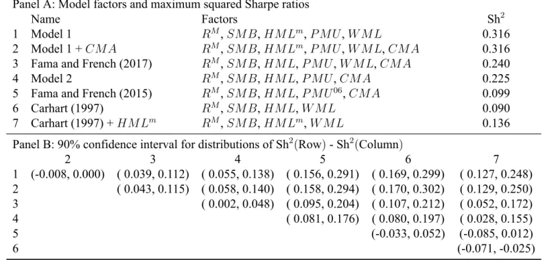
Table 1: Maximum Sharpe ratio and 90% confidence intervals of the distributions of Sh2(Row)−Sh2(Column) from 100,000 bootstrap simulations.
Each bootstrap sample is 654 months drawn randomly with replacement from the 654 months of July 1963-December 2017. In each bootstrap sample, Sh2(f ) is computed for the seven models of Panel A. Panel B shows the matrix of the 5th and 95th percentiles (the 90% confidence interval) of the bootstrap distributions of Sh2(Row)− Sh2(Column), the difference between Sh2(f ) for the row model and Sh2(f ) for the column model. When the 5th and 95th percentiles of the bootstrap distribution of Sh2(Row)− Sh2(Column) are positive, Sh2(Row) is greater than Sh2(Column) in at least 90% of simulation runs, and the 1963-2017 actual Sh2(f ) for
the row model is reliably higher than the 1963-2017 actual Sh2(f ) for the column model. When the 5thand 95thpercentiles of the bootstrap distribution of Sh2(Row)− Sh2(Column) are negative, Sh2(Row) is less than
Sh2(Column) in at least 90% of simulation runs, and the 1963-2017 actual Sh2(f ) for the row model is reliably less than Sh2(f ) for the column model. The factors are constructed as follows. At the end of each June, NYSE, AMEX, and NASDAQ stocks are allocated to two Size groups (small and big) using the NYSE median market-cap breakpoints. Stocks are allocated independently to three BM groups (low to high), using NYSE 30thand 70thpercentile breakpoints. The intersections of the two sorts produce six value-weighted Size-BM portfolios. In the sort for June of year t, B is book equity at the end of the fiscal year ending in year t-1 and M
is market cap at the end of December of year t-1. I use Compustat data to construct book equity, defined as stockholders’ equity (or the par value of preferred plus total common equity or assets minus liabilities) minus the redemption (or liquidation or par value) of preferred stock plus balance sheet deferred taxes. HML is the average of the returns on the two high BM portfolios from the 2x3 sorts minus the average of the returns on the two low BM portfolios. The profitability and investment factors, PMU (profitable minus unprofitable) and CMA (conservative minus aggressive), are formed in the same way as HML, except the second sort variable is cash profitability or investment. Cash profitability, used to create PMU, in the sort for June of year t is measured with accounting data for the fiscal year ending in year t-1 and is revenue minus the cost of goods sold, minus selling, general, and administrative expenses, minus interest expense, plus research and development costs, minus accruals (∆receivables - ∆inventories - ∆pre-paid expenses + ∆deferred revenues + ∆trade payables + ∆accrued expenses) all divided by book equity. Investment, Inv, is the change in total assets from the fiscal year ending in year t-2 to the fiscal year ending in t-1, divided by t-2 total assets. The momentum factor, WML, is defined in the same way as HML, except the factor is updated monthly rather than annually. To form the six Size-Prior portfolios at the end of month t-1, Size is the market cap of a stock at the end of t-1 and Prior is its cumulative return for the 11 months from t-12 to t-2. Monthly value, HM Lm, is defined in the same way as WML except book equity is only updated at the end of June.
Panel A: Model factors and maximum squared Sharpe ratios
Name Factors Sh2
1 Model 1 RM, SM B, HM Lm, P M U , W M L 0.316
2 Model 1 + CM A RM, SM B, HM Lm, P M U , W M L, CM A 0.316 3 Fama and French (2017) RM, SM B, HM L, P M U , W M L, CM A 0.240
4 Model 2 RM, SM B, HM L, P M U , CM A 0.225
5 Fama and French (2015) RM, SM B, HM L, P M U06, CM A 0.099
6 Carhart (1997) RM, SM B, HM L, W M L 0.090
7 Carhart (1997) + HM Lm RM, SM B, HM Lm, W M L 0.136
Panel B: 90% confidence interval for distributions of Sh2(Row) - Sh2(Column)
2 3 4 5 6 7 1 (-0.008, 0.000) ( 0.039, 0.112) ( 0.055, 0.138) ( 0.156, 0.291) ( 0.169, 0.299) ( 0.127, 0.248) 2 ( 0.043, 0.115) ( 0.058, 0.140) ( 0.158, 0.294) ( 0.170, 0.302) ( 0.129, 0.250) 3 ( 0.002, 0.048) ( 0.095, 0.204) ( 0.107, 0.212) ( 0.052, 0.172) 4 ( 0.081, 0.176) ( 0.080, 0.197) ( 0.028, 0.155) 5 (-0.033, 0.052) (-0.085, 0.012) 6 (-0.071, -0.025) 7
Analysis
Table 1 shows the maximum Sh2 for models 1 and 2 as well as five other popular models. Additional models are based on the five-factor model of Fama and French (2015) or the four-factor model of Carhart (1997). Nested models show incremental benefits to adding four-factors. Non-nested models highlight the importance of value and momentum and provide contrast in Sharpe and GRS evidence. The main message of table 1 is that the Sharpe ratio of model 1 is higher than that of model 2 and cannot be improved by adding the investment factor. Model 1 has the lowest mispricing for all portfolios.
Panel A shows the Sh2of model 1 is 0.316 and this is not increased by adding the investment factor, CMA. The Sh2 of model 2 is 0.225 although this can be increased to 0.24 by including the momentum factor. The Sh2of the original Fama and French five-factor model is 0.099. The original Carhart four-factor model has a Sh2of 0.09 although this is increased to 0.136 by updat-ing the value factor monthly. The combination of monthly value and momentum in the modified four-factor model gives a higher Sharpe ratio than the combination of value, operating profitabil-ity and investment in the original five-factor model. This is striking because profitabilprofitabil-ity and investment are credited with reducing the number and maginitude of many common anomalies (Fama and French 2015). Furthermore, profitability and investment slopes provide a unify-ing description of anomalies not constructed from sorts on the factor variables. The returns on problem sorts behave like the returns on small, unprofitable stocks that somehow invest aggres-sively (Fama and French 2016b). The combination of monthly value and momentum has lower mispricing for the returns on all portfolios than profitability and investment.
Panel B shows, generally, those models with a higher Sh2 than another model in panel A have 90% confidence intervals that are strictly positive. For example, the 5th percentile of Sh2(model 1)−Sh2(model 2) is 0.055 and the 95this 0.138. Both percentiles are positive
mean-ing at least 90% of values are positive and the Sh2of model 1 is reliably higher than that of model 2. Any confidence intervals that cross zero imply that neither model is reliably better than the other. The time series of returns that are observed from July 1963 to December 2017 and used to create the Sh2s in panel A may not represent the “true” ranking of the models. For example, the four-factor model that rebalances value monthly may not be truly better than the original five-factor model, despite a higher Sh2 in panel A. The bootstrap procedure produced a significant number of combinations of months where the five-factor model outperformed the four-factor model. Momentum goes through “crashes” or periods of very poor performance (Daniel and Moskowitz 2016; Barroso and Santa-Clara 2015). The bootstrap procedure will produce com-binations of months that include many of the crash months for momentum. The presence of enough momentum crashes, despite the four-factor model with monthly value’s higher Sh2 in panel A, could drive the inconclusive confidence interval with the original five-factor model in panel B. There is no such uncertainty for models 1 and 2 even though model 1 utilizes the same monthly value and momentum relationship as the four-factor model with monthly value. Despite crashes in the momentum factor, model reliably 1 provides the highest Sh2.
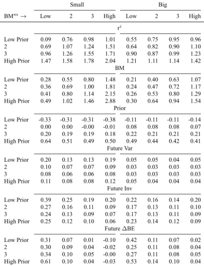
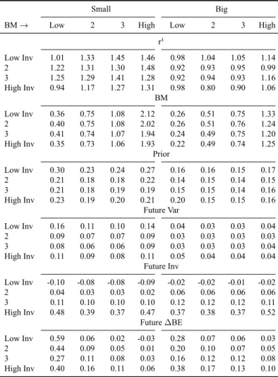
Value and momentum subsume investment and negate any contribution to Sh2(model 1). This is shown by regressing investment on value, annual or monthly, and momentum (not shown). There is no intercept meaning there is no average unexplained return. To explore why this is the case, I sort on value and momentum as well as value and investment and interpret the variation in different characteristics. Table 2 shows average value-weighted characteristics for 32 size-BMm-Prior portfolios and table 3 shows average value-weighted characteristics for 32 size-BM-Inv portfolios. The main message of the tables is that monthly value and momentum’s relationship with small, growth stocks’ future change in BE is the opposite that of annual value and investment. Monthly value and momentum are a better proxy for changes in BE than
Table 2: Value-weighted summary characteristics for sorts on size, monthly value and momentum. At the end of each month, stocks are allocated to two Size groups (Small and Big) using the NYSE median as the ME breakpoint. Small and big stocks are allocated independently to four value buckets (Low BMmto High BMm) and four momentum buckets (Low Prior to High Prior), using NYSE BMmand Prior breakpoints
for the small or big Size group. The intersections of the three sorts produce 32 Size-BMm-Prior portfolios. Each month, characteristics are
value-weighted using the previous month’s ME because value and momentum are updated monthly. Summary characteristics are shown for gross return (ri), monthly value (BMm), annual value (BM), momentum (Prior), cash profitability (CP), future variance (Future Var), future
investment (Future Inv) and future changes in BE (Future ∆BE). Variance is defined as the variance in the prior month’s daily returns.
Small Big
BMm→ Low 2 3 High Low 2 3 High
ri Low Prior 0.09 0.76 0.98 1.01 0.55 0.75 0.95 0.96 2 0.69 1.07 1.24 1.51 0.64 0.82 0.90 1.10 3 0.96 1.26 1.55 1.71 0.90 0.87 0.99 1.23 High Prior 1.47 1.58 1.78 2.04 1.21 1.11 1.14 1.42 BM Low Prior 0.28 0.55 0.80 1.48 0.21 0.40 0.63 1.07 2 0.36 0.69 1.00 1.81 0.24 0.47 0.72 1.17 3 0.41 0.80 1.14 2.15 0.26 0.53 0.80 1.29 High Prior 0.49 1.02 1.46 2.88 0.30 0.64 0.94 1.54 Prior Low Prior -0.33 -0.31 -0.31 -0.38 -0.11 -0.11 -0.11 -0.14 2 0.00 0.00 -0.00 -0.01 0.08 0.08 0.08 0.07 3 0.20 0.19 0.19 0.18 0.22 0.21 0.21 0.21 High Prior 0.64 0.51 0.49 0.50 0.49 0.44 0.42 0.41 Future Var Low Prior 0.20 0.13 0.13 0.19 0.05 0.05 0.04 0.05 2 0.10 0.07 0.07 0.09 0.03 0.03 0.03 0.03 3 0.08 0.06 0.06 0.08 0.03 0.03 0.03 0.03 High Prior 0.11 0.08 0.08 0.12 0.05 0.04 0.04 0.04 Future Inv Low Prior 0.39 0.25 0.19 0.20 0.22 0.16 0.14 0.20 2 0.27 0.16 0.11 0.09 0.17 0.13 0.11 0.10 3 0.24 0.13 0.09 0.07 0.17 0.13 0.11 0.09 High Prior 0.25 0.12 0.10 0.06 0.23 0.14 0.12 0.09 Future ∆BE Low Prior 0.31 0.07 0.01 -0.10 0.42 0.11 0.07 0.02 2 0.30 0.09 0.04 -0.02 0.25 0.11 0.08 0.04 3 0.34 0.10 0.05 -0.00 0.27 0.11 0.08 0.05 High Prior 0.61 0.10 0.04 -0.03 0.53 0.14 0.10 0.04
ment. For monthly value and momentum, small, growth stocks’ future change in BE increases from 0.31 to 0.61 as momentum buckets increase. For annual value and investment, this rela-tionship is reversed as small, growth stocks’ future change in BE decreases from 0.59 to 0.4 as investment buckets increase. The variation in characteristics in table 2 drive many of the results for models 1 and 2 in subsets of portfolios. A model has the potential to describe the returns on a given sort where the characteristic used to construct factors are able to create variation in the characteristic used to construct the subset of portfolios. If increasing one characteristic increases another, this will drive a positive and significant regression slope in time series regressions.
low-Table 3: Value-weighted summary characteristics for sorts on size, annual value and investment. At the end of June each year, stocks are allocated to two Size groups (Small and Big) using the NYSE median as the ME breakpoint. Small and big stocks are allocated independently to four value buckets (Low BM to High BM) and four investment buckets (Low Inv to High Inv), using NYSE BM and Inv breakpoints for the small or big Size group. The intersections of the three sorts produce 32 Size-BM-Inv portfolios. Each month, characteristics are value-weighted using the ME from June (adjusted for returns during the holding period) because value and investment are updated annualy Summary characteristics are shown for gross return (ri), monthly value (BMm), annual value (BM), momentum (Prior), cash profitability (CP), future
variance (Future Var), future investment (Future Inv) and future changes in BE (Future ∆BE). Variance is defined as the variance in the prior month’s daily returns.
Small Big
BM→ Low 2 3 High Low 2 3 High ri Low Inv 1.01 1.33 1.45 1.46 0.98 1.04 1.05 1.14 2 1.22 1.31 1.30 1.48 0.92 0.93 0.95 0.99 3 1.25 1.29 1.41 1.28 0.92 0.94 0.93 1.16 High Inv 0.94 1.17 1.27 1.31 0.98 0.80 0.90 1.06 BM Low Inv 0.36 0.75 1.08 2.12 0.26 0.51 0.75 1.33 2 0.40 0.75 1.08 2.02 0.26 0.51 0.76 1.24 3 0.41 0.74 1.07 1.94 0.24 0.49 0.75 1.20 High Inv 0.35 0.73 1.06 1.93 0.22 0.49 0.74 1.25 Prior Low Inv 0.30 0.23 0.24 0.27 0.16 0.16 0.15 0.17 2 0.21 0.18 0.18 0.22 0.14 0.15 0.14 0.15 3 0.21 0.18 0.19 0.19 0.15 0.15 0.14 0.16 High Inv 0.23 0.19 0.20 0.21 0.20 0.15 0.15 0.16 Future Var Low Inv 0.16 0.11 0.10 0.14 0.04 0.03 0.03 0.04 2 0.09 0.07 0.07 0.09 0.03 0.03 0.03 0.03 3 0.08 0.06 0.06 0.09 0.03 0.03 0.03 0.04 High Inv 0.11 0.09 0.08 0.11 0.05 0.04 0.04 0.04 Future Inv Low Inv -0.10 -0.08 -0.08 -0.09 -0.02 -0.02 -0.01 -0.02 2 0.04 0.03 0.03 0.02 0.06 0.06 0.06 0.06 3 0.11 0.10 0.10 0.10 0.12 0.12 0.12 0.11 High Inv 0.48 0.39 0.37 0.47 0.37 0.38 0.37 0.52 Future ∆BE Low Inv 0.59 0.06 0.02 -0.03 0.28 0.07 0.06 0.03 2 0.44 0.09 0.05 0.01 0.20 0.10 0.07 0.05 3 0.27 0.11 0.08 0.03 0.16 0.12 0.12 0.08 High Inv 0.40 0.16 0.11 0.06 0.38 0.17 0.13 0.10
Prior bucket to 2.04 in the small, high-BMm and high-Prior bucket. Returns across BM and Inv buckets range from 1.01 in the big, low-BM and low-Inv bucket to 1.46 in the small, high-BM and low-Inv bucket. The greater variation in returns for size-BMm-Prior portfolios is expected given the interaction between value and momentum. Their interaction is also visible in the variation in returns at each characteristic’s extreme. For example, in low-BMm the variation in returns across Prior buckets is much larger, 0.09 to 1.47 for small stocks and 0.55 to 0.96 for big stocks, than in high-BMm buckets, 1.01 to 2.04 for small stocks and 1.21 to 1.42 for big stocks. The same is true of the variation in returns across BMm buckets in the extreme Prior
buckets. Lower variation of returns across one characteristic in the extreme buckets of the other mirrors findinings in Asness and Frazzini (2013). Higher variation in returns for size, value and momentum sorts provides potential to price more variation in returns than size, value and investment sorts.
For size-BMm-Prior portfolios, BM increases as Prior buckets increase. For example, in the high-BMm bucket, BM increases from 1.48 to 2.88 for small stocks and from 1.07 to 1.54 for big stocks. Variation in BM within BMmbuckets is undesirable because by sorting on value we should keep value characteristics consistent within value buckets. Consider a stock that is in the high-BMm, high-Prior bucket in July, just after annual BM is recalculated. At this point in the year, BMmand BM are probably at their most similar because ME values differ by six months compared to the maximum of eighteen. If a stock has relatively high returns in the following months, high Prior, its BMmwill decrease as market equity increases while book equity is held constant by a lack of new financial statements. For a stock to remain in the high-BMm, high-Prior bucket, it must have had particularly high BM in order for high returns not to drag the BMm down sufficiently to take the stock out of the high-BMm, high- Prior bucket.
For the size-BMm-Prior portfolios, Prior increases uniformly with Prior buckets and is flat across BMm buckets. The spread in Prior is larger for small stocks than big stocks. In the small, growth bucket, Prior rises from -0.33 to 0.64. In the big, growth bucket, Prior rises from -0.11 to 0.49. For the size-BM-Inv portfolios, there is little variation in Prior across either BM or Inv buckets. Small stocks have higher average recent returns than big stocks with all small stock values close to 0.2 while big stock values are close to 0.15. The lack of variation in momentum characteristics means annual value and investment will struggle to price the returns on momentum sorts.
with the average level and variation in variance characteristics greater for small stocks. Variance decreases marginally, from∼0.2 to ∼0.1, with momentum/investment buckets but only in small stocks. For the most part, sorts on value and momentum/investment do not create variation in the variance characteristic. Monthly value and momentum as well as annual value and investment will struggle to price the returns on subsets of portfolios constructed from sorts on variance. The lack of variation in a characteristic designed to capture volatility is counter-intuitive. If anything, I would expect the variance characteristic to be too noisy, rather than not noisy enough, to capture variation in the variance characteristic. This may reflect problems with my specification of variance. I define variance as the variance of the prior month’s daily returns. I could have used a longer window and perhaps omitted the most recent month as is common for constructing the momentum characteristic.
Fama and French (2006) use the dividend discount model to link the profitability and in-vestment factors to firm value. With clean surplus accounting, the dividend discount model says that market equity equals discounted expected future earnings less the future change in BE,
M Et =
∑∞
s=1E(Yt+s − ∆BEt+s)/R
s where Y is earnings and R is the gross discount rate.
Fama and French use change in assets in place of change in book equity. I examine investment and change in BE characteristics to check if investment is indeed a good proxy for changes in BE.
Future investment decreases across both BMm and Prior buckets for both small and large stocks. In contrast to returns, the effects of each characteristic are similar in the extreme buckets of the other. For example, in the low-Prior bucket, Inv decreases from 0.39 to 0.2 for small stocks and remains flat for big stocks. In the high-Prior bucket, Inv decreases from 0.25 to 0.06 for small stocks and from 0.22 to 0.09 for big stocks. In the low-BMm bucket, Inv decreases from 0.39 to 0.25 for small stocks and remains flat for big stocks. In the high-BMmbucket, Inv
decreases from 0.2 to 0.06 for small stocks and from 0.2 to 0.09 for big stocks. The interaction of monthly value and momentum accounts for the variation in Inv in small and big stocks. In size-BM-Inv sorts, Inv increases uniformly across Inv buckets and remains flat across BM buckets. In size-BMm-Prior sorts, future change in BE in the low-BMmbucket increases from 0.31 to 0.61 as Prior increases. In contrast, future change in BE in the low-BM bucket increases as Inv decreases from 0.59 to 0.4 in size-BM-Inv sorts. For both sorts, future change in BE moves in the opposite direction to the Inv characteristic for small, growth stocks. For size-BMm-Prior sorts, Inv increases while future change in BE decreases while for size-BM-Inv sorts, Inv decreases while future change in BE increases. Investment is not an appropriate proxy for changes in BE. Furthermore, value and momentum capture variation in investment and changes in BE.
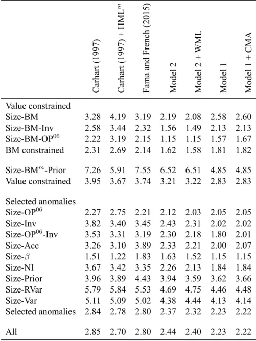
Tables 2 and 3 show model 1 has greater potential to price the returns on many characteristic sorts. Summary characteristics are not bound to regression slopes and a model will struggle where returns do not behave like the characteristics they are constructed from. Table 4 shows the GRS statistic for selected anomalies across the seven models from table 1. A lower GRS statistic indicates less mispricing. As the number of anomaly portfolios increases, the subset of portfolios converges on all portfolios. Consequently, we would expect the GRS statistic evidence for all anomalies to match the Sharpe ratio evidence and this is the case. The main messages of table 4 are that the GRS evidence matches the Sharpe ratio evidence and that momentum and volatility sorts are a problem for all models.
Table 4 includes; value, profitability and investment anomalies (Fama and French 2006; Fama and French 2015); accruals, beta, net issues, momentum and volatility anomalues (Fama and French 2016b); and a sort on size, monthly value and momentum. The anomalies are grouped to illustrate that; constraining annual value hinders the ability of model 1 to price re-turns, constraining monthly value is the least disastrous for model 1, and in sorts on all variables
Table 4: GRS Statistic for selected anomalys sorts, July 1963–December 2017 (654 months).
This table tests how well the models from table 2 explain monthly excess returns on the 25 BM (book-to-market) portfolios, the 25 Size-Acc (accruals) portfolios, the 25 Size-Beta portfolios, the 25 Size-Inv (investment) portfolios, the 35 Size-NI (net share issues) portfolios, the 25 Size-OP (profitability from Fama and French (2006)) portfolios, the 25 Size-Prior 2–12 (momentum) portfolios, the 25 Size-RVar (residual variance) portfolios, the 25 Size-Var (total variance) portfolios, the 32 Size-BM-Inv portfolios, the 32 Size-BM-OP portfolios, the 32 Size-OP-Inv portfolios, and the 32 Size-BMm-Prior (monthly BM). The table shows the GRS statistic testing whether the expected values of all 25, 32,
or 35 intercept estimates are zero.
Carhart (1997) Carhart (1997) + HML m Fama and French (2015) Model 2 Model 2 + WML Model 1 Model 1 + CMA Value constrained Size-BM 3.28 4.19 3.19 2.19 2.08 2.58 2.60 Size-BM-Inv 2.58 3.44 2.32 1.56 1.49 2.13 2.13 Size-BM-OP06 2.22 3.19 2.15 1.15 1.15 1.57 1.67 BM constrained 2.31 2.69 2.14 1.62 1.58 1.81 1.82 Size-BMm-Prior 7.26 5.91 7.55 6.52 6.51 4.85 4.85 Value constrained 3.95 3.67 3.74 3.21 3.22 2.83 2.83 Selected anomalies Size-OP06 2.27 2.75 2.21 2.12 2.03 2.05 2.05 Size-Inv 3.82 3.40 3.45 2.43 2.31 2.02 2.02 Size-OP06-Inv 3.53 3.31 3.19 2.30 2.18 1.80 2.01 Size-Acc 3.26 3.10 3.89 2.33 2.21 2.00 2.07 Size-β 1.51 1.22 1.83 1.63 1.52 1.15 1.15 Size-NI 3.67 3.42 3.35 2.26 2.13 1.84 1.84 Size-Prior 3.96 3.89 4.43 3.94 3.59 3.62 3.66 Size-RVar 5.79 5.84 5.53 4.69 4.75 4.46 4.48 Size-Var 5.11 5.09 5.02 4.38 4.44 4.13 4.14 Selected anomalies 2.84 2.78 2.80 2.37 2.32 2.23 2.22 All 2.85 2.70 2.80 2.44 2.40 2.23 2.22
that are not annual, value model 1 outperforms model 2 (+ WML).
Value compensates for the missing investment factor in model 1. Constraining value limits the variation in value across other characteristics. Model 1, GRS of 1.81, has higher mispricing than model 2, GRS of 1.58, for BM constrained sorts. This impact is particularly evident in size-BM-Inv sorts where the GRS increases from 1.49 for model 2 to 2.13 for model 1. Comparing the GRS for the four-factor models confirms the specification of value, rather than including
momentum, is the problem. The GRS for the original four-factor model with annual value, 2.31, is lower than the GRS for the four-factor model with monthly value, 2.69, for all sorts on BM. The only difference between the two models is the specification of value and this must drive any differences in mispricing.
The size-BMm-Prior sort shows that monthly value and momentum are difficult to price for all models. The GRS for all models is highest for this sort for all models. Model 1 struggles for the size-BMm-Prior sort in an absolute sense, GRS of 4.85. Relative to other models, model 1 performs well. Model 2 has a GRS of 6.52 and the original five-factor model has a GRS of 7.55. Updating the measure of value monthly reduces mispricing more than including the momentum factor. This is shown by the improvement in the GRS, 7.26 to 5.91, from the original four-factor model to the modified four-factor model with monthly value. In contrast, adding momentum to model 2 helps very little. The GRS drops from 6.52 to 6.51.
For all sorts not involving BM, model 1 has the lowest mispricing, GRS of 4.85 for size-BMm-Prior and 2.23 for selected anomalies. This supports Sharpe evidence in table 1 that model 1 minimizes mispricing for all assets. The relatively poor performance of model 1 compared to model 2 for sorts on BM is not enough to cancel out the gains made in all other sorts. The GRS for all sorts is 2.23 for model 1 and 2.44 for model 2. GRS evidence adds colour to the Sharpe ratio bootstrap evidence. For example, table 1 shows Sharpe ratio of the modified four-factor model is not reliably higher than the Sharpe ratio of the original five-factor model but does not indicate why. Table 4 shows Sharpe evidence is not clear beacuse the modified four-factor model has lower mispricing for accruals, beta, and momentum but otherwise underperforms the original five-factor model.
The largest problems for all models are caused by momentum and volatility sorts. Individ-ual regression sorts can help explore why this may be the case by showing which particular
portfolios leave significant alpha. The sign of factor regression slopes will show which end of the factor return spread problem portfolios behave like. For example, a negative profitability slope suggests returns behave like the returns on unprofitable stocks. I focus individual re-gression slopes for models 1 and 2 because they have two of the highest Sharpe ratios and are non-nested.
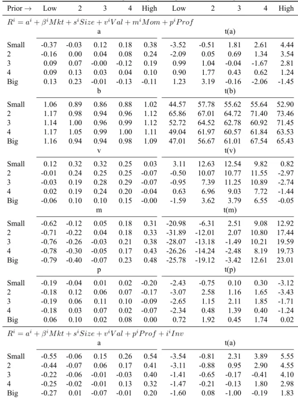
Tables 5 shows 25 time series regressions from size-momentum portfolios for models 1 and 2. Momentum is the tendency for stocks with higher recent returns than their peers to continue to earn higher returns in the short term (Jegadeesh and Titman 1993) and has been found in markets and asset classes throughout the world (Asness, Moskowitz, and Pedersen 2013). The main message of the table is that in the extremes of momentum, value is insignificant and profitability slopes are negative.
Model 1 struggles most with the high-Prior bucket with three significant intercepts out of five. Model 2 has similar problems in the high-Prior bucket but also struggles with the small bucket with four significant intercepts out of five. The small, low-Prior, -0.55, and small, high-Prior, 0.54, intercepts for model 2 are reduced to -0.37 and 0.38 for model 1. Improvements in mispricing for model 1 are due to the negative momentum slopes for low-Prior and positive momentum slopes for high-Prior.
Beta slopes exhibit a smile across momentum buckets. The small bucket has a drop from 1.06 in the low-Prior bucket to 0.86 in the middle Prior bucket before returning to 1.02 in the high-Prior bucket. Similarly, the big bucket has a drop from 1.16 to 0.94 before rising again to 1.09. The extremes of momentum behave like the returns on high-beta stocks. Value slopes exhibit a frown with coefficients remaining∼0.3 in the middle momentum buckets but becoming insignificant in the extreme momentum buckets. The extremes of momentum do not covary with the returns on the value factor. Value does most of the heavy lifting along with profitability and
Table 5: Regressions for the 25 Size-Prior portfolios, July 1963–December 2017 (654 months).
The LHS variables in each set of 25 regressions are the monthly excess returns on the 25 Size-Prior portfolios. The RHS variables are the excess market return, RM, the Size factor, SM B, value factor, HM L(m), the profitability factor, P M U , the momentum factor, W M L, and the
investment factor, CM A. The table shows model 1 intercepts and regression slopes and model 2 intercepts.
Prior→ Low 2 3 4 High Low 2 3 4 High
Ri= ai+ βiM kt + siSize + viV al + miM om + piP rof a t(a) Small -0.37 -0.03 0.12 0.18 0.38 -3.52 -0.51 1.81 2.61 4.44 2 -0.16 0.00 0.04 0.08 0.24 -2.09 0.05 0.69 1.34 3.54 3 0.09 0.07 -0.00 -0.12 0.19 0.99 1.04 -0.04 -1.67 2.81 4 0.09 0.13 0.03 0.04 0.10 0.90 1.77 0.43 0.62 1.24 Big 0.13 0.23 -0.01 -0.13 -0.11 1.23 3.19 -0.16 -2.06 -1.45 b t(b) Small 1.06 0.89 0.86 0.88 1.02 44.57 57.78 55.62 55.64 52.90 2 1.17 0.98 0.94 0.96 1.12 65.86 67.01 64.72 71.40 73.46 3 1.14 1.00 0.96 0.99 1.12 52.72 64.52 62.78 60.92 71.45 4 1.17 1.05 0.99 1.00 1.11 49.04 61.97 60.57 61.84 63.53 Big 1.16 0.94 0.94 0.98 1.09 47.01 56.67 61.01 67.54 65.43 v t(v) Small 0.12 0.32 0.32 0.25 0.03 3.11 12.63 12.54 9.82 0.82 2 -0.01 0.24 0.25 0.25 -0.07 -0.50 10.07 10.77 11.55 -2.97 3 -0.03 0.19 0.28 0.29 -0.07 -0.95 7.39 11.25 10.89 -2.74 4 0.02 0.19 0.24 0.20 -0.04 0.63 6.96 9.03 7.72 -1.44 Big -0.06 0.10 0.10 0.15 -0.00 -1.59 3.62 3.79 6.55 -0.05 m t(m) Small -0.62 -0.12 0.05 0.18 0.31 -20.98 -6.31 2.51 9.08 12.92 2 -0.71 -0.22 0.04 0.18 0.33 -31.89 -12.01 2.07 10.80 17.44 3 -0.76 -0.26 -0.03 0.21 0.38 -28.07 -13.18 -1.49 10.21 19.59 4 -0.78 -0.30 -0.05 0.17 0.43 -26.26 -14.24 -2.48 8.19 19.73 Big -0.79 -0.40 -0.07 0.23 0.48 -25.78 -19.12 -3.42 12.61 23.01 p t(p) Small -0.19 -0.04 0.01 0.02 -0.20 -2.43 -0.75 0.10 0.30 -3.12 2 -0.18 0.12 0.06 0.07 -0.17 -3.07 2.58 1.16 1.65 -3.43 3 -0.19 0.06 0.11 0.10 -0.09 -2.65 1.15 2.11 1.85 -1.71 4 -0.18 0.03 0.07 0.02 -0.07 -2.34 0.48 1.39 0.40 -1.24 Big 0.06 0.10 0.02 0.08 0.00 0.72 1.92 0.45 1.74 0.02 Ri= ai+ βiM kt + siSize + viV al + piP rof + iiInv
a t(a) Small -0.55 -0.06 0.15 0.26 0.54 -3.54 -0.81 2.31 3.89 5.55 2 -0.44 -0.07 0.06 0.17 0.41 -3.11 -0.88 0.95 2.90 4.55 3 -0.22 -0.06 -0.01 -0.03 0.40 -1.41 -0.65 -0.17 -0.41 4.10 4 -0.25 -0.02 -0.01 0.13 0.32 -1.47 -0.21 -0.13 1.80 2.98 Big -0.27 0.01 -0.07 -0.01 0.20 -1.60 0.08 -1.00 -0.19 1.83
there is mispricing in the buckets where value disappears. Momentum slopes increase uniformly
from ∼-0.7 to ∼0.4 as momentum buckets increase, although the spread in slopes is slightly
larger for big stocks than small stocks. Profitability slopes also exhibit a frown but, in contrast to value, are negative and significant in the extremes of momentum but insignificant in the inner
momentum buckets.
Beta and variance are linked as a stock’s variance drives its covariance with the market. The returns on the extremes of momentum, and subsequent mispricing, may be due to low and high-momentum identifying stocks with high volatility. Furthermore, profitability slopes also point to high volatility stocks because profitability helps to describe the returns on “defensive equity” strategies (Novy-Marx 2014). Such strategies focus on low-beta, low-volatility stocks. Momentum’s interaction with volatility characteristics, rather than momentum itself, could drive returns in the extremes of momentum. Value’s weakness in the extremes of momentum may stem from returns behaving like the returns on high-beta and/or high-volatility stocks, rather than low or high-momentum stocks. Next, I investigate mispricing and factor slopes for sorts on beta.
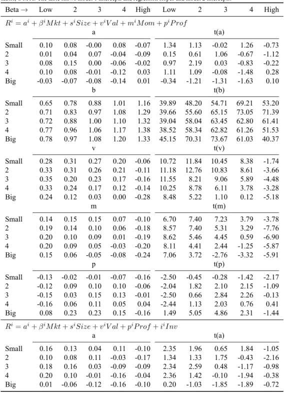
Table 6 shows 25 time series regressions from size-beta portfolios for models 1 and 2. The main messages of the table are that sorts on beta are not a problem for model 1 and value disap-pears in the small, high-beta bucket. The beta characteristics, and volatility characteristics tied to beta, do not drive mispricing in momentum sorts. Positive momentum slopes for model 1 cap-ture the mispricing for model 2 in the low-beta bucket. Where Fama and French (2016b) find that low-beta stocks behave like profitable, conservatively investing stocks, I find that low-beta stocks behave like unprofitable, value stocks with strong recent returns.
Beta slopes increase with size and beta buckets. Big stocks behave more like the return on the market than small stocks. The spread in beta slopes is similar for small and big stocks,∼0.7 to ∼1.3. Value slopes are flat across beta buckets except for a drop in the high-beta bucket. High-beta stocks behave like the returns on growth stocks. Like the small, high-momentum portfolio, value disappears in the small, high-beta portfolio although, unlike momentum, this does not result in mispricing. There is a size effect in value slopes for the high-beta bucket with slopes decreasing from -0.06 for small stocks to -0.28 for big stocks. Momentum slopes decrease
Table 6: Regressions for the 25 Size-Beta portfolios, July 1963–December 2017 (654 months).
The LHS variables in each set of 25 regressions are the monthly excess returns on the 25 Size-Beta portfolios. The RHS variables are the excess market return, RM, the Size factor, SM B, value factor, HM L(m), the profitability factor, P M U , the momentum factor, W M L, and the
investment factor, CM A. The table shows model 1 intercepts and regression slopes and model 2 intercepts.
Beta→ Low 2 3 4 High Low 2 3 4 High
Ri = ai+ βiM kt + siSize + viV al + miM om + piP rof a t(a) Small 0.10 0.08 -0.00 0.08 -0.07 1.34 1.13 -0.02 1.26 -0.73 2 0.01 0.04 0.07 -0.04 -0.09 0.15 0.61 1.06 -0.67 -1.12 3 0.08 0.15 0.00 -0.06 -0.02 0.97 2.19 0.03 -0.83 -0.22 4 0.10 0.08 -0.01 -0.12 0.03 1.11 1.09 -0.08 -1.48 0.28 Big -0.03 -0.07 -0.08 -0.14 0.01 -0.34 -1.21 -1.31 -1.63 0.10 b t(b) Small 0.65 0.78 0.88 1.01 1.16 39.89 48.20 54.71 69.21 53.20 2 0.71 0.83 0.97 1.08 1.29 39.66 55.60 65.15 73.05 71.39 3 0.72 0.88 1.00 1.10 1.32 39.04 58.04 63.45 62.80 61.41 4 0.77 0.96 1.06 1.17 1.38 38.52 58.34 62.82 61.26 51.53 Big 0.78 0.97 1.08 1.20 1.33 45.15 70.31 73.67 61.03 40.37 v t(v) Small 0.28 0.31 0.27 0.20 -0.06 10.72 11.84 10.45 8.38 -1.74 2 0.33 0.31 0.26 0.21 -0.11 11.18 12.76 10.83 8.61 -3.66 3 0.35 0.20 0.23 0.17 -0.16 11.55 8.21 9.06 5.89 -4.48 4 0.33 0.24 0.17 0.12 -0.14 10.25 8.78 6.11 3.78 -3.28 Big 0.24 0.12 0.03 0.00 -0.28 8.48 5.22 1.10 0.12 -5.18 m t(m) Small 0.14 0.15 0.15 0.07 -0.10 6.70 7.40 7.23 3.79 -3.78 2 0.19 0.14 0.10 0.06 -0.18 8.57 7.40 5.31 3.29 -7.76 3 0.20 0.10 0.09 0.01 -0.19 8.62 5.46 4.45 0.59 -6.90 4 0.20 0.09 0.05 -0.03 -0.20 8.11 4.41 2.44 -1.25 -5.87 Big 0.15 0.06 -0.05 -0.08 -0.24 7.06 3.72 -2.76 -3.32 -5.91 p t(p) Small -0.13 -0.02 -0.01 -0.07 -0.16 -2.50 -0.45 -0.28 -1.42 -2.17 2 -0.12 0.09 0.10 0.10 -0.06 -2.04 1.82 2.10 2.15 -1.09 3 -0.15 0.03 0.15 0.13 -0.01 -2.50 0.66 2.84 2.26 -0.13 4 -0.16 0.06 0.11 0.05 0.04 -2.44 1.13 2.03 0.76 0.41 Big 0.08 0.23 0.23 0.15 -0.16 1.49 5.05 4.86 2.31 -1.44 Ri = ai+ βiM kt + siSize + viV al + piP rof + iiInv
a t(a) Small 0.16 0.13 0.04 0.11 -0.10 2.35 1.96 0.65 1.84 -1.05 2 0.10 0.08 0.11 -0.03 -0.17 1.34 1.33 1.75 -0.43 -2.16 3 0.18 0.16 0.03 -0.09 -0.09 2.34 2.59 0.48 -1.17 -0.98 4 0.20 0.10 -0.01 -0.16 -0.04 2.36 1.42 -0.10 -1.94 -0.38 Big 0.01 -0.06 -0.12 -0.16 -0.10 0.20 -1.03 -1.85 -1.89 -0.72
as beta buckets increase. Low-beta stocks behave like stocks with strong recent returns, while high-beta stocks behave like stocks with poor recent returns. This contradicts table 5 that shows that low and high-momentum stocks behave like the returns on high-beta stocks. Like value, there is a size effect in momentum slopes for the high-beta bucket with slopes decreasing from
-0.1 for small stocks to -0.24 for big stocks. Profitability slopes are largely insignificant except for the low-beta bucket and the small, high-beta portfolio. Profitability slopes are negative for the low-beta bucket and this makes sense given profitability’s relationship with defensive equity. Beta and profitability slopes in table 5 point to a shared story for momentum and volatility. Table 6 shows that beta itself, and volatility tied to beta, is not the problem. In fact, table 4 shows that sorts on beta cause the least problems of all sorts tested, GRS of 1.15 for model 1. Beta’s lack of mischief is important because of the historical stubbornness of the anomaly (Jensen, Black, and Scholes 1972). Model 1 drives out alphas in low-beta portfolios. Next, I investigate mispricing and factor slopes for sorts on variance.
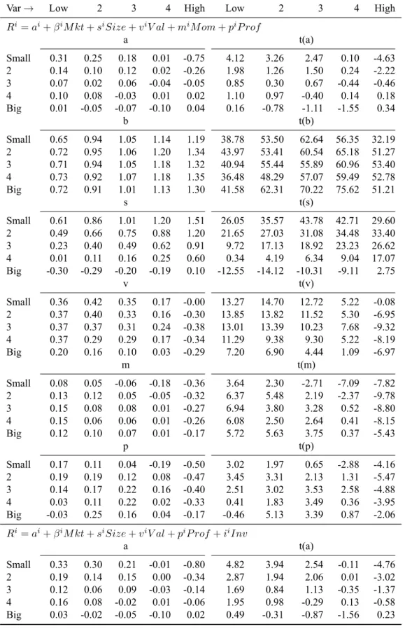
Table 7 shows 25 time series regressions from size-variance sorts for models 1 and 2. The main message of the table is that stocks that share the “lethal combination” of negative prof-itability and investment slopes behave like unprofitable stocks with poor recent returns. Like momentum sorts, the portfolios with the most mispricing coincide with value’s disappearance. Those sorts that create problems for model 1 have returns that do not covary with the returns on the value factor.
In contrast to momentum and beta sorts, there is no significant improvement in the magnitude of the alphas. The small, high-Var portfolio has an alpha of -0.75 for model 1 and -0.8 for model 2. Beta increases as volatility buckets increase and remains flat across size buckets. The relationship with beta makes sense given individual portfolio variance drives covariance with the market. Despite controlling for size slopes increase with volatility buckets. In the smallest two size buckets, the variation in size slopes is extreme. The smallest size bucket slopes rise from 0.63 to 1.5 and the second size bucket slopes rise from 0.51 to 1.18. The importance of size slopes corresponds with characteristic evidence in table 2 that shows greater variation in the variance characteristic for small stocks. Positive value slopes show that low-Var stocks behave like the
Table 7: Regressions for the 25 Size-Var portfolios, July 1963–December 2017 (654 months).
The LHS variables in each set of 25 regressions are the monthly excess returns on the 25 Size-Var portfolios. The RHS variables are the excess market return, RM, the Size factor, SM B, value factor, HM L(m), the profitability factor, P M U , the momentum factor, W M L, and the
investment factor, CM A. The table shows model 1 intercepts and regression slopes and model 2 intercepts.
Var→ Low 2 3 4 High Low 2 3 4 High
Ri= ai+ βiM kt + siSize + viV al + miM om + piP rof a t(a) Small 0.31 0.25 0.18 0.01 -0.75 4.12 3.26 2.47 0.10 -4.63 2 0.14 0.10 0.12 0.02 -0.26 1.98 1.26 1.50 0.24 -2.22 3 0.07 0.02 0.06 -0.04 -0.05 0.85 0.30 0.67 -0.44 -0.46 4 0.10 0.08 -0.03 0.01 0.02 1.10 0.97 -0.40 0.14 0.18 Big 0.01 -0.05 -0.07 -0.10 0.04 0.16 -0.78 -1.11 -1.55 0.34 b t(b) Small 0.65 0.94 1.05 1.14 1.19 38.78 53.50 62.64 56.35 32.19 2 0.72 0.95 1.06 1.20 1.34 43.97 53.41 60.54 65.18 51.27 3 0.71 0.94 1.05 1.18 1.32 40.94 55.44 55.89 60.96 53.40 4 0.73 0.92 1.07 1.18 1.35 36.48 48.29 57.07 59.49 52.78 Big 0.72 0.91 1.01 1.13 1.30 41.58 62.31 70.22 75.62 51.21 s t(s) Small 0.61 0.86 1.01 1.20 1.51 26.05 35.57 43.78 42.71 29.60 2 0.49 0.66 0.75 0.88 1.20 21.65 27.03 31.08 34.48 33.40 3 0.23 0.40 0.49 0.62 0.91 9.72 17.13 18.92 23.23 26.62 4 0.01 0.11 0.16 0.25 0.60 0.34 4.19 6.34 9.04 17.07 Big -0.30 -0.29 -0.20 -0.19 0.10 -12.55 -14.12 -10.31 -9.11 2.75 v t(v) Small 0.36 0.42 0.35 0.17 -0.00 13.27 14.70 12.72 5.22 -0.08 2 0.37 0.40 0.33 0.16 -0.30 13.85 13.82 11.52 5.30 -6.95 3 0.37 0.37 0.31 0.24 -0.38 13.01 13.39 10.23 7.68 -9.32 4 0.37 0.29 0.29 0.17 -0.34 11.29 9.38 9.30 5.22 -8.19 Big 0.20 0.16 0.10 0.03 -0.29 7.20 6.90 4.44 1.09 -6.97 m t(m) Small 0.08 0.05 -0.06 -0.18 -0.36 3.64 2.30 -2.71 -7.09 -7.82 2 0.13 0.12 0.05 -0.05 -0.32 6.37 5.48 2.19 -2.37 -9.78 3 0.15 0.08 0.08 0.01 -0.27 6.94 3.80 3.28 0.52 -8.80 4 0.15 0.06 0.06 0.01 -0.26 6.08 2.50 2.64 0.41 -8.15 Big 0.12 0.10 0.07 0.01 -0.17 5.72 5.63 3.75 0.37 -5.43 p t(p) Small 0.17 0.11 0.04 -0.19 -0.50 3.02 1.97 0.65 -2.88 -4.16 2 0.19 0.19 0.12 0.08 -0.47 3.45 3.31 2.13 1.31 -5.47 3 0.14 0.17 0.22 0.16 -0.40 2.51 3.02 3.53 2.58 -4.88 4 0.03 0.11 0.22 0.02 -0.33 0.41 1.83 3.49 0.36 -3.95 Big -0.03 0.25 0.16 0.04 -0.17 -0.46 5.13 3.39 0.87 -2.06 Ri= ai+ βiM kt + siSize + viV al + piP rof + iiInv
a t(a) Small 0.33 0.30 0.21 -0.01 -0.80 4.82 3.94 2.54 -0.11 -4.76 2 0.19 0.14 0.15 0.00 -0.34 2.87 1.94 2.06 0.01 -3.02 3 0.12 0.06 0.09 -0.03 -0.14 1.69 0.84 1.13 -0.35 -1.37 4 0.16 0.08 -0.02 0.01 -0.06 1.95 0.98 -0.29 0.13 -0.58 Big 0.03 -0.02 -0.05 -0.10 0.02 0.49 -0.31 -0.87 -1.56 0.23
returns on value stocks. Negative value slopes show that high-Var stocks behave like the returns on growth stocks. The value slope is insignificant in the small, high-Var bucket. Momentum slopes are negative for the high-Var bucket,∼-0.3, but otherwise remain low, ∼0.1. The returns on high-Var stocks behave like the returns on stocks with poor recent returns. Profitability slopes are negative for the high-Var bucket and increase with size buckets from -0.5 for small stocks to -0.17 for big stocks. The returns on low-Var stocks behave like unprofitable stocks. The remaining profitability slopes are positive and∼0.15. Sorts on variance are a major problem, as shown by the -0.75% alpha per month in the small, high-Var portfolio. Variance is related to beta but the component of variance associated with returns on the market does not cause problems for model 1, as shown by the insignificant alphas in table 6.
To take advantage of the alpha in the small, high-Var bucket of table 7, an investor has to sell stocks whose returns behave like those of small, unprofitable firms with poor recent returns. Nagel (2005) writes “for mis-pricing to persist in the in the presence of [smart money], limits to arbtrage must exist”. small, unprofitable firms with poor recent returns are likely more illiquid than than big, profitable stocks with strong recent returns. Furthermore, small stocks are likely to be held by fewer institutional investors or “market makers” willing to provide the other side of a trade for arbitrageurs. Nagel (2012) uses the short-term reversal strategy to proxy for the returns to market makers who represent the largest group of buyers for problem stocks. Nagel finds liquidity measured in this way is related to the aggregate level of volatility, proxied by the VIX. There may be a large alpha for the small, high-Var portfolio because noone is willing to buy from arbitrageurs trying to sell small, high-Var stocks.
Corresponding with my findings that value disappears in the small, high-Var portfolio, As-ness, Liew, et al. (2018) find that volatility increases during periods of “deep value”. Deep value means the spread between the value characteristic of cheap and expensive stocks is large.
During a deep value event, the returns on the spread between cheap and expensive stocks is higher, volatility is higher and the earnings of cheap stocks are particularly low compared to normal times. Asness et al. also find illiquidity indicators such as short interest and analysts re-visions of forecasts are increased during periods of deep value. Value’s disappearance seems to coincide with an increase in illiquidity that makes selling small, high-Var stocks difficult. With-out arbitrageurs selling small, high-Var stocks, there is no price correction and inflated prices remain.
Nevertheless, liquidity explanations are not easy to tackle from a cross-section perspective and often focus on market microstructure such as market makers and analysts’ forecasts revi-sions. Furthermore, Ang et al. (2006) test many possible liquidity explanations3for the volatil-ity anomaly from a cross-section perspective and find none help greatly to price the returns on highly volatile stocks. They also find that the aggregate level of volatility, proxied for by the VIX, does not drive out alphas in sorts on volatility. Liquidity, through aggregate volatility or deep value, is not the cause of alpha in small, high-volatility stocks.
I use value’s disappearance as a starting point for a cross-section explanation for the problems with small, high-Var portfolios. Value is a noisy proxy because BE and ME are imprecise ways to describe firms. Furthermore, BE and ME are explicitly part of other factors, for example profitability and size. Value can be “cleaned up” with momentum but prior research finds there is more to value than simply BE and ME4. Gerakos and Linnainmaa (2017) note that much of
the value factor relates to changes in firm size and split the factor into size-driven value and non-size-driven, “orthogonal” value. They find that not all high-BM firms make the value premium and some low-BM firms do make the value premium. This observation does not render the value factor useless, but it does help to illustrate that the value premium is not the same as the
3Bid-ask spreads, trading volume, and turnover, among others.
“empirical regularity that average returns increase in BM ratios”. Further, size-driven value is more related to variance than orthogonal value. I find the alpha in the small, high-Var bucket disappears for both models when the size factor is omitted (not shown). Omitting the size factor results in negative value slopes suggesting that, without size clouding the issue, small, high-Var stocks behave like unprofitable, growth stocks with poor recent returns just as table 6 shows for small, high-beta stocks. Small, high-Var firms have poor returns but the size factor pushes up the predicted return from the model. Furthermore, the size factor subsumes the value factor negating the value slopes that could pull the predicted return from the model down and reduce mispricing. In keeping with the top-down approach, this does not mean the size factor should be removed from the model. Rather, the model provides a description of the problem. The returns on small, high-Var stocks behave like the returns on small, unprofitable stocks with poor recent performance. Mispricing stems from firm size, through the relationship between size and volatility, and not illiquidity, as has been the focus of prior research. This is evident directly through the size slope inflating the predicted return from model 1 as well as indirectly through value’s disappearance in problem buckets.
Conclusions
Barillas and Shanken’s observation that maximizing the Sharpe ratio of an asset-pricing model minimizes mispricing for all portfolios enables a top-down approach to choosing factors. Com-paring the Sharpe ratio of models before testing mispricing for subsets of portfolios promotes intuition over statistics and helps fight against data-mining. The model with the least mispric-ing for all portfolios provides a description of problem portfolios, rather than problem portfolios driving the choice of factors.
A five-factor model of market, size, value, momentum and profitability factors has a
imum squared Sharpe ratio of 0.316. This is not improved by including the investment fac-tor. Investment is subsumed by value and momentum because it is an inferior proxy for future changes in book equity. GRS evidence for subsets of portfolios confirms Sharpe ratio evidence and highlights the problems with momentum and volatility sorts. My proposed model shows the previous “lethal combination” of unprofitable firms that somehow invest aggressively is described by unprofitable firms with poor recent returns. Value’s disappearance for problem sorts coincides with volatility problems. Size factor slopes, compounded by the size-driven component of value’s relationship with volatility, drive mispricing for volatile stocks and point to problems with firm size beyond illiquidity. My findings promote further research into the relationship between value and volatility.
References
Ang, Andrew et al. (2006). “The cross-section of volatility and expected returns”. In: The
Jour-nal of Finance 61.1, pp. 259–299.
Asness, Clifford S, John M Liew, et al. (2018). “Deep value”. In: :https://ssrn.com/ abstract=3122327.
Asness, Clifford S, Tobias J Moskowitz, and Lasse Heje Pedersen (2013). “Value and momentum everywhere”. In: The Journal of Finance 68.3, pp. 929–985.
Asness, Clifford and Andrea Frazzini (2013). “The devil in HML’s details”. In: The Journal of
Portfolio Management 39.4, pp. 49–68.
Ball, Ray et al. (2016). “Accruals, cash flows, and operating profitability in the cross section of stock returns”. In: Journal of Financial Economics 121.1, pp. 28–45.
Barillas, Francisco and Jay Shanken (2016). “Which alpha?” In: The Review of Financial Studies 30.4, pp. 1316–1338.
Barroso, Pedro and Pedro Santa-Clara (2015). “Momentum has its moments”. In: Journal of
Financial Economics 116.1, pp. 111–120.
Carhart, Mark M (1997). “On persistence in mutual fund performance”. In: The Journal of
fi-nance 52.1, pp. 57–82.
Cohen, Randolph B, Christopher Polk, and Tuomo Vuolteenaho (2003). “The value spread”. In:
The Journal of Finance 58.2, pp. 609–641.
Daniel, Kent and Tobias J Moskowitz (2016). “Momentum crashes”. In: Journal of Financial
Economics 122.2, pp. 221–247.
Daniel, Kent and Sheridan Titman (2006). “Market reactions to tangible and intangible infor-mation”. In: The Journal of Finance 61.4, pp. 1605–1643.
Fama, Eugene F and Kenneth R French (1992). “The cross-section of expected stock returns”. In: the Journal of Finance 47.2, pp. 427–465.
— (2006). “Profitability, investment and average returns”. In: Journal of Financial Economics 82.3, pp. 491–518.
Fama, Eugene F and Kenneth R French (2008). “Average returns, B/M, and share issues”. In:
The Journal of Finance 63.6, pp. 2971–2995.
— (2015). “A five-factor asset pricing model”. In: Journal of Financial Economics 116, pp. 1– 22.
— (2016a). “Choosing factors”. In: :https://ssrn.com/abstract=2834871.
— (2016b). “Dissecting anomalies with a five-factor model”. In: The Review of Financial
Stud-ies 29.1, pp. 69–103.
Gerakos, Joseph and Juhani T Linnainmaa (2017). “Decomposing value”. In: The Review of
Financial Studies 31.5, pp. 1825–1854.
Gibbons, Michael R, Stephen A Ross, and Jay Shanken (1989). “A test of the efficiency of a given portfolio”. In: Econometrica: Journal of the Econometric Society, pp. 1121–1152. Graham, Benjamin and David L Dodd (1934). Security analysis: Principles and technique.
McGraw-Hill.
Harvey, Campbell R, Yan Liu, and Heqing Zhu (2016). “… and the cross-section of expected returns”. In: The Review of Financial Studies 29.1, pp. 5–68.
Jegadeesh, Narasimhan and Sheridan Titman (1993). “Returns to buying winners and selling losers: Implications for stock market efficiency”. In: The Journal of finance 48.1, pp. 65– 91.
Jensen, Michael C, Fischer Black, and Myron S Scholes (1972). “The capital asset pricing model: Some empirical tests”. In:
Kok, U-Wen, Jason Ribando, and Richard Sloan (2017). “Facts about Formulaic Value Invest-ing”. In: Financial Analysts Journal 73.2, pp. 81–99.
Linnainmaa, Juhani T and Michael R Roberts (2016). The history of the cross section of stock
returns. Tech. rep. National Bureau of Economic Research.
Moreira, Alan and Tyler Muir (2017). “Volatility-Managed Portfolios”. In: The Journal of
Fi-nance 72.4, pp. 1611–1644.
Nagel, Stefan (2005). “Short sales, institutional investors and the cross-section of stock returns”. In: Journal of Financial Economics 78.2, pp. 277–309.
— (2012). “Evaporating liquidity”. In: The Review of Financial Studies 25.7, pp. 2005–2039. Novy-Marx, Robert (2014). Understanding defensive equity. Tech. rep. National Bureau of
Eco-nomic Research.
Variables
Characteristics are given by the following formulas
• Monthly Return: RET = (1 + RET )(1 + DLRET )− 1 • Market Equity: M E = SHROU T · abs(P RC)/1000
• Book Equity: BE = seq + txditc− ps where ps equals (in order of preference); pstkrv,
pstkl or pstk. If all measures of preferred stock are missing, BE = ceq + upstk. If we
still do not have a value for BE, BE = at− lt
• Book-to-Market: BE/M E where M E is either from December, Fama and French (1992) or month t− 1, Asness and Frazzini (2013).
• Profitability: OP = (revt−cogs−xsga−xint)/BE. Fama and French (2016a) add back research and development costs to OP , OPr = (revt− cogs − xsga − xint + xrd)/BE
and CP = (revt− cogs − xsga − xint + xrd + acc)/BE where (Ball et al. 2016)
acc =−∆rect − ∆invt − ∆xpp + ∆drc + ∆ap + ∆xacc
• Investment: Inv = (att− att−1)/att−1
where the full description of the codes are (capital letters denote CRSP while lower-case letters denote COMPUSTAT)
• EXCHCD: Exchange Code (1-NSYE, 2-AMEX, 3-NASDAQ) • PRC: Share Price
• SHROUT: Number of Shares Outstanding • RET: Monthly Return
• DLRET: De-listing Return • at: Total Assets
• xpp: Prepaid Expenses • invt: Total Inventory • rect: Total Receivables • lt: Total Liabilities
• ap: Accounts Payable - Trade • drc: Deferred Revenue • xacc: Accrued Expenses • seq: Stockholder’s Equity
• ceq: Book Value of Common Equity • txditc: Deferred Taxes
• pstkrv: Preferred Stock (PS), Redemption Value • pstkl: PS, Liquidation Value
• pstk: PS, Book Value • upstk: PS, Par Value
• revt: Total Revenue (This is the same as sale for US firms) • cogs: Cost of Goods Sold
• xsga: Selling, General and Administrative • xrd: Research and Development Costs • xint: Total Interest Expenses
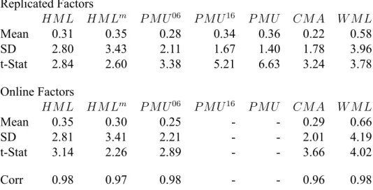
Table 8: Monthly averages, standard deviations, t-statistics and correlations with factors available from previous research for replicated factor returns, July 1963 - December 2017 (654 months). At the end of each June, NYSE, AMEX, and NASDAQ stocks are allocated to two Size groups (small and big) using the NYSE median market-cap breakpoints. Stocks are allocated independently to three B/M groups (low to high), using NYSE 30thand 70thpercentile breakpoints. The intersections of the two sorts produce six value-weight Size-B/M portfolios. In
the sort for June of year t, B is book equity at the end of the fiscal year ending in year t-1 and M is market cap at the end of December of year t-1. I use Compustat data to compute book equity, defined as (1) stockholders’ equity (or the par value of preferred plus total common equity or assets minus liabilities, in that order) minus (2) the redemption, liquidation, or par value of preferred (in that order) plus (3) balance sheet deferred taxes. HML is the average of the returns on the two high B/M portfolios from the 2x3 sorts minus the average of the returns on the two low B/M portfolios. The profitability and investment factors, PMU (profitable minus unprofitable) and CMA (conservative minus aggressive), are formed in the same way as HML, except the second sort variable is operating profitability or investment. Operating profitability, used to create P M U06, in the sort for June of year t is measured with accounting data for the fiscal year ending in year t-1 and is revenue minus the
cost of goods sold, minus selling, general, and administrative expenses, minus interest expense, all divided by book equity. Adjusted operating profitability, P M U16, is created similarly except research and development costs are added back in before dividing by book equity. Cash
profitbality, P M U , is created by subtracting accruals before dividing by book equity. Investment, Inv, is the change in total assets from the fiscal year ending in year t-2 to the fiscal year ending in t-1, divided by t-2 total assets. The momentum factor, WML, is defined in the same way as HML, except the factor is updated monthly rather than annually. To form the six Size- Prior 2-12 portfolios at the end of month t-1, Size is the market cap of a stock at the end of t-1 and Prior 2-12 is its cumulative return for the 11 months from t-12 to t-2. Monthly value, HM Lm, is defined in the same way as WML except book equity is only updated at the end of June.
Replicated Factors HM L HM Lm P M U06 P M U16 P M U CM A W M L Mean 0.31 0.35 0.28 0.34 0.36 0.22 0.58 SD 2.80 3.43 2.11 1.67 1.40 1.78 3.96 t-Stat 2.84 2.60 3.38 5.21 6.63 3.24 3.78 Online Factors HM L HM Lm P M U06 P M U16 P M U CM A W M L Mean 0.35 0.30 0.25 - - 0.29 0.66 SD 2.81 3.41 2.21 - - 2.01 4.19 t-Stat 3.14 2.26 2.89 - - 3.66 4.02 Corr 0.98 0.97 0.98 - - 0.96 0.98
Replication
Table 8 shows summary statistics for constructed and online factors. The main message of the table is that my results can be believed. Values should be compared to Kenneth French’s website for all factors except HM Lm, which should be compared to data available from AQR Captial Management. All factors are significant and highly correlated with their “true” online counter-parts.