FAST AND ADAPTIVE SURFACE RECONSTRUCTION FROM MOBILE LASER
SCANNING DATA OF URBAN AREAS
M. Gordon∗, M. Hebel, M. Arens
Fraunhofer Institute of Optronics, System Technologies and Image Exploitation IOSB Ettlingen, Germany
[email protected], [email protected], [email protected] http://www.iosb.fraunhofer.de
KEY WORDS:LIDAR, Mapping, Mobile laser scanning, Urban, Surface reconstruction
ABSTRACT:
The availability of 3D environment models enables many applications such as visualization, planning or simulation. With the use of current mobile laser scanners it is possible to map large areas in relatively short time. One of the emerging problems is to handle the resulting huge amount of data. We present a fast and adaptive approach to represent connected 3D points by surface patches while keeping fine structures untouched. Our approach results in a reasonable reduction of the data and, on the other hand, it preserves details of the captured scene. At all times during data acquisition and processing, the 3D points are organized in an octree with adaptive cell size for fast handling of the data. Cells of the octree are filled with points and split into subcells, if the points do not lie on one plane or are not evenly distributed on the plane. In order to generate a polygon model, each octree cell and its corresponding plane are intersected. As a main result, our approach allows the online generation of an expandable 3D model of controllable granularity. Experiments have been carried out using a sensor vehicle with two laser scanners at an urban test site. The results of the experiments show that the demanded compromise between data reduction and preservation of details can be reached.
1. INTRODUCTION
3D environment models are required for multiple purposes in the area of planning and simulation. One of the established ways to generate dense 3D models is the usage of laser scanners for the direct acquisition of 3D point clouds. In this paper we are espe-cially interested in 3D models of urban environments. Vehicle-borne mobile laser scanning (MLS) and direct georeferencing are well suited for fast and fine-grained acquisition of 3D data of ur-ban areas, which can be performed independent of lighting con-ditions (e.g., even at night). The availability of such data is espe-cially useful for the support of short-term operations. Examples can be found in the on-site acquisition, transmission and visual-ization of up-to-date 3D information to support rescue missions, emergency services, or disaster management.
In the last decade, mobile 3D laser scanners became available which provide billions of points in relatively short time. How-ever, due to this large amount of data, current state of the art computer workstations are not even capable to visualize the re-sulting point clouds, not to mention the impossibility to transmit the raw data via a radio link. But at the same time, many of the measured data points are redundant, since they can be ascribed to common surfaces. Our approach aims at representing groups of points by planes, since planes are considered to be the typical geometric primitive occuring in urban areas. In combination with the plane-based representation, an octree data structure is used to handle the huge amount of data.
2. RELATED WORK
The surface reconstruction from point clouds is a long standing problem with different solutions. An overview is given e.g. in (Remondino, 2003). A related problem is the (iso)surface extrac-tion from volumetric data (for example generated by computer
∗Corresponding author.
tomographs). One class of surface reconstruction algorithms gen-erates a mesh to connect the points of the point cloud (e.g. (Mar-ton et al., 2009)). Another way is to generate an implicit function and to use a surface extraction method afterwards, like march-ing cubes (Lorensen and Cline, 1987). A similar approach is de-scribed in (Hoppe et al., 1992).
A different solution is the grouping of points, which have some-thing in common, like forming a geometric primitive (e.g. plane or sphere), cf. (Vosselman et al., 2004). A region growing ap-proach for plane extraction and a subsequent convex hull deter-mination for polygon generation is presented in (Vaskevicius et al., 2007). To speed up the plane extraction, the methods in the following papers separate the points into cells, either grid or oc-tree, and try to extract a plane per cell: A grid approach with RANSAC plane extraction is shown in (Hansen et al., 2006). Two similar solutions using an octree data structure are presented in (Wang and Tseng, 2004) and (Jo et al., 2013). Both try to extract a plane in one cell and divide the cell, until a sufficient solution is found. In (Wang and Tseng, 2004) least square plane fitting is used, followed by a merge-strategy during postprocessing. (Jo et al., 2013) exploit the regular pattern of the TOF camera for “microplane” estimation and check if all “microplanes” in a cell match, given an error bound.
2.1 Contribution
moder-ate loss of information. This adjustability is achieved by setting an error bound for the local point-to-plane distance.
3. METHOD
At first an overview of our approach is given. Then the different parts are described in more detail.
3.1 Overview
The input to our method consists of directly georeferenced point clouds (single scans), where each cloud covers a part of the scene. Neither the size of the scene nor the number of point clouds need to be known. This is achieved by using a dynamically growing data structure and a method which handles every cloud in the same way. The main result is a polygon model, which represents the input points lying on planar surfaces. Also points not repre-sented by the polygon model are given. This is the case if they cannot be represented by a plane (e.g. vegetation) or their neigh-borhood is too sparse.
The main data structure is an octree, which allows to be increased dynamically if needed. Its cell size has a lower bound, e.g., de-fined in accordance with the accuracy of the laser scanner or the positioning errors. It also permits a computationally cheap plane extraction. For every cell of the octree, the goal of our approach is to have either none or exactly one plane as a representative. The plane fitting is carried out by using a RANSAC (cf. (Fischler and Bolles, 1981)) approach including a refinement based solely on the set of inliers. If mainly outliers are found, that cell is further divided in eight subcells until a certain level of detail is reached (the minimal octree cell size). In case a representing plane can be determined, the data points should additionally be uniformly distributed among this plane. In our approach this test is done after a cell is kept untouched for a certain time.
The polygon model itself is created by computing the intersection of each cube (octree cell) with the plane assigned to it. This step can be done at any time.
In the next subsection we describe the details of the point hand-ling. Afterwards the test of uniform distribution is explained. The section ends with a list of the involved parameters and a descrip-tion of some implementadescrip-tion details.
3.2 Point handling
Our approach handles every point on its own, so there is no need to have the points organized in larger data chunks. However, in our experiments we always used point clouds representing single scans (rotations of the scanner head).
Assuming that a plane was already fitted to an octree cell, then all points in this cell are divided in a RANSAC manner into sup-port (S) and contradiction set (C). If a new point is added to this cell, its destination set is determined based on the point-to-plane distance. In case of too many outliers, a new plane fit is carried out or finally, if there are still too many outliers, the octree cell is divided.
In case of a previously empty cell or a cell without plane (w.p.), the new point is added to a single set until enough points are collected in this cell. Then a plane fit is performed, and if it suc-ceeded, the two sets (support and contradiction) are determined. Otherwise more points are collected in this cell and the plane fit-ting is retried. However, if a certain number of points is reached without successful plane fitting, the octree cell is divided.
The details are given as pseudo-code in Algorithm 1.
Algorithm 1Point handling 1: procedurePOINTHANDLING(p)
2: determine octree cell c of p (create, if not existing) 3: ifc has planethen
4: ifp supports planethen 5: add p to support set (S) of c
6: else
7: add p to contradiction set (C) of c 8: if#C > f∗#Sthen
9: calculate plane
10: if!planeFitSuccessthen
11: divide c
12: end if
13: end if
14: end if 15: else
16: add p to point set (P) of c 17: if#P > kthen
18: calculate plane
19: if!planeFitSuccessthen 20: ifk < kmaxthen
21: k←2∗k
22: else
23: divide c
24: end if
25: else
26: determine S and C
27: end if
28: end if 29: end if 30: end procedure
3.3 Test for point-plane coverage
This section describes the method that we use to test if the points in a given octree cell are uniformly distributed among the plane assigned to this cell. The reason to perform this test is to guar-antee that the resulting planar patch will be a best possible repre-sentative of the points it is supposed to replace afterwards. If this constraint is violated, then the cell is further divided into eight subcells. To avoid too early cell subdivisions, each cell is tested only after a reasonable amount of time, in which it was no longer modified, e.g., if the cell received no more points for several rota-tions of the scanner head. As a “side-effect”, a better estimation of the plane parameters is obtained.
The analysis of the point distribution is carried out using the prin-cipal component analysis (PCA) (e.g. (Hoppe et al., 1992)). It is only applied to the support set. Assuming that these points lie on a plane, then the two larger eigenvalues (λ1andλ2) represent the variance of the point distribution along the two major axes of the plane. The square root of the eigenvalues yields the correspond-ing standard deviation.
In case of a one-dimensional uniform distribution, the standard-deviation in the interval [a, b]is (b−a)
(2√3). Applied to our problem and under the assumption of nearly uniformly dis-tributed points, l
(2√3) ≈0.28·l(wherelstands for the cell side length) is an upper bound for the square root of the two big-ger eigenvalues. To allow some variation, a smaller threshold is used as a test criterion (√λ1> tand
√
λ2> t). This thresholdt is calledminimal variation.
3.4 Parameters
allowed distance Maximal allowed point-to-plane distance for both the point handling and the RANSAC plane fitting.
proportion of outliers Maximal allowed proportion of outliers for both the point handling (cf. f in Algorithm 1) and the RANSAC plane fitting.
RANSAC iterations Number of RANSAC iterations during the plane fitting.
minimal cell size The minimal octree cell size.
kstart Minimal number of points needed in a cell before starting
plane fitting (cf.kin Algorithm 1).
kmax Upper bound fork(cf.kmaxin Algorithm 1).
minimal variation This valuetis the criterion for uniform dis-tribution of points (see section 3.3 for details) .
test delay The number of scans (full rotations of the scanner head) with no modification of the specific octree cell. After that time the plane assigned to that cell is tested for uniform distribution of points.
3.5 Details of the implementation
All parts of our implementation take advantage of the freely
avail-ablePoint Cloud Library(PCL,http://pointclouds.org/)
(Rusu and Cousins, 2011). Especially its octree implementation was used and extended where needed. The PCL itself uses the
Vi-sualization Toolkit(VTK,http://vtk.org/) for visualization
purposes. We additionally utilize the VTK to calculate the in-tersection between an octree cell and a plane in order to get the resulting polygon.
4. EXPERIMENTS 4.1 Experimental setup
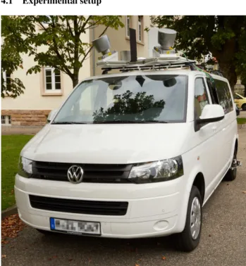
Figure 1. Sensor vehicle used for the experiments.
The data used for the experiments were recorded with a GNSS/-INS augmented sensor vehicle (cf. Figure 1). On this vehicle,
two Velodyne HDL-64E laser scanners are located over the front corners of the vehicle roof, and are positioned on a wedge with a 25 degree angle to the horizontal. This configuration guarantees a good coverage of the roadway in front of the car and allows scanning of building facades alongside and behind it. For direct georeferencing an Applanix POS LV inertial navigation system is built into the van. It comprises the following sensor components: an IMU (inertial measurement unit), two GNSS antennas and a DMI (distance measuring indicator).
Each one of the laser scanners has a rotation rate of 10 Hz and a data rate of approximately 1.3 million points per second. The navigation system has a data rate of 200 Hz.
4.2 Data acquisition
GNSS (e.g., GPS) signals are – among other things – influenced by atmospheric and multipath effects. Within our experiments, we used additional GNSS data of nearby reference stations to reduce the impact of atmospheric effects. This can be done in realtime (RTK) as well as during postprocessing, and it results in a more accurate and precise position estimation. In this pa-per, the inclusion of precise GNSS reference data allowed us to focus on the model generation without having to deal with local-ization and data alignment issues. However, in future work, the presented methods for model generation will be supplemented by simultaneous localization and mapping (SLAM) techniques.
Prior to the actual measurements, the two laser scanners have been calibrated by a procedure presented in (Gordon and Mei-dow, 2013) to achieve best possible precise point measurements. The transformation between the coordinate systems of the two scanners was determined by using the ICP algorithm (Besl and McKay, 1992). The relative orientation and position of the laser scanners with respect to the navigation system was calculated by using the approach presented in (Levinson and Thrun, 2010). For each single laser range measurement, the position and orienta-tion of the vehicle was calculated by linear interpolaorienta-tion from the 200 Hz navigational data.
4.3 Test site
Figure 2. Aerial view of the test site1
The data acquisition took place at a small test site, which is the outside area around our institute building, partly shown in Fig-ure 2. The main part of the scene is a big building surrounded by neighboring structures and some trees. The path driven dur-ing the measurements is shown in Figure 3. The data acquisition took about 2.5 minutes and resulted in approximately 250 mil-lion 3D points. This value is smaller than the actual data rate of 1Ettlingen, Fraunhofer Institut IOSB by Wolkenkratzer http://
commons.wikimedia.org/wiki/File:Ettlingen,_Fraunhofer_
Institut_IOSB.JPG under http://creativecommons.org/
the laser scanners, since some points measured in close vicinity of the sensors (e.g., the vehicle roof) were filtered out during the point generation process.
Figure 3. Path driven by the sensor vehicle during the data ac-quisition (Image data: Google Earth, Image c2014 GeoBasis-DE/BKG).
A part of the measured points is shown in Figure 4.
Figure 4. Plotted accumulated 3D data after reduction to a voxel grid (for visualization).
5. RESULTS AND DISCUSSION
The previous section described the experimental setup and the ac-quisition of data used for the experiments. We carried out differ-ent runs of the algorithms with these data to investigate, analyze and validate our approach. In each run one of three parameters was altered. For the other parameters a default value was set. Ta-ble 1 lists the default values for all parameters. The evaluated three parameters are theallowed distance, theproportion of
out-liersand theminimal variation. The reconstruction error is not
considered for the evaluation, because it is directly linked to the
allowed distance-parameter, which is an upper bound for the
re-construction error.
parameter value
allowed distance 0.25 m proportion of outliers 0.2
RANSAC iterations 100 minimal cell size 0.1 m
kstart 50
kmax 201 minimal variation 0.2
test delay 10 scans Table 1. Default values for the parameters.
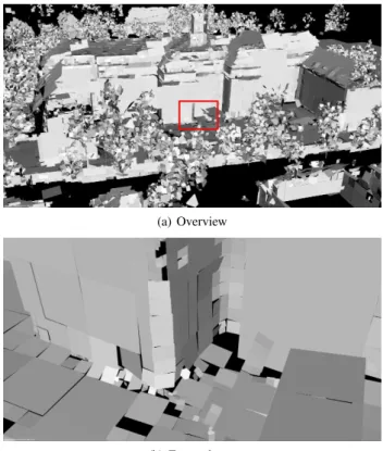
Figure 5(a) shows a part of the polygon model (without the re-maining single points), which resulted from applying our method
with the default parameter settings to the acquired data set. It is visualized from the same viewpoint as Figure 4. Most of the polygons have a quadratic shape. After applying our approach, the surface of the model is not continuous, because there typi-cally is a small gap between neighboring polygons. Especially the trees lead to many small and unconnected polygons, which have a nearly random orientation.
(a) Overview
(b) Zoomed area
Figure 5. Polygon model generated with the default parameter settings. The content of the area marked in Figure (a) is shown zoomed in by Figure (b).
5.1 Variation of theallowed distance
In the first experiment the allowed point-to-plane distance was altered in the range from 1 cm to 100 m. The resulting space sav-ings are shown in Figure 6. Here the termspace savingsmeans the proportion of saved data to the original amount of data and is calculated with equation (1). Throughout this paper, the terms
space savingsandcompression rateare used synonymously.
s= 1−#points mesh+ ##C+ #points in cells w. p.
points (1)
In Figure 6 the abscissa is plotted with a logarithmic scale. The compression rate obviously increases up to 90% until anallowed
distanceof 0.1 m. For higher values the compression rate keeps
nearly stable, between anallowed distanceof 0.5 m and 100 m there is only little change.
The point handling (cf. Algorithm 1) and the test for uniform distribution (cf. section 3.3) are the most time consuming parts. Therefore the calculation of the intersection between octree cells and their associated planes is excluded from the runtime assess-ment. Figure 7 depicts the measured runtimes. The graph shows a nearly opposite behavior when compared to that of the data com-pression rate: First the runtime clearly decreases until anallowed
0 0.1 0.2 0.3 0.4 0.5 0.6 0.7 0.8 0.9 1
0.01 0.1 1 10 100
sp
ac
e
savings
allowed distance [m]
Figure 6. Resulting space savings for different allowed point-to-plane distances.
0 2000 4000 6000 8000 10000 12000
0.01 0.1 1 10 100
[s]
allowed distance [m]
Figure 7. Runtime for differentallowed distances.
stable runtime values. The plotted time for anallowed distance of 0.01 m equals to approximately 3 hours, followed by 18 min-utes for 0.25 m and 5 minmin-utes for 100 m. However, these values are specific to our (still not optimal) implementation, the methods are appropriate to run in realtime on an operational system.
The results show a close relation between computation time and data compression rate. The reason for the high computation time in case of small values for theallowed distanceis the frequent need for plane fitting and octree cell division. With a higher bound, the points can simply be added to existing planes. This reduces the number of octree cells without plane and therefore results in better compression rates. However, this also leads to a higher loss of details. In an extreme case (e.g.,allowed distance of 100 m) nearly all points of the data set are represented by only one plane, which of course is not the desired result.
If the scene contains a lot of planes, the precision and accuracy of the point positioning have a significant influence on the compres-sion rate, given a certainallowed distance. If theallowed distance is too small, most measured 3D points remain untouched and the compression rate is poor. In our case, the precision and accuracy of the point positioning process are in a combined magnitude of approximately 20 cm.
For the following experiments a tradeoff between space savings, runtime behavior and level of detail is needed. We decided to set
theallowed distanceto 0.25 m for all other experiments.
5.2 Variation of theproportion of outliers
For the second experiment, the maximum allowedproportion of
outlierswas varied between 1% and 90%.
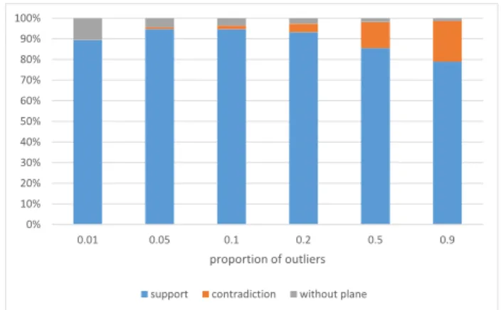
The resulting proportion of the different point sets is shown in Figure 8. If a cell contains a plane, the number of points in each
0% 10% 20% 30% 40% 50% 60% 70% 80% 90% 100%
0.01 0.05 0.1 0.2 0.5 0.9
proportion of outliers
support contradiction without plane
Figure 8. Proportion of the different point sets.
set (support set, contradiction set) is counted. In case of an octree cell without plane, its number of points increases the “without plane” counter. The average proportion of support sets is an in-dicator for the possible space savings, since the associated points are supposed to be represented by planes.
In the case of only one percent of allowed outliers, there are vir-tually no outliers and over 10 percent of the points lie in cells without plane. On the other hand, with 90 percent allowed out-liers, there are (on an average) about 20 percent outliers and only very little points in cells without plane. With the data used in our experiments, the optimum value of the average support set size was reached with aproportion of outliersof 5 percent.
0 500 1000 1500 2000 2500
0 0.2 0.4 0.6 0.8 1
[s]
proportion of outliers
Figure 9. Runtime for differentproportions of outliers.
Obviously there is a negative correlation between runtime and the setting of theproportion of outliers(cf. Figure 9). The curve has a higher slope between 1% and 20%proportion of outliers and a smaller slope between 20% and 90%. The runtime in our experiments varied between 35 minutes and 10 minutes.
The compression rate decreases with higher outlier rate, since the outlying points represent 3D details in the scene and only the support set points can be replaced by planes. If the space savings and the runtimes are compared, theproportion of outliershas a higher influence on the runtime. It decreases from 35 minutes to 9 minutes, which is a reduction of 75%. The compression rate only shows a reduction of 15%.
5.3 Changing parameter setting ofminimal variation
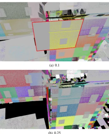
in red with points only on70%of its right side. In Figure 10(b) this big polygon is missing and its area is instead represented by smaller ones, which are nearly totally filled with points. In addi-tion, there are areas where no polygon was assigned to the points. These areas are shown as black parts in Figure 10(b). An excep-tion are the window areas of the building facades, that are covered by polygons. Presumably these areas are too small and only have a minor impact on the standard deviations (cf. subsection 3.3). In summary, with a higher value for theminimal variationthe point variation test reduces the cell size down to its minimal allowed setting, so that the points are nearly spread over the whole plane or polygon, respectively.
(a) 0.1
(b) 0.25
Figure 10. Parts of the polygon models and the points in the sup-port sets (thinned for visualization) for differentminimal
varia-tions(points of the same cell have the same color).
6. CONCLUSIONS AND FUTURE WORK
We have presented an approach for adaptive and fast surface re-construction based on MLS data acquired in urban areas. It takes points as input and tries to represent them by planes, which results in a lossy but efficient data compression. Especially the influence of the two parametersallowed distanceand proportion of
out-lierswas analyzed. Both parameters have an important influence
on the computation time. The data compression rate is influenced by both, but theallowed distanceshowed a more important influ-ence. In combination with the minimal allowed cell size, these parameters control the level of detail of the resulting (polygon) model. This allows the usage for the intended application: The polygon model can be rendered in real-time and therefore allows the inspection e.g. by emergency services. The compression rate of more than 90% enables an easier and faster transmission.
Future work will focus on different areas: Vegetation in the scene results in many small and randomly orientated polygons (cf. sec-tion 4.). A better representasec-tion could consist of thinned points which are marked as vegetation. In some cases the possibility of cell fusion could gain better space savings. The implementation
of the approach needs to be optimized. In this context, we plan to implement parts of the algorithms (e.g., the test of uniform distri-bution) to run on multiple CPUs. Texturing the model with RGB data will be an additional extension.
We will supplement the 3D model generation with realtime 3D-SLAM techniques, which will especially be useful for indoor ap-plications where no GNSS-signals are available. Even in the out-door case, we observed inaccurate GNSS data due to multipath effects. So we expect to clearly benefit from SLAM techniques even in that case, which will result in a better model accuracy and precision.
References
Besl, P. and McKay, N. D., 1992. A method for registration of 3-D shapes. IEEE Transactions on Pattern Analysis and Machine Intel-ligence 14(2), pp. 239–256.
Fischler, M. A. and Bolles, R. C., 1981. Random sample consensus: a paradigm for model fitting with applications to image analysis and automated cartography. Communications of the ACM 24, pp. 381– 395.
Gordon, M. and Meidow, J., 2013. Calibration of a multi-beam Laser System by using a TLS-generated Reference. ISPRS Annals of Pho-togrammetry, Remote Sensing and Spatial Information Sciences II-5/W2, pp. 85–90.
Hansen, W. v., Michaelsen, E. and Th¨onnessen, U., 2006. Cluster Anal-ysis and Priority Sorting in Huge Point Clouds for Building Recon-struction. In: 18th International Conference on Pattern Recognition (ICPR’06), pp. 23–26.
Hoppe, H., DeRose, T., Duchamp, T., McDonald, J. and Stuetzle, W., 1992. Surface Reconstruction from Unorganized Points. In: Pro-ceedings of the 19th Annual Conference on Computer Graphics and Interactive Techniques, SIGGRAPH ’92, ACM, pp. 71–78.
Jo, Y., Jang, H., Kim, Y.-H., Cho, J.-K., Moradi, H. and Han, J., 2013. Memory-efficient real-time map building using octree of planes and points. Advanced Robotics 27(4), pp. 301–308.
Levinson, J. and Thrun, S., 2010. Unsupervised calibration for multi-beam lasers. In: International Symposium on Experimental Robotics.
Lorensen, W. E. and Cline, H. E., 1987. Marching Cubes: A High Reso-lution 3D Surface Construction Algorithm. In: Proceedings of the 14th Annual Conference on Computer Graphics and Interactive Techniques, SIGGRAPH ’87, ACM, pp. 163–169.
Marton, Z. C., Rusu, R. B. and Beetz, M., 2009. On Fast Surface Re-construction Methods for Large and Noisy Datasets. In: IEEE Inter-national Conference on Robotics and Automation (ICRA), pp. 3218– 3223.
Remondino, F., 2003. From point cloud to surface: the modeling and visualization problem. International Archives of Photogrammetry, Re-mote Sensing and Spatial Information Sciences 34(5), pp. W10.
Rusu, R. B. and Cousins, S., 2011. 3D is here: Point Cloud Library (PCL). In: IEEE International Conference on Robotics and Automa-tion (ICRA), Shanghai, China, pp. 1–4.
Vaskevicius, N., Birk, A., Pathak, K. and Poppinga, J., 2007. Fast detec-tion of polygons in 3d point clouds from noise-prone range sensors. In: Safety, Security and Rescue Robotics, 2007. SSRR 2007. IEEE International Workshop on, pp. 1–6.
Vosselman, G., Gorte, B. G. H., Sithole, G. and Rabbani, T., 2004. Recog-nising structure in laser scanner point clouds. International Archives of Photogrammetry, Remote Sensing and Spatial Information Sciences 46(8), pp. 33–38.