Energy Efficient Smartphone-based Users Activity Classification

(1)

F

ACULDADE DE

E

NGENHARIA DA

U

NIVERSIDADE DO

P

ORTO

Energy Efficient Smartphone-based

Users Activity Classification

Ricardo Manuel Correia Magalhães

Mestrado Integrado em Engenharia Informática e Computação Supervisor: João Manuel Paiva Cardoso

(2)

(3)

Energy Efficient Smartphone-based Users Activity

Classification

Ricardo Manuel Correia Magalhães

(4)

(5)

Abstract

With the advance of technology, most people carry a smartphone with built-in sensors (e.g., GPS, accelerometer, gyroscope, light) capable of providing useful data for Human Activity Recogni-tion (HAR). A number of machine learning classificaRecogni-tion methods were already researched and developed for HAR systems, each with different accuracy and performance. HAR systems can be applied to areas such as health, by helping monitor people, entertainment, by suggesting TV shows, or advertisement.

Capturing data from sensors and executing machine learning classifiers requires computational power. As such, factors like inadequate preprocessing can have a negative impact on the overall HAR performance, even on high-end handheld devices. While high accuracy can be extremely important in some applications, the device’s battery life can be highly critical to the end-user.

In this dissertation, we study some of the most used mobile and real-time HAR methods in order to understand their energy consumption impact when considering a number of activities (e.g., "running", "walking", "driving"). This study also allows us to understand trade-offs between accuracy levels and energy consumption savings. Then, we focus on the k-nearest neighbors algorithm (k-NN), one of the most used algorithms in HAR systems, and research and develop energy-efficient implementations for mobile devices.

We propose a valid alternative k-NN implementation based on LSH with a significant posi-tive impact on the device’s battery life, fully integrated into a mobile HAR Android application executing classification in real-time.

Keywords: Human activity recognition (HAR), mobile sensors, machine learning, mobile appli-cation, context-aware applications

(6)

(7)

Resumo

Com o avanço da tecnologia, a maioria das pessoas levam consigo um smartphone com sensores embutidos (e.g., GPS, acelerómetro, giroscópio, luz) capazes de fornecer dados úteis para re-conhecimento de atividade humana (tradução livre de Human Activity Recognition (HAR)). Um número de métodos de classificação em machine learning já foram investigados e desenvolvido para sistemas de HAR, cada um com diferentes níveis de exatidão e desempenho. Os sistemas HAR podem ser aplicadas em áreas como saúde, ajudando na monitorização de pessoas, entreten-imento, ao sugerir programas de televisão, ou publicidade.

Capturar dados dos sensores e executurar classificadores baseados em técnicas de aprendiza-gem máquina requer poder computacional. Assim, factores como pré-processamento inadequado podem levar a um impacto negativo no desempenho global de sistemas HAR, mesmo em smart-phones topo de gama. Embora a alta exatidão seja extremamente importante em algumas apli-cações, o tempo de utilização do dispositivo sem recarregar a bateria pode ser altamente crítica para o utilizador final.

Nesta dissertação, estudamos alguns dos métodos HAR mais usados para dispositivos móveis e em tempo-real, de forma a perceber o seu consumo energético quando considerado um número de actividades (e.g. "correr", "andar, "conduzir"). Este estudo permite também perceber o com-promisso entre níveis de exatidão e redução de consumo energético. Focamo-nos no algoritmo k-Nearest Neighbours(k-NN), um dos algoritmos mais usados em sistemas HAR, investigando e desenvolvendo uma implementação eficientemente energética para aparelhos móveis.

Propômos uma alternativa válida de implementação de k-NN baseada em LSH com um im-pacto positivo significativo no desempenho da bateria do aparelho sem recarregar, completamente integrado numa aplicação HAR em Android que classifica em tempo real.

Palavras-chave: Human activity recognition (HAR), mobile sensors, machine learning, mobile application, context-aware applications

(8)

(9)

Acknowledgements

This work has been partially funded by the European Regional Development Fund (ERDF) through the Operational Programme for Competitiveness and Internationalisation - COMPETE 2020 Pro-gramme and by National Funds through the Portuguese funding agency, Fundação para a Ciência e a Tecnologia (FCT) within project POCI-01-0145-FEDER-016883.

This dissertation could not be achieved without the support of many individuals. First, I would like to thank my supervisors, João Cardoso and João Moreira, for all the guidance throughout this dissertation. Also, I would like to thank Paulo Ferreira for our work and research together.

I am also grateful for my family, specially my parents José Magalhães and Glória Magalhães, for all the encouragement and support needed all these years, letting me pursue my dreams.

I also thank my girlfriend, Susana Gomes, for all the love, care and always being proud and believing in me.

Last, but not least, my gratitude to all friends and colleagues who, in one way or another, crossed paths with me in a positive way.

(10)

(11)

“I used to work in a factory and I was really happy because I could daydream all day.”

(12)

(13)

List of Figures

2.1 Machine Learning Categories . . . 6

2.2 HAR general steps . . . 7

2.3 Possible dummy decision tree in HAR . . . 8

2.4 Probabilistic Approximate Window algorithm in pseudocode, Source: [BPRH13, p. 3] . . . 9

2.5 Adaptive Windowing algorithm in pseudocode, Source: [BG07, p. 2] . . . 10

3.1 Architecture diagram for the desktop application . . . 16

3.2 Architecture diagram for the Android application . . . 17

4.1 Train and test time for k-NN, NB, HT and Ensemble . . . 21

4.2 Training time with different window sizes for each k-NN approach . . . 24

4.3 Testing time with different window sizes for each k-NN approach . . . 24

4.4 Training and testing time with different overlap values . . . 26

4.5 Testing time with different k values . . . 28

4.6 Training time with different frequencies . . . 31

(16)

(17)

List of Tables

1.1 Survey on management of features to increase battery life (survey sample = 748),

Source: [HFT+16, p. 7] . . . 2

1.2 Battery life and power consumption (Nokia N95), Source: [BPH09, p. 1] . . . . 2

3.1 Data collection details . . . 14

3.2 Sensors used for collecting data . . . 14

3.3 Features extracted from 1D sensors . . . 14

3.4 Features extracted from 3d sensors . . . 15

4.1 PAMAP2 testing datasets performance . . . 20

4.2 Performance comparison of k-Nearest Neighbours, Naive Bayes, Hoeffding Tree and Ensemble . . . 21

4.3 Number of training and testing windows for different window sizes . . . 22

4.4 Perfomance of each k-NN approach with different window sizes . . . 23

4.5 k-NN Accuracy per Activity with different Window Sizes . . . 23

4.6 k-NN performance with different overlap values . . . 26

4.7 k-NN Accuracy per Activity with different overlap values . . . 27

4.8 k-NN performance with different k values . . . 28

4.9 k-NN Accuracy per Activity with different k values . . . 28

4.10 LSH k-NN performance with different number of hash tables (l) with hk = 1 . . . 29

4.11 LSH k-NN perfomance with different number of projections per hash value (hk) . 30 4.12 LSH k-NN performance with different sampling frequencies . . . 31

4.13 Dataset perfomance with k-NN and LSH k-NN with different frequencies . . . . 33

(18)

(19)

Abbreviations

API Application Programming Interface IMU Inertial Measurement Unit

GPS Global Positioning System HAR Human Activity Recognition LSH Locally-sensitive Hashing OS Operating System

SDK System Development Kit SVM Support Vector Machine

(20)

(21)

Chapter 1

Introduction

Human Activity Recognition’s (HAR) [LL13] main purpose resides on recognizing activities per-formed by individuals in a certain context, playing a key alliance with ubiquitous or pervasive computing.

Possibly, this area began with computer vision, mainly by analyzing sequences of images and analyzing its visual features [AC99]. By 2001, there were already conclusive experiments with real-time activity recognition [DD01]. With the advent of smartphones, people started to carry around a computing device with integrated sensors, opening an opportunity to use these devices for HAR. While computer vision approaches are good for security [SLMR02] or motion-tracking applications, its main concerns are the privacy and the impossibility of having a camera around tracking every moment in one’s daily life and requring more computational power, thus consuming more energy from the device’s battery.

1.1 Motivation

As mentioned above, we live in a world were most people carry around a smartphone or another wearable with built-in sensors (e.g., GPS, accelerometer, gyroscope). These sensors are capable of gathering useful data for HAR and the use of Machine Learning classifiers has already been studied to recognize activities.

The accuracy of these activities can be useful in certain areas already explored, such as health, particularly monitoring elder people [ÁSÁGA17] or maintaing an healthy lifestyle [LML+11]. There is also the potential of giving contextualized recommendations to the user, such as sug-gesting TV shows, places to visit, physical activity to perform or even improve advertisements by correlating different data results. Also, in an age where social networking is mostly omnipresent on everyone’s lives, this opened the possibility of giving automatic personal information on activ-ities to one’s social circle [SCF+10].

(22)

2 Introduction

1.2 Problem

With the increase of computing power in smartphones, battery’s life are always one of the main concerns by the users. A survey among Portuguese youth individuals [HFT+16] reveals around 30% of the sample population is always managing mobile features or capabilities in order to in-crease the daily battery life (see Table1.1).

Frequency % Always 30.7 Very frequently 22.8 Frequently 18.6 Not frequently 12.1 Rarely 7.4 Never 8.4

Table 1.1: Survey on management of features to increase battery life (survey sample = 748), Source: [HFT+16, p. 7]

Therefore, one of the main concerns with mobile HAR is its energy efficiency. Capturing data from sensors requires constant background tasks. Battery life and power consumption tests were performed on a Nokia N95 device, concluding some sensors should only be used when appropriate [BPH09]. Table1.2shows the battery’s life and power consumption resultant from the use of specific smartphone sensors.

Sensor Approximate battery life (hrs) Average power consumption (mW)

Video camera 3.5 1258 IEEE 802.11 6.7 661 GPS (outdoors) 7.1 623 GPS (indoors) 11.6 383 Microphone 13.6 329 Bluetooth 21.0 211 Accelerometer 45.9 96

All sensors turned off 170.6 26

Table 1.2: Battery life and power consumption (Nokia N95), Source: [BPH09, p. 1]

While accelerometer presents itself as the sensor with the less impact (considering the sensors analyzed in [BPH09]), it has a considerable impact when none of the sensors are used, having only ≈ 27% of the original battery life. However, it should be noted that this does not take in account the personal usage of the mobile device. The implementation of such an HAR application with usage on other services, as mentioned before, can not lead to an overall negative impact on energy efficiency. Therefore, the energy consumption must be minimal.

(23)

1.3 Goals and Contributions 3

1.3 Goals and Contributions

This study aims to contribute to the HAR scientific community, in a initial phase, by studying a number of classifiers and their overall energy efficiency. After that, a mobile prototype (using a smartphone) shall be developed and proposed based on k-NN, achieving a good balance of accuracy versus energy efficiency.

1.4 Dissertation Structure

We conclude the introduction by presenting the structure of our dissertation and the goal of each chapter. This dissertations consists of five different chapters, briefly explained below.

Chapter2summarizes the background needed in order to understand different aspects of HAR, namely smartphone sensors, machine learning techniques and the tools needed in order to imple-ment our solution. This chapter concludes with a summary of different studies regarding our specific problem, energy consumption in HAR.

Chapter3presents a summary of our metholodogies, including some details on the implemen-tation and investigation.

Chapter 4shows all our HAR studies and experiments, including a description, results and conclusions for each experiment.

Chapter5presents our final conclusions about our studies and suggestions for further research on this area.

(24)

(25)

Chapter 2

Background and State-of-the-Art

This chapter aims to summarize the different topics related to our study. Fist, we focus on de-scribing the different smartphone sensors, machine learning approaches and tools used. Finally, an overview of similar studies is presented.

2.1 Smartphone Sensors

First, we focus on the most used smartphone sensors and their general use and main goal, summa-rized as follows:

• Accelerometer: responsible for measuring acceleration, typically in 3-axis (x, y, z). It is suited for motion detection in space, like running and walking.

• Gyroscope: responsible for measuring rotation in 3-axis. (x, y, z). Its main goal is to detect the phone’s orientation in the same space.

• Magnetometer: responsible for measuring magnetic fields, capable of identifying the di-rection of North.

• GPS: responsible for connecting to multiple satellites around the globe, giving the map coordinates (latitude and longitude) of the localization of the user/device. It is suited for navigation applications and/or applications requiring the localization of the user.

• Barometer: responsible for measuring air pressure. It is suited for detecting weather changes.

• Proximity: responsible for detecting proximity with the aid of an infrared LED and light detector. It is suited for turning off the screen when near the ear (calling) or facing down on a surface.

(26)

6 Background and State-of-the-Art

• Ambient light sensor: responsible for detecting the ambient light in a place. It is suited for auto-adjusting screen brightness or for identifying light conditions of the environment where the user is located.

• Microphone: responsible for recording and detecting sound in the area.

There are other sensors (e.g., temperature or light sensor) available. However, they are not widely present in every smartphone.

2.2 Machine Learning

Machine Learning [Mit97] is a field in Computer Science responsible for applying methods and algorithms to help the machine "learn" from data. ML techniques can be organized in different categories, based on the labeling of data (see Figure2.1).

Figure 2.1: Machine Learning Categories

Supervised learning centers on having pre-labeled data with inputs associated with desired outputs, known as training data, using classification or regression. Unsupervised learning, on the other hand, uses unlabeled data and can be approached by clustering or association. Semi-supervised learning is a mix of the latter two, presenting both labeled or unlabeled data, as some-times labeling all data may be unfeasible and there is advantages in having some unlabeled data present [LL13].

On HAR, evaluation can be online or offline. When the solution is implemented online, im-mediate real-time response is given, being particularly useful for healthcare continous monitoring or gaming. By contrary, offline is approached when there’s no need for real-time response, as in analyzing diet or exercising habits. Supervised learning can be both offline or online, while unsupervised tends to be implemented offline [LL13].

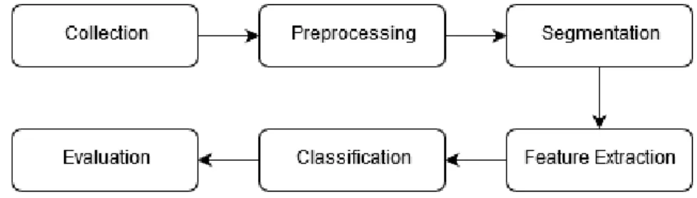
2.2.1 HAR Steps

Most HAR solutions present the set of steps [BBS14] [SBI+15] illustrated in Figure2.2.1. The following list provides a summary of these steps:

(27)

2.3 HAR Classifiers 7

Figure 2.2: HAR general steps

1. Data collection: specific sensor data is collected, normally with supervision and following a set of rules.

2. Data preprocessing: transform and filter the data. Sometimes a sensor data calibration phase is performed [LSN+18].

3. Data segmentation: identify segments which like contain information about an activity, based on the processed data. Several techniques exist, such as sliding window [KC14]. 4. Feature extraction: reduce the segmented data into features, giving the possibility to

in-crease accuracy and reduce response time [LN15], using three different domains: time do-main, frequency domain and discrete representation domain [FDFC10]. While a large num-ber of features can increase accuracy, it also requires a higher computation. Features used by other researches can be categorized into magnitude-based features, frequency-based fea-tures, correlation feafea-tures, among others [FFN+12].

5. Classification: train classifiers and classify activities.

6. Evaluation: evaluate the accuracy and performance of the classification done in the earlier phase.

2.3 HAR Classifiers

Classification is usually a learning method where the solutions learns from the input data and then classifies new data. There have been many ML-based classifiers applied to HAR, described in the following subsections, such as k-Nearest Neighbors [CH67], Naive Bayes [Ris99], Support Vector Machines [CV95] and Decision Trees [McS99].

2.3.1 Naive Bayes

Based on Bayes’ theorem, Naive Bayes classifiers [Ris99] are one the most known, being studied since the 1950s. One of the main assumptions of these classifiers is the independence between features, even if some are correlated or dependent on each other. Therefore, this might present a

(28)

One of the main advantages of Naive Bayes is its lightness and only needing a small amount of data to output results.

2.3.2 Decision Trees

Decision trees [McS99] build an hierarchical tree using a divide-and-conquer strategy, consisting of dividing the problem in a number of subproblems. These decision trees are represented with decision and leaf nodes being mapped to attributes and values, respectively.

Decision trees are easily understandable to non-experts, as they can be graphically represented. It requires less data preparation and it is suited for large datasets, acheving better speed results and less computation cost when compared to other classifiers [LLS98]. Also, they mirror human decision making.

Figure 2.3: Possible dummy decision tree in HAR

2.3.3 k-Nearest Neighbors

k-Nearest Neighbors [CH67], or k-NN, is one of the simplest classifiers. It works by choosing the ktraining instances in the feature space and by classifying a new instance by a majority vote of its neighbors, where k is the number of neighbors it checks.

The choice of k is dependent on the data. While larger values reduce noise on classification, boundaries between classes might become less distinct.

Being a lazy learner, the function is approximated locally, delaying the generalization of the data until a query is made. Therefore, there is not an explicit training phase, keeping all training data during the classification phase. While it can solve simultaneous problems, this can be a problem when presented with a large training dataset, because of the computation required to calculate all distances. It can also evaluate more slowly in relation to other classifiers by suffering from long execution times to classify [Bha10].

(29)

2.3 HAR Classifiers 9

However, there are a number of studies on different alternatives to improve k-NN, trying to solve its high storage and computation [Ang05]. One such approach consists of data reduction techniques with prototype selection or generation [GDCH12] [TDGH12]. Clustered k-NN was shown to significantly reduce CPU usage [KIE12], being more suited to be used online [US15], while still achieving high accuracy.

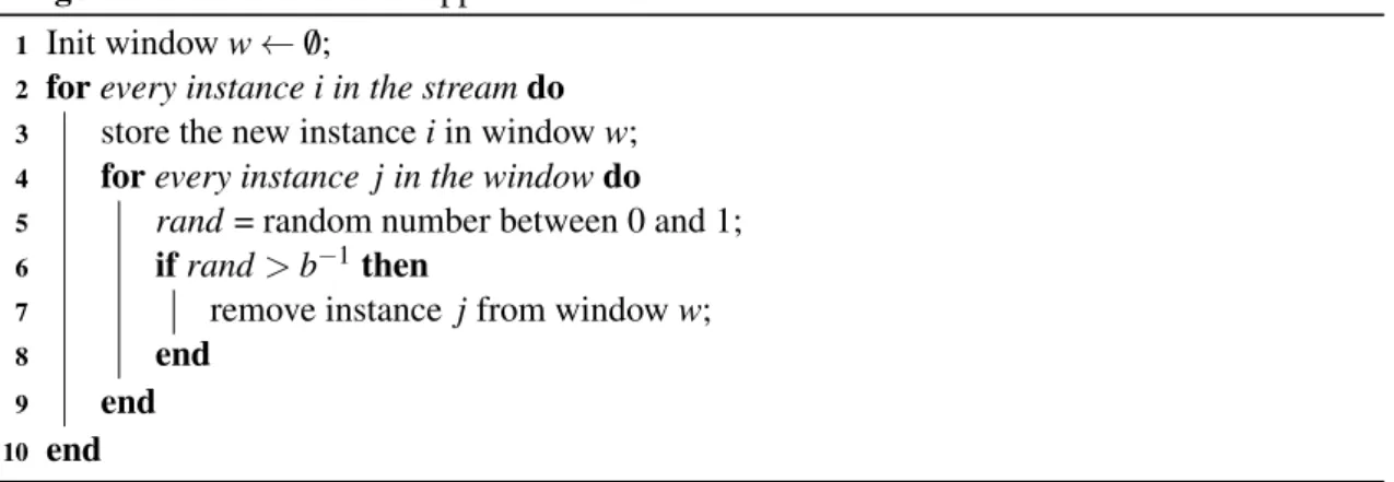
2.3.4 k-NN with PAW & ADWIN

Among other alternatives to improve k-NN’s performance, we select two that were designed to reduce the number of windows stored by the classifier.

Probabilistic Adaptive Window (PAW) [BPRH13] maintains in logarithmic memory a sample of the windows, storing the most recent with an higher probability. When a new vector of features is stored for training, this algorithm iterates each one and applies a randomized removal with a probability of 1 − b−1, where b = 2−1/w as proposed by Flajolet [Fla85]. Figure2.4 presents PAW’s algorithm in pseudocode.

Algorithm 1: Probabilistic Approximate Window

1 Init window w ← /0;

2 for every instance i in the stream do 3 store the new instance i in window w;

4 for every instance j in the window do 5 rand= random number between 0 and 1; 6 if rand > b−1then

7 remove instance j from window w;

8 end

9 end

10 end

Figure 2.4: Probabilistic Approximate Window algorithm in pseudocode, Source: [BPRH13, p. 3]

Adaptive Windowing (ADWIN) [BG07] works by discarding old windows whenever two "large enough" subsets present "distinct enough" averages by concluding the expected values are different. It can be combined with PAW [BPRH13].

2.3.5 Approximate Nearest Neighbor

In order to save memory and improve speed, an Approximate Nearest Neighbor approach can be used with k-d trees [Ota13]. In those cases, the actual nearest neighbor is not guaranteed, but presents an high probability.

Another interesting technique is Locality-sensitive Hashing (LSH) [SC08], using dot products with random vectors to find the neighbor more quickly. There are also other studies proposing new algorithms that exploit the same approximation LSH does [LMGY04], while exploring different

(30)

10 Background and State-of-the-Art Algorithm 2: ADWIN 1 Init window W ← /0; 2 for each t > 0 do 3 W← W ∪ {xt}; 4 repeat

5 drop elements from the tail of W ;

6 until | ¯µWo− ¯µW1| ≥ εcut holds for every split of W into W = W0·W1; 7 output ¯µW

8 end

Figure 2.5: Adaptive Windowing algorithm in pseudocode, Source: [BG07, p. 2]

2.3.6 Support Vector Machine

Support Vector Machine [CV95], or SVM, is another classification approach in HAR. It centers on the construction a hyperplane in a high or infinite-dimensional space.

SVMs work well when the number of dimensions is greater than the number of instances. Also, it is memory efficient. However, a large dataset might impact negatively the time required to train the model.

2.3.7 Ensemble Learning

Ensemble learning [Die02] characterizes on combining outputs of different classifiers in order to improve accuracy. Typically, a number of classifiers is applied and a majority voting scheme is used to select a classification. Some of those techniques include bagging, boosting or stack-ing. However, these kind of approaches improves accuracy with the cost of a higher computation required [LL13].

2.4 Tools

This section aims to summarize the tools, OS and libraries worth mentioning in order to achieve our goals.

2.4.1 Android

HAR systems can be implemented on a number of different of mobile operating systems. While the first and earlier studies focused on Symbian, Android took over as the main system target [SBI+15]. Therefore, we focus our efforts and tests on an Android smartphone.

Android is an open-source mobile operating system launched by Google in 2008, based on a Linux kernel. It became the best-selling and most widely used mobile OS. Android applications are mainly developed in Java with the aid of Android SDK, extensively documented and with a huge number of tutorials, namely on activity recognition [Goo].

(31)

2.5 Related Work 11

Regarding energy consumption, Android’s API on regular cellphones just presents an update of the energy level, which says little information [CGSS13]. While this could provide some valid estimations, alternatives such as using ODROID’s1current/voltage sensors or connecting a multi-meter2to the actual smartphone could give more accurate measurements.

2.4.2 MOA

MOA (Massive Online Analysis) [BHKP10] is a popular framework for implementing machine learning algorithms from data streams, providing a GUI and command-line for making experi-ments. Being written in Java, it provides a powerful API capable of running in Android applica-tions. Therefore, this framework serves as our main interaction with machine learning algorithms.

2.4.3 Smile

Smile (Statistical Machine Intelligence and Learning Engine) [LSN+18] is a framework for ma-chine learning, covering every aspect of it, while delivering state-of-the-art performance. This framework is mainly used on our work because of its LSH implementation.

2.5 Related Work

After presenting background information in topics surrounding HAR and Machine Learning, we will now explore and present a number of studies and implementations focused on mobile HAR with the aim of energy saving.

Yan et al. [YSC+12] proposed a new strategy, A3R (Adaptive Accelerometer-based Activity Recognition, based on investigation of effects in sampling frequency and classification features. This study claims this approach can reduce energy consumption by 50% under ideal conditions, while users running on their Android device save between 20% to 25%.

Zheng et al. [ZWR+17] developed a system based on H-SVM and experimented with different sampling rates, concluding that the energy consumption is considerably lower when adopting a lower sampling rate. Adopting a rate of 1 Hmz saves 59.6% power than of 50 Hz. One interesting example comes from the difference between 10 Hz to 50Hz, where the later only increases 0.03% accuracy from the former but increases energy consumption by 32.7%.

Wang et al. [WLA+09] propose EEMSS, capable of characterizing a user’s state by time, location and activity, while exploring sensor monitoring by only keeping the minimum sensors, triggering new ones when state transition is recognized. Tests performed on a Nokia N95, powered with Symbian, provided an average accuracy of 92.56% with an average battery lifetime of 11.33 hours, depending on the user activity.

(32)

Liang et al. [LZYG14] propose a hierarchical recognition solution with decision trees based on recognition of 11 activities with only accelerometer data, reducing energy consumption with lower sampling rates and increasing accuracy with adjusts to the size of sliding window.

Anguita et al. [AGO+13b] explored three different types of SVM algorithms, concluding L1-SVM is capable of achieving high accuracy with less computation by performing dimensionality reduction. Also, the impact of adding gyroscope features improved accuracy results.

Anguita et. al [AGO+13a] explore the use of fixed-point arithmetic in energy savings, propos-ing a modified SVM. It was found the battery lifetime with 32-bit integer averages to 119 hours, while a 32-bit float averages to 89 hours, saving up to 25%.

Morillo et al. [MGARdlC15] proposes the use of discrete variables obtained from accele-moteres sensors, applying the Ameva algorithm. While saving up to 27 hours of usage time, it maintains an average accuracy of 98% with 8 activities.

2.6 Summary

Many different techniques, methods and approaches have been used for energy-saving HAR sys-tems [PTTHGZ16] or HAR in general [AGSK15] [LL12] [SBI+15] [UIE13]. Those techniques range from preprocessing techniques to classifier algorithms optimization, each having its advan-tages and disadvanadvan-tages. However, it must be noted that there is a lack of studies around the use of k-NN with LSH for reducing energy consumption.

(33)

Chapter 3

Methodological Approach

This chapter summarizes the work done throughout this dissertation, including key methodologies for achieving our final results.

3.1 Dataset and Data Collecting

The first step in HAR studies is to identify an existing dataset and/or collect our own data. As a matter of fact, inadequate datasets can negatively impact HAR performance [Car16]. In order to gather more data, sometimes it is not possible to replicate the original conditions with different individuals.

3.1.1 PAMAP2

We first started using PAMAP2 (Physical Activity Monitoring for Aging People) [RS12], a dataset where 18 different activities were recorded with 9 different subjects, each wearing 3 IMUs (Inertial Measurement Units) and a heart-rate monitor. Over 10 hours of data are presented, with each IMU presenting 3D-data from accelerometer, gyroscope and magnetometer. More specifically, 3850505 data samples are present on the dataset.

3.1.2 Our Own Dataset

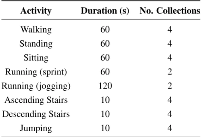
The CONTEXTWA project [CMV18] further addressed more activities over the ones already present on PAMAP2, totaling the number of activities to 66 (see AppendixA). For further data collection, we used an Android-based Samsung Galaxy J5 to collect data from 9 different sensors (see Table3.2) for 8 different activities (see Table3.1for further details). Each activity was col-lected using a sampling frequency of 5 Hz with the device located on the pant’s right pocket, being upside down and with the screen facing the leg of the user.

(34)

14 Methodological Approach

Table 3.1: Data collection details

Activity Duration (s) No. Collections

Walking 60 4 Standing 60 4 Sitting 60 4 Running (sprint) 60 2 Running (jogging) 120 2 Ascending Stairs 10 4 Descending Stairs 10 4 Jumping 10 4

Table 3.2: Sensors used for collecting data Sensor Dimension Accelerometer 3 Game Rotation 3 Gravity 3 Gyroscope 3 Proximity 1 Linear Acceleration 3 Rotation 3 Magnetic Field 3 Light 1

3.2 Feature Extraction

For both datasets, a number of features were extracted using measures such as mean, correlation and standard deviation. Each 1D and 3D sensor has, respectively, 2 and 10 features extracted. In total, each window consisted of 45 extracted features for PAMAP2 and 74 for our own dataset. Tables3.3and3.4present a detailed list of all features extracted for each sensor.

Table 3.3: Features extracted from 1D sensors 1D Sensor Features

Mean Standard Deviation

(35)

3.3 Environment 15

Table 3.4: Features extracted from 3d sensors 3D Sensor Features xMean yMean zMean Mean xStandard Deviation yStandard Deviation zStandard Deviation xyCorrelation xzCorrelation yzCorrelation

3.3 Environment

During this study, we worked on two different environments. For most studies, we worked offline with Eclipse IDE for Java development. As Android is our OS of choice, our main working environment for developing our application was Android Studio, Google’s official IDE for its platform.

As mentioned on Chapter2, the frameworks MOA [BHKP10] and Smile [LSN+18] were the libraries for working with machine learning techniques and classifiers.

3.4 Architecture

Since our studies were conducted on two different environments, we present both architectures in this section and give a summary of each one.

3.4.1 Offline Java Application

Our offline Java application is responsible for doing all our offline ML studies. Figure3.1 illus-trates its architecture.

This application is capable of converting CSV (Comma-separated Values) files to ARFF (Attribute-Relation File Format), which is then loaded by MOA to store all data instances. Then, it is capable of extracting all features, respecting window size and overlap values, and create a feature vector (or window) to be used as training or testing in the classifier. Finally, we are able to run our classifiers independently or with an ensemble of our choice, executing the testing phase on the

(36)

16 Methodological Approach sensor-acc.csv sensor-gam.csv sensor-gra.csv sensor-gyr.csv sensor-lig.csv sensor-lin.csv sensor-mag.csv sensor-pro.csv sensor-rot.csv train_set.arff test_set.arff CSV to ARFF Feature Extraction Feature Extraction Feature Vector Feature Vector Ensemble Classiﬁer Predictive Model Classiﬁcation kNN Naive Bayes Hoeffding Trees LSH kNN with PAW & ADWIN kNN with PAW

Figure 3.1: Architecture diagram for the desktop application

3.4.2 Android Application

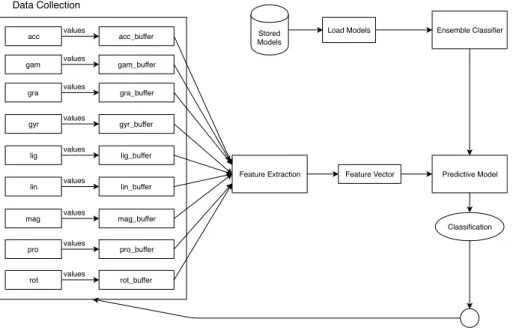
Our Android application is responsible for doing all our online ML studies. Figure3.2illustrates its architecture.

This application is capable of collecting data from sensors in order to create a dataset or to be stored in different buffers in order to be used on live classification. For the latter,it basically collects data until all buffers are full (i.e., window size is reached), extracting all features to create a vector to be tested on the classifier, cleaning the buffer afterwards. The classifiers are loaded by models created on the desktop application, already containing the trained dataset. Finally, the application notifies the classified activity to the user.

3.5 Energy Studies and Optimization

Our first goal was to test and compare the impact of different classifiers, namely k-NN, Naïve Bayes and Decision Trees. This was helpful in order to get a first insight in these algorithms performances.

We then shifted our focus to NN. We first studied different alternative approaches, namely k-NN with PAW (Probabilistic Approximate Window) and k-k-NN with PAW and ADWIN (Adapative Windowing) [BPRH13], while also exploring different window sizes and overlap values. We also studied the variation between k values.

After that, we studied LSH k-NN [AI06] [DIIM04] perfomance, mainly with different vari-ables, such as number of projections per hash value (hk), number of hash tables (l) and the width of the projection (r).

(37)

3.6 Summary 17

acc values acc_buffer

gam values gam_buffer

gra values gra_buffer

gyr values gyr_buffer

lig values lig_buffer

lin values lin_buffer

mag values mag_buffer

pro values pro_buffer

rot values rot_buffer

Feature Extraction Feature Vector Predictive Model

Data Collection

Classiﬁcation Stored

Models

Load Models Ensemble Classiﬁer

Figure 3.2: Architecture diagram for the Android application

We also reduced the PAMAP2 dataset to different frequencies in order to understand the trade-off between energy-saving and accuracy.

Finally, we ran live HAR tests using our Android application in order to understand the impact on battery usage.

3.6 Summary

This chapter presented an explanation of the investigation methodologies in order to solve our problem. We chose to focus our study on optimizing k-NN’s performance and by incorporating LSH in order to reduce energy consumption, as the latter was not yet explored in this area and could present itself a valid approach for a less resource-hungry classifier applied to smartphone

(38)

(39)

Chapter 4

HAR Energy Studies and Experiments

This chapter covers all studies and experiments performed throughout this dissertation, including a brief summary, results and conclusions.

4.1 Offline Studies

Most of the studies in this section were conducted with the PAMAP2 [RS12] dataset already presented in Chapter 3 in order to evaluate the performance of different classifiers and finding optimalarguments for this particular case. After these studies, we analyzed the performance on our own dataset.

All experiments done on this section were made on an Acer Aspire F 15 (5-572G-556R) laptop with an Intel Core i5-6200U (2.3 GHz) processor, an NVIDIA GeForce 940M (4GB dedicated) graphics card and 8GB DDR3 of RAM, and with an Ubuntu-based Linux distribution (elementary OS 0.4.1 Loki).

4.1.1 PAMAP2 User Study

Description

The PAMAP2 dataset was collected using 9 different subjects. Therefore, while every instance in the dataset is used on the training phase, our experiments could be tested against 9 different testing datasets representative of each subject’s collections. The strategy for training and testing is leaving each tested user’s data out of the training phase.

A study was made by testing each user’s data and comparing the global accuracy of each one. For testing purposes, each experiment was conducted with the same conditions (window size = 250; overlap = 10%; k = 3) using the k-NN classifier.

(40)

20 HAR Energy Studies and Experiments

Results

In this section, we present the total number of windows with the specified window size and the global accuracy taking every activity into account.

Table 4.1: PAMAP2 testing datasets performance Subject Total Windows Global Accuracy

1 1110 66.31% 2 1170 81.62% 3 774 86.18% 4 1028 86.09% 5 1210 72.40% 6 1111 80.20% 7 1034 86.65% 8 1164 51.37% 9 28 35.71% Conclusions

Out of 9 different experiments, 5 present satisfactory and similar results, while the other ones suffer from a lower accuracy. Taking this study into account, data collected from subject 7 presented the best global accuracy. As such, all the following experiments were conducted with this subject’s dataset for the testing phase.

4.1.2 k-NN, Naive Bayes and Hoeffding Tree

Description

This study’s purpose was to test the base k-NN implementation present on MOA against other two ML classifiers (Naive Bayes and Hoeffding Tree), in order to sustain our early option to focus on optimizing k-NN.

Each experiment was conducted in the same conditions for each of the three classifiers (win-dow size= 250; overlap = 10%).

Results

In this section, we present a comparison of four classifiers (k-Nearest Neighbours, Naive Bayes, Hoeffding Tree and Ensemble of the previous three) in terms of global accuracy and both training and testing time.

(41)

4.1 Offline Studies 21

Table 4.2: Performance comparison of k-Nearest Neighbours, Naive Bayes, Hoeffding Tree and Ensemble

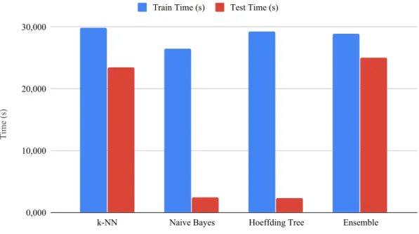
Classifier Training Time (s) Testing Time (s) Global Accuracy (%)

k-NN 29.874 23.532 86.65 Naive Bayes 26.430 2.455 88.68 Hoeffding Tree 29.292 2.392 88.68 Ensemble 29.000 25.048 88.78 Classifier Time (s) 0,000 10,000 20,000 30,000

k-NN Naive Bayes Hoeffding Tree Ensemble Train Time (s) Test Time (s)

Figure 4.1: Train and test time for k-NN, NB, HT and Ensemble

Conclusions

The results show that the three classifiers behave similarly in predicting the activities on the testing dataset. However, k-NN presents a much bigger computational cost by taking approximately 10 times longer than the other two classifiers to test the dataset. The ensemble suffers from the same problem because of the k-NN.

Therefore, the base k-NN implemented in MOA is not a suited classifier for this particular case with a large dataset. As it was expected in the beginning of this study, alternative implementations

(42)

4.1.3 Alternative k-NN Approaches and Window Size Variation

Description

As it was concluded on the last experiment, the base k-NN is not suited for this case. How-ever, we selected two different alternative approaches to k-NN present on MOA: k-NN with PAW (Probabilistic Approximate Window) and k-NN with PAW and ADWIN (Adaptive Windowing), described in Chapter2.

This study’s goal was to compare base k-NN with the other alternative implementations in terms of global accuracy and both training and testing time with different window sizes. Since PAMAP2 was recorded in 100 Hz, each 100 instances represent 1 second in time. Therefore, we chose to experiment with increments of 100 in window size.

Each experiment was conducted in the same conditions for each of the three classifiers (k = 3; overlap= 10%).

Results

In this section, we first show the number of training and testing windows for different window sizes in Table 4.3. Table 4.4 shows our results with different window sizes for each classifier. Table4.5shows a detailed accuracy for each activity on base k-NN for window size ≥ 500.

Table 4.3: Number of training and testing windows for different window sizes

Window Size k-NN k-NN with PAW k-NN with PAW+ADWIN Training Windows Testing Windows Training Windows Testing Windows Training Windows Testing Windows 100 19000 2586 18665 2586 1179 2586 200 9500 1293 9471 1293 1975 1293 300 6333 862 6319 862 5171 862 400 4750 646 4744 646 2636 646 500 3800 517 3796 517 3796 517 600 3166 430 3163 430 3163 430 700 2714 369 2712 369 2712 369 800 2375 323 2373 323 2373 323 900 2111 287 2109 287 2109 287 1000 1899 258 1898 258 1898 258

(43)

Table 4.4: Perfomance of each k-NN approach with different window sizes

Classifier 100 200

Train (s)

Test (s)

Window Avg. Test (s) Global Acc. (%) Train (s) Test (s)

Window Avg. Test (s) Global Acc. (%) k-NN 28.541 124.521 0.047 78.73 29.393 36.969 0.024 83.45 k-NN with PAW 36.403 135.53 0.047 78.69 31.321 37.811 0.024 83.45 k-NN with PAW+ADWIN 76.152 10.888 0.03 41.22 57.439 8.399 0.04 73.16 Classifier 300 400 Train (s) Test (s)

Window Avg. Test (s) Global Acc. (%) k-NN 26.866 17.964 0.019 87.35 3.,497 12.945 0.013 88.24 k-NN with PAW 31.845 21.038 0.019 87.24 27.446 11.436 0.013 87.24 k-NN with PAW+ADWIN 59.296 14.042 0.013 87.12 46.984 7.649 0.007 85.60 Classifier 500 600 Train (s) Test (s)

Window Avg. Test (s) Global Acc. (%) k-NN 26.550 8.231 0.010 89.75 26.989 6.144 0.010 90.93 k-NN with PAW 26.338 7.960 0,011 89.75 29.727 6.570 0.010 90.93 k-NN with PAW+ADWIN 39.102 7.580 0.010 89.75 38.385 6.839 0.009 90.93 Classifier 700 800 Train (s) Test (s)

Window Avg. Test (s) Global Acc. (%) k-NN 26.953 5.821 0.009 89.16 31.967 4.933 0.007 91.95 k-NN with PAW 28.828 5.376 0.009 89.16 29.389 5.275 0.007 91.95 k-NN with PAW+ADWIN 35.479 5.126 0.008 89.16 35.373 4.673 0.007 91.95 Classifier 900 1000 Train (s) Test (s)

Window Avg. Test (s) Global Acc. (%) k-NN 27.708 4.199 0.006 93.38 28.598 3.700 0.006 92.64 k-NN with PAW 28.160 4.061 0.006 93.38 29.507 3.826 0.006 92.64 k-NN with PAW+ADWIN 31.909 3.903 0.006 93.38 32.448 4.033 0.005 92.64

Table 4.5: k-NN Accuracy per Activity with different Window Sizes

Window Size Accuracy (%)

All Lying Sitting Standing Walking Running Cycling Nordic

Walking Asc. Stairs Desc. Stairs Vacuum Cleaning Ironing 500 89.75 98.25 92.59 98.25 90.67 75 92 96.88 82.05 76.92 79.17 83.33 600 90.93 97.87 95.65 93.75 91.93 66.67 90.48 98.11 81.81 77.27 80 94.44 700 89.16 95.12 94.73 95.12 88.89 80 88.89 95.65 85.71 83.33 82.35 80.85 800 91.95 97.22 88.24 97.14 91.49 80 96.77 97.50 91.67 76.47 83.33 90.24

(44)

24 HAR Energy Studies and Experiments Window Size Train time (s) 0 20 40 60 80 200 400 600 800 1000

k-NN k-NN with PAW k-NN with PAW+ADWIN

Figure 4.2: Training time with different window sizes for each k-NN approach

Window Size Train time (s) 0 20 40 60 80 200 400 600 800 1000

k-NN k-NN with PAW k-NN with PAW+ADWIN

(45)

Conclusions

This study made several conclusions possible in regards to the three classifiers and different win-dow sizes, both in its accuracy and time.

As it can be seen, and as expected, the three classifiers take less time to classify all samples when the window size increases. However, neither one of the alternative approaches really out-performs the base k-NN in training and testing time or the global accuracy. k-NN with PAW consistently present similar training and testing time in relation to k-NN; sometimes, one takes longer than the other, which can be explained by conditions on the system not being the same ev-ery time the experiment takes place. On the other hand, k-NN with PAW and ADWIN started by taking significantly less time to complete classification with a negative impact on global accuracy because of discarding many samples. However, as the window size increases, this approach starts to discard less samples, until it reaches a point where it discards the same as k-NN with PAW only. The three classifiers behave similarly when window sizes are of 500 or more instances, achiev-ing the same global accuracy in each experiment. When windows consist of 900 instances (i.e., each window represent 9 seconds of activity), the maximum global accuracy of 93.38% is reached, taking 4 ± 0.1 seconds to classify all samples.

4.1.4 Overlap Study

Description

This study’s goal was to test different values of overlap from 0% to near 100%, in order to evaluate the global accuracy and computational cost.

The overlapping technique consists of maintaining a percentage of all samples considered in the current window, transitioning to the next one. Exemplifying, if an overlap of 10% is applied to a window size consisting of 100 samples of data, the last 10 will be considered first on the next window. This is particularly important in HAR because activities can span different times and are not instantly changed (i.e., a person who is running will not instantly stop that activity). Therefore, the transition between activities is important to this case.

Each experiment was conducted in the same conditions for base k-NN (window size = 900; k = 3). Since k-NN with PAW and k-NN with PAW and ADWIN did not improve the overall performance for this dataset, it did not seem relevant to perform further tests using those classifiers.

Results

In this section, we first present Table4.6 with k-NN performance with different values overlap, showing the training and testing time. Following, we present more detailed results with accuracy

(46)

Table 4.6: k-NN performance with different overlap values Overlap (%) Windows Train Time (s) Test Time (s) Global Acc. (%) 0 1900 28.007 3.847 92.25 10 2111 27.675 3.965 93.38 20 2374 28.264 4.423 94.12 30 2714 26.962 5.750 92.95 40 3166 31.122 6.617 93.72 50 3799 29.749 8.485 93.80 60 4761 30.614 11.894 94.27 70 6331 32.247 20.564 94.30 80 9549 36.651 43.696 94.44 90 18992 42.513 135.635 94.41 Overlap (%) Time (s) 0,000 50,000 100,000 150,000 0 20 40 60 80

Train Time (s) Test Time (s)

(47)

Table 4.7: k-NN Accuracy per Activity with different overlap values

Overlap Accuracy (%)

Walking Asc. Stairs Desc. Stairs Vacuum Cleaning Ironing 0 92.25 96.43 92.86 93.10 91.90 100 88.46 96.88 85 84.62 83.33 100 10 93.38 100 93.33 96.88 100 75 96.43 97.22 95.24 73.33 77.78 91.67 20 94.12 100 88.89 97.14 96.37 80 96.77 97.50 100 82.35 83.33 95.12 30 92.95 100 85 92.68 90.74 66.67 94.44 100 92.86 88.89 88.24 93.62 40 93.72 100 93.75 90.48 83.33 95.24 100 93.75 93.75 81.82 87.50 96.30 50 93.80 100 92.86 100 89.33 85.71 90.20 98.44 87.50 92.00 85.42 98.46 60 94.27 98.59 97.06 97.22 93.62 77.78 93.65 98.75 93.75 84.85 85 96.34 70 94.30 100 97.78 97.92 90.40 75 94.05 99.06 92.19 84.09 86.25 98.17 80 94.44 100 94.20 99.41 91.01 77.78 92.91 99.38 91.84 87.69 87.60 96.95 90 94.41 100 93.43 98.95 90.40 77.78 94.05 99.38 92.35 90.70 86.67 96.33 Conclusions

As expected, testing time increases progressively as the overlap reaches 90%, which is justified by the increase in the number of windows to be classified. Even if the best overall global accuracy is achieved with a 80% overlap, this is not feasible because of its testing time of 43.696 seconds.

In order to get a better trade-off between accuracy and computation cost, the choice lies with 10% and 20% overlap. However, while the latter performs relatively better accuracy-wise, we opted to perform the next experiments with 10% overlap because it takes approximately 0.5 sec-onds less to classify all samples, even with a less accuracy of 0.74%.

4.1.5 Impact of k Value

Description

One of the particularities of k-NN is the value of k. If k = 1, then the class is simply assigned to the class of its nearest neighbour. Therefore, it is expected that the testing time will increase with bigger values of k. This study’s goal is to choose the best value in relation to accuracy and testing time.

Each experiment was conducted in the same conditions (window size = 900; overlap = 10%).

Results

(48)

Table 4.8: k-NN performance with different k values k Value Train Time

(s) Test Time (s) Global Acc. (%) 1 27.210 3.804 93.73 2 26.785 3.940 93.38 3 26.595 3.929 93.38 4 27.021 4.123 94.08 5 30.346 4.734 92.33 k Value Test Time (s) 3,500 3,750 4,000 4,250 4,500 4,750 1 2 3 4 5

Figure 4.5: Testing time with different k values

Table 4.9: k-NN Accuracy per Activity with different k values

k Value Accuracy (%)

Walking Asc. Stairs Desc. Stairs Vacuum Cleaning Ironing 1 93.73 100 93.33 100 95.12 75 96.43 97.22 95.24 80 77.78 94.44 2 93.38 100 93.33 96.88 100 75 96.43 97.22 90.48 73.33 81.48 91.67 3 93.38 100 93.33 96.88 100 75 96.43 97.22 95.24 73.33 77.78 91.67 4 94.08 100 93.33 93.75 100 75 96.43 97.22 95.24 80 81.48 94.44 5 92.33 96.88 86.67 96.88 95.12 75 96.43 97.22 95.24 73.33 77.77 94.44

(49)

Conclusions

By evaluating different possible k values for k-NN, we can conclude that 1-NN is a valid option for this particular dataset, taking 3.804 seconds to classify all samples with an accuracy of 93.73%.

4.1.6 k-NN Optimization with LSH

Description

In order to further optimize the k-NN classifier, the LSH (Locality Sensitive Hashing) was our choice. Because MOA [BHKP10] lacks a LSH [LSN+18] implementation, we used the Smile library. Therefore, our k-NN with LSH implementation consists of combining Smile’s LSH inside MOA’s base k-NN, basically creating a wrapper between the two.

LSH presents three main parameters with an impact of performance: number of projections per hash value (hk), number of hash tables (l) and the width of the projection (r). Since our last study concluded k = 1 is sufficient for this dataset, that value is used. For hk, we tested values from 1 to 3. Regarding the width of the projection, the authors suggest the value to be sufficiently away from 0 [DIIM04], but not too large because of an increase in query time; in this particular dataset, r= 10 was considered optimal because it is the smaller value with biggest accuracy, since r > 10 does not improve accuracy anymore and increases the query time. Our last parameter to test was l, which we tested from 10 to 60.

Our goal is to find an optimal value of l and hk, maintaining a good trade-off between time and accuracy.

Each experiment was conducted in the same conditions (window size = 900; overlap = 10%, k = 1, r = 10).

Results

In this section, we present the results of LSH k-NN performance with both different l and hk by training and testing time and accuracy. As most testing windows take less than 1 ms to test, we did not calculate the average.

Table 4.10: LSH k-NN performance with different number of hash tables (l) with hk = 1

l Train time (s) Test Time (s) Accuracy (%)

All Lying Sitting Standing Walking Running Cycling Nordic Walking Asc. Stairs Desc. Stairs Vacuum Cleaning Ironing 1 26.654 2.222 78.40 93.75 93.33 96.88 95.12 50 92.86 61.11 42.86 33.34 44.44 97.22 5 27.609 2.247 88.50 96.88 93.33 100 100 75 96.43 97.22 61.90 60.00 48.15 100 10 27.744 2.354 89.90 96.88 100 100 100 75 96.43 97.22 71.43 53.33 55.56 100 20 26.67 2.483 90.24 100 100 100 100 75 96.43 97.22 71.43 53.33 55.56 100 30 27.911 2.779 90.24 100 100 100 100 75 96.43 97.22 71.43 46.67 59.26 100 40 28.959 2.561 90.24 100 100 100 100 75 96.43 97.22 71.43 46.67 59.26 100

(50)

Table 4.11: LSH k-NN perfomance with different number of projections per hash value (hk) hk Train Time (s) Test Time (s) Global Acc. (%)

1 27.857 2.475 90.24 2 28.882 2.614 87.46 3 27.497 2.225 74.22 4 28.764 2.297 46.34 5 30.080 2.215 22.30 Conclusion

From this study, we can conclude that l = 20 can be considered an optimal number for this partic-ular case, achieving the same global accuracy than l > 20 and takes less time to test all samples. Also, we conclude hk = 1 presents the best global accuracy.

We also conclude that activities like ascending stairs or descending stairs are easily mistaken with the other, specially descending stairs. The activity running suffered from having less samples on the testing dataset; with a window size = 900, there are only 4 testing windows representing running and one is mistaken for nordic walking.

Finally, we can also notice how LSH k-NN with l = 20 took ≈ 35% less time to test all windows compared to base k-NN, while just losing 3.49% of accuracy.

4.1.7 Sampling Frequency Study

Description

As mentioned in Chapter 2, the sampling frequency which data is captured can have an impact on the classifier’s performance [ZWR+17]. Logically, reducing the frequency will result in less computation. The goal of this experiment is to study if reducing sampling frequency will result in a good trade-off between performance and accuracy.

Since PAMAP2 was recorded using a sampling frequency of 100 Hz (i.e., data was recorded each 10 ms), we applied a filter to its data in order to progressively reduce the frequency, deleting some of the instances.

Each experiment was conducted in the same conditions (overlap = 10%, k = 1, r = 10, l = 20) with the LSH k-NN classifier. Since our optimal window size for 100 Hz is 900 (i.e., 9 seconds), this value is reduced to still represent the same time span (e.g., for 50 Hz, window size = 450). As such, the number of training and testing windows always stays the same (2111 and 287, respectively).

(51)

Results

Table4.12shows LSH k-NN performance with different sampling frequencies, showing the train-ing and testtrain-ing time, as well as accuracy per activity. Figures4.6and4.7present results for training and testing time.

Table 4.12: LSH k-NN performance with different sampling frequencies

f (Hz) Train time (s) Test Time (s) Accuracy (%)

Walking Asc. Stairs Desc. Stairs Vacuum Cleaning Ironing 100 26.67 2.483 90.24 100 100 100 100 75 96.43 97.22 71.43 53.33 55.56 100 50 14.781 1.396 90.94 100 100 100 100 75 96.43 97.22 71.43 60 59.26 100 25 7.532 0.948 90.94 96.88 100 100 95.24 50 100 100 77.27 71.423 55.56 100 5 1.964 0.692 89.31 96.88 93.33 96.88 100 50 100 97.22 81.82 66.66 44.44 97.30 1 0.861 0.645 85.52 96.88 93.33 100 92.86 75 96.43 80.56 65.22 50 55.55 97.30 Frequency (Hz) Time (s) 0 10 20 30 20 40 60 80 100

(52)

32 HAR Energy Studies and Experiments Frequency (Hz) Time (s) 0 0,5 1 1,5 2 2,5 20 40 60 80 100

Figure 4.7: Testing time with different frequencies

Conclusions

From this study, we successfully conclude that smaller sampling frequencies are more suited to situations where less computation is needed.

With f = 5 Hz, it took ≈ 93% less time to train the dataset and ≈ 72% less time to test all samples, while just losing 0.93% of accuracy. Curiously, with f = 50 Hz and f = 25 Hz, the accuracy actually improved by 0.7%.

Another interesting conclusion is the bigger accuracy some activities get on reduced frequen-cies, particularly both ascending stairs and descending stairs. This could be related to some noisy data being eliminated.

4.1.8 Our Own Dataset

Description

As mentioned in Chapter3, we collected data using a sampling frequency of 5 Hz using a Samsung Galaxy J5 (2017) with 9 available sensors from a single user. Data was distinguished in 9 different activities. Each activity collection divides 80% of data for training and 20% to testing. Each window presents 74 different features.

The goal of this study is to support our conclusions in earlier experiments and the performance of LSH k-NN with a different dataset.

(53)

4.2 Online Studies 33

We also performed the experiments in different sampling frequencies. Since our dataset was recorded using a frequency of 5 Hz (i.e., data was recorded each 200 ms), we applied a filter, created for the last study, to its data in order to progressively reduce the sampling frequency.

Each experiment was conducted in the same conditions (overlap = 10%, k = 1, r = 10, l = 20) with k-NN and LSH k-NN classifiers. Similar to the last study, we start with a window size of 45 for 5Hz and reduce it to preserve the same timespan. Therefore, the number of windows (118) stays the same for each one of the experiment.

Results

Table4.13shows k-NN and LSH k-NN performance with our dataset by training and testing time, as well as accuracy per activity.

Table 4.13: Dataset perfomance with k-NN and LSH k-NN with different frequencies

f (Hz) Classifier k = 1 Train time (s) Test Time (s) Accuracy (%) All Walking Standing Desc.

Stairs Asc. Stairs

Running

(Jogging) Sitting Jumping

Running (sprint) 5 k-NN 0.548 0.134 89.66 100 100 0 100 66.67 100 100 100 LSH k-NN 0.527 0.06 96.55 100 100 100 100 100 100 100 50 4 k-NN 0.481 0.081 93.10 100 100 100 100 66.67 100 100 100 LSH k-NN 0.524 0.047 96.55 100 100 100 100 100 100 100 50 2 k-NN 0.399 0.08 89.66 100 100 0 100 66.67 100 100 100 LSH k-NN 0.438 0.042 96.55 100 100 100 100 100 100 100 50 1 k-NN 0.386 0.069 86.21 100 100 0 100 50 100 100 100 LSH k-NN 0.413 0.03 96.55 100 100 100 100 100 100 100 50 Conclusions

From this study, we can observe how LSH k-NN maintains its accuracy on each different fre-quency, while k-NN offers some variations. Also, LSH k-NN presents a better accuracy on every single experiment. However, it should be noted tht k-NN surpasses LSH k-NN on one of the activities, running (sprint).

Focusing on computing perfomance, k-NN is consistently faster on f > 5. However, LSH k-NN spends ≈ 50% less time to test all samples on every experiment.

4.2 Online Studies

This section covers all our online studies using a smartphone. Every experiment was performed on a Samsung Galaxy J5 (2017) with an 64-bit Octa Core Processor (1.6 GHz) and 2 GB of RAM,

(54)

4.2.1 Energy Consumption

Description

In this study, we experimented our application with live recognition on the pocket, while doing daily activities, for 30 minutes and checked how much battery the device had lost. We also detected how much time had spent between each change in battery. For each experiment, the battery started with 100% and the screen remained on with the lowest brightness, while cellular data, Wi-Fi, GPS and Bluetooth were all turned off. We tested both k-NN and LSH k-NN on two different sampling frequencies (5Hz and 1Hz). It should be noted the window size used in both sampling frequencies (45 and 5, respectively) represents a time span of 9 seconds.

The goal of this study is to understand if our proposed LSH k-NN is suited for a live application and the impact of sensor collection on the energy consumed.

Results

Table4.14shows the time span for each change in battery in minutes and seconds. Table 4.14: k-NN and LSH k-NN impact on battery (30 minutes)

Remaining Battery (%)

Time Span (Minutes:Seconds)

5 Hz 1 Hz

k-NN LSH k-NN k-NN LSH k-NN

99 09:20 14:15 09:05 11:05

98 00:18:40 00:25:55 00:18:30 00:23:30

97 N/A N/A 00:28:30 N/A

Conclusions

From this study, we can conclude LSH k-NN spends less energy than k-NN in live activity recog-nition. With 5 Hz, k-NN changes battery state ≈ 6 minutes faster than LSH k-NN.

However, contrary to our predictions, 1 Hz did not spend less energy than 5 Hz. Actually, LSH k-NN gets a worse performance by taking ≈ 3 minutes less to change battery state. While we do not know the reason behind this, we can conclude lowering the sampling frequency which we collect data from sensors does not improve the performance energy-wise.

4.3 Summary

On this chapter, we presented the studies done throughout this dissertation, showing all the results and conclusions. We tried to do all studies on a step-by-step basis, as the results of each experiment contributed to following, culminating on our proposed solution.

(55)

Chapter 5

Conclusions

This chapter covers our final conclusions for all studies done throughout this dissertation, as well as potential future work.

5.1 Final Conclusions

The goal of this dissertation was to propose an efficient alternative k-NN implementation applied to mobile HAR, providing a good trade-off between accuracy and battery consumption. From our empirical studies, several conclusions can be made.

First, by analyzing PAMAP2 different accuracy levels between the 9 different users present on the dataset, it can be concluded two different things: patterns in data can be different between different individuals and the data collection protocol should specify the number of times a certain activity should be collected. Since PAMAP2 user’s data was not strict in relation to samples per activity, some activities suffer from this.

With the selection of the user dataset with more accurate data, we compared classification results between k-NN, Naive Bayes, Hoeffding Tree and an Ensemble between the four. Without being optimized or using optimal values, we concluded that k-NN failed to achieve an acceptable testing time, presenting a big computational cost.

After that initial study, we opted for two different paths for improving k-NN performance: finding optimal values for data segmentation, such as window size and overlap, and testing alter-native k-NN approaches which could potentially decrease the computation needed for training and testing.

For the first route, we performed several empirical studies. We can conclude that window size plays an important role on the classifier’s performance, namely for k-NN. As expected, the bigger the window size, the fastest the testing phase is. For our particular case of HAR, 9 seconds of data (i.e., 900 windows on 100 Hz, 45 windows on 5 Hz, ...) proved to be the best trade-off between accuracy and energy-saving. Another import factor is the overlap value, because human activities

(56)

36 Conclusions

present transitions. Increasing this value leads to more windows, leading to an increase in testing time. Our optimal choice was 10%, leading to an overall high accuracy (93.38%), while presenting an acceptable testing time compared to bigger values. This concludes that data preprocessing and segmentation can impact positively the performance and outcome of ML classifiers for HAR for specific activities.

Regarding the classifier itself, we first began to understand if two different k-NN approaches present on MOA (k-NN with PAW and k-NN with PAW and ADWIN) would improve the per-formance. The latter proved to be faster with window sizes ≤ 400 instances, with an acceptable accuracy. After that, the three different implementations behave similarly, as the two alternative approaches discard very few windows. Therefore, there is no positive influence on performance in this particular case by applying PAW and ADWIN to k-NN. We also concluded 1-NN is sufficient for mobile HAR.

Nevertheless, the combination between k-NN and LSH improved the performance regarding accuracy and computation cost. With the same conditions, LSH k-NN actually took ≈ 35% less time to classify all windows into activities, with the cost of just losing 3.49%. We further extended our LSH studies by reducing the dataset’s frequency. As expected, reducing the frequency con-tributes to a positive impact on computation needed because some instances are eliminated (i.e., if a 100 Hz dataset has 1000 instances, there are only 500 with 50 Hz). However, we conclude that using higher frequencies does not correlate to having bigger accuracies, as 5 Hz and 1 Hz reduce dramatically the training and testing times, while achieving acceptable accuracies for this case (89.31% and 85.52%, respectively). Another particular note is the fact that some activities actually improve on accuracy with lower frequencies.

Finally, after collecting our dataset, we tested both k-NN and LSH k-NN in similar conditions for different frequencies, both offline and online. In our offline studies, we concluded LSH k-NN performed significantly better than k-k-NN, achieving always ≈ 50% less time to classify all windows and more accuracy (96.55%). It should also be noted how reducing the frequency did not impact the accuracy on LSH k-NN at all. Doing an battery consumption analysis on an Android device proved that our proposed LSH k-NN performs better than k-NN on both 5 Hz and 1 Hz, as the first takes always more time to lower the battery, thus saving more energy. However, contrary to what was expected before our experiments, reducing the live data collection to 1 Hz did not reduce the energy spent.

In summary, we have successfully proven that applying LSH to k-NN with optimal window sizes, frequency, k and overlap can be positive for developing an HAR-based mobile application for public usage by reducing the overall computation and energy spent.

5.2 Future Work

While our work is a step towards making HAR-based applications more energy-efficient, there is still a lot of future work that can improve our studies.

(57)

5.3 Final Remarks 37

First and foremost, the dataset is key for improving studies on this area. PAMAP2 is a great contribution to the scientific community and was useful for our studies, but we noticed that users should have the same number of activities performed for more concise results. Our dataset ended being somewhat short and only collected by one user in only one place (a park). Therefore, in the future, we could specify a strict protocol to be performed by different individuals in different places for a bigger period of time, as concluded by other works in the area [Car16].

Improving our Android application could potentially lead to more conclusions and proof-of-concept. Namely, we could work on having a dynamic training dataset adapted for each user by adding the correctly classified windows for following trainings (i.e., ask each user if certain activities were correctly identified).

Another possible work on energy-savings could focus on turning on and off sensors dynam-ically on certain situations. For instance, if the GPS sensor is taken in consideration, it could only be turned on when the user is outdoors. Therefore, a study could be made by analyzing which sensors have more impact on different activities. Another possible experiment could be on implementing dynamic sliding windows, since several activities have different time duration.

Finally, more experiments should have been made regarding energy, namely using ODROID for more complete information.

5.3 Final Remarks

Working on Machine Learning, specifically on HAR, proved to be a good challenge. While other techniques could be studied in order to reduce the energy impact of mobile HAR, our proposed LSH k-NN could be a step in the right direction. With our suggestions on the last section, we hope

(58)

(59)

Appendix A

Dataset

A.1 List of Activities

The following is a list of all considered activities in the CONTEXTWA project. Activities 0-24 are present on PAMAP2, but have been extended with different contexts.

• 7 Nordic walking [1 min.] • 9 watching TV [1 min.]

• 10 computer - work | leisure - table | lap [1 min.]

• 11 car driving [1 min.]

• 12 ascending stairs - outdoor | indoor [10 sec.] • 13 descending stairs - outdoor | indoor [10

sec.]

• 16 vacuum cleaning - house | car [1 min.] • 17 ironing [1 min.]

• 18 folding laundry - outdoor | indoor [30 sec.] • 19 house cleaning [1 min.]

• 20 playing soccer - outdoor | indoor [1 min.] • 24 rope jumping - outdoor | indoor [30 sec.] • 25 jogging - for leisure | for exercise - firm

surface | moderate surface - uphill | downhill | flat - outdoor | indoor [1 min.]

• 26 jumping - outdoor | indoor [10 sec.] • 27 taking elevator up [15 sec.]

• 28 taking elevator down [15 sec.]

• 29 moving - by car | by bus | by train | by sub-way [1 min.]

• 30 brushing teeth [15 sec.]

• 31 eating - outdoor | indoor [15 sec.] • 32 cooking [1 min.]

Energy Efficient Smartphone-based Users Activity Classification

F

E

U

P

Energy Efficient Smartphone-based

Users Activity Classification

Ricardo Manuel Correia Magalhães

Energy Efficient Smartphone-based Users Activity

Classification

Ricardo Manuel Correia Magalhães

Abstract

Resumo

Acknowledgements

Contents

List of Figures

List of Tables

Abbreviations

Chapter 1

Introduction

1.1

Motivation

1.2

Problem

1.3

Goals and Contributions

1.4

Dissertation Structure

Chapter 2

Background and State-of-the-Art

2.1

Smartphone Sensors

2.2

Machine Learning

2.3

HAR Classifiers

2.4

Tools

2.5

Related Work

2.6

Summary

Chapter 3

Methodological Approach

3.1

Dataset and Data Collecting

3.2

Feature Extraction

3.3

Environment

3.4

Architecture

3.5

Energy Studies and Optimization

3.6

Summary

Chapter 4

HAR Energy Studies and Experiments

4.1

Offline Studies

4.2

Online Studies

4.3

Summary

Chapter 5

Conclusions

5.1

Final Conclusions

5.2

Future Work

5.3

Final Remarks

Appendix A

Dataset

A.1

List of Activities