COMPARING GLOBAL LAND COVER DATASETS THROUGH
THE EAGLE MATRIX LAND COVER COMPONENTS FOR
CONTINENTAL PORTUGAL
COMPARING GLOBAL LAND COVER DATASETS THROUGH THE EAGLE
MATRIX LAND COVER COMPONENTS FOR CONTINENTAL PORTUGAL
Dissertation supervised by
Mário Caetano, PhD
Co-Supervised by
Roberto Henriques, PhD
Ignacio Guerrero, PhD
i
ACKNOWLEDGEMENTS
I would like to thank everyone who supported me during the course of this dissertation. I would
like show my special gratitude to my supervisor Prof. Mário Caetano who has always shown
his assistance, support and guidance. I also would like to thank my co-supervisors Roberto
Henriques and Ignacio Guerrero for their comments and guidance.
Special thanks to Pedro Sarmento and Filipe Marcelino for their help and contributions for my
thesis.
I would like to express my appreciation to Marco Painho and all other directors, professors and
Erasmus coordinators for supporting me during the master’s program in any situation.
ii
COMPARING GLOBAL LAND COVER DATASETS
THROUGH THE EAGLE MATRIX LAND COVER
COMPONENTS FOR CONTINENTAL PORTUGAL
ABSTRACT
Global land cover maps play an important role in the understanding of the Earth's
ecosystem dynamic. Several global land cover maps have been produced recently namely,
Global Land Cover Share (GLC-Share) and GlobeLand30. These datasets are very useful
sources of land cover information and potential users and producers are many times interested
in comparing these datasets. However these global land cover maps are produced based on
different techniques and using different classification schemes making their interoperability in
a standardized way a challenge. The Environmental Information and Observation Network
(EIONET) Action Group on Land Monitoring in Europe (EAGLE) concept was developed in
order to translate the differences in the classification schemes into a standardized format which
allows a comparison between class definitions. This is done by elaborating an EAGLE matrix
for each classification scheme, where a bar code is assigned to each class definition that
compose a certain land cover class. Ahlqvist (2005) developed an overlap metric to cope with
semantic uncertainty of geographical concepts, providing this way a measure of how
geographical concepts are more related to each other. In this paper, the comparison of global
land cover datasets is done by translating each land cover legend into the EAGLE bar coding
for the Land Cover Components of the EAGLE matrix. The bar coding values assigned to each
class definition are transformed in a fuzzy function that is used to compute the overlap metric
proposed by Ahlqvist (2005) and overlap matrices between land cover legends are elaborated.
The overlap matrices allow the semantic comparison between the classification schemes of
each global land cover map. The proposed methodology is tested on a case study where the
overlap metric proposed by Ahlqvist (2005) is computed in the comparison of two global land
cover maps for Continental Portugal. The study resulted with the overlap spatial distribution
among the two global land cover maps, Globeland30 and GLC-Share. These results shows that
Globeland30 product overlap with a degree of 77% with GLC-Share product in Continental
iii
KEYWORDS
Semantic Uncertainty;
Fuzzy Comparison;
Map Comparison;
Globeland30
iv
ACRONYMS
EAGLE– EIONET Action Group on Land Monitoring in Europe
EEA– European Environment Agency
EIONET – Environmental Information and Observation Network
ETM+ –Landsat Enhanced Thematic Mapper Plus
FAO – Food and Agriculture Organization
GLC – Global Land Cover
GLCC– Global Land Cover Characterization
GLC-Share –Global Land Cover – Share
IGBP-DIS – The International Geosphere-Biosphere Programme Data and Information System
LCC – Land Cover Components
LCCS– Land Cover Classification System
LCM – Land Cover Map
MMU – Minimum Mapping Unit
MODIS –Moderate Resolution Imaging Spectroradiometer
UMD –University of Maryland
UML – Unified Modeling Language
v
INDEX OF THE TEXT
ACKNOWLEDGEMENTS ... I
ABSTRACT ... II
KEYWORDS ... III
ACRONYMS ... IV
INDEX OF THE TEXT ... V
INDEX OF TABLES ... VI
1. INTRODUCTION... 1
1.1 THEORETICAL FRAMEWORK ... 1
1.2 OBJECTIVES ... 2
1.3 DISSERTATION OUTLINE ... 3
1.4 LITERATURE REVIEW ... 3
2. STUDY AREA AND DATASETS ... 6
2.1 STUDY AREA ... 6
2.2 LAND COVER DATASETS ... 7
3. EAGLE CONCEPT ... 11
3.1 BAR CODE APPROACH ... 13
4. METHODOLOGY ... 14
4.1 DATA PREPROCESSING ... 15
4.2 TRANSLATION OF THE NOMENCLATURES INTO EAGLEMODEL ... 15
4.3 CALCULATION OF THE OVERLAP BETWEEN CLASSES ... 19
4.4 PRODUCTION OF THE UNCERTAINTY MAPS ... 25
5. RESULTS AND DISCUSSION ... 27
5.1 OVERLAP MATRIX ... 27
5.2 AERA COMPARISON ... 29
5.3 OVERLAP MAP ... 31
6. CONCLUSIONS ... 33
7. REFERENCES ... 34
vi
INDEX OF TABLES
Table 1 : GLC-Share Land Cover Legend and Class Definitions ... 8
Table 2 : GlobeLand30 Land Cover Legend and Class Definitions ... 9
Table 3 : Technical specification of the global land cover datasets ... 10
Table 4 : Barcode method value list ... 13
Table 5 : An example of calculation of LCC overlap between attributes ... 21
Table 6 : Calculation of overlap of LCC for Cultivated Land class of Globeland30 product and Tree Covered Areas class of GLC-Share product ... 22
Table 7 : Weights for Artificial Surfaces Class from GLC-Share Product... 23
Table 8 : Weights for Grassland class of GLC-Share product... 24
Table 9 : Weights for Tree Covered Areas Class of GLC-Share Product ... 25
Table 10 : Weights and LCC Overlap Values of Forest and Grassland Classes ... 25
Table 11 : Overlap classes defined for the representation of the semantic overlap. ... 27
Table 12 : Spatial overlap areas between GLC-Share and GlobeLand30 in square Km ... 29
vii
INDEX OF FIGURES
Figure 1 : Illustration of a certain pixel in two different land cover dataset ... 2
Figure 2 : Administrative Boundaries of Portugal ... 6
Figure 3 : Dataset distribution of GLC-Share Product ... 7
Figure 4 : Land cover maps in their original legends ... 10
Figure 5 : Schematic illustration of the EAGLE matrix ... 11
Figure 6: Structure of the Land Cover Component (LCC) of EAGLE Matrix ... 12
Figure 7 : Flowchart of the methodology ... 14
Figure 8 : An example of bar code method ... 16
Figure 9 : EAGLE matrix of Globeland30 product ... 17
Figure 10 : EAGLE matrix of GLC-Share product ... 18
Figure 11 : Transformation of the bar code values into a fuzzy function ... 20
Figure 12 : Production of overlap maps process ... 26
Figure 13 : Overlap matrix between GlobeLand30 legend and GLC-SHARE legend. ... 27
Figure 14 : Overlap map between Globeland30 and GLC-Share products. ... 31
1
1.
INTRODUCTION
Theoretical Framework
Global land cover datasets are vital source of information for variety of disciplines such as
agriculture, forestry and transportation. Several global land cover maps are produced recently
such as Global Land Cover-Share (GLC-Share) and Globeland30. Each of these land cover
datasets are produced by the experts considering the purpose of use. Therefore each of these
maps have some temporal, spatial and thematic in/consistencies (Verburg et al., 2011).
Comparison of these data sets is important for the users to reveal the inconsistencies between
datasets, especially before starting a study on a specific topic using these datasets. (Wu et al.,
2008). Thus, they can have good overview about similarities and differences in datasets and it
will help in decision making for their specific application. On the other hand, comparison of
the maps are important in a producer’s perspective to examine the reasons of disagreements in
products, in order to improve the quality of the future products (Caetano and Araújo, 2006).
Because of the spatial, temporal and thematic differences in datasets, comparison of land cover
products is not straight forward process. Figure 1 illustrates the same pixel in two different land
cover datasets. For example, this pixel is classified as Broad Leaved Forest in the first land
cover map while the same pixel is classified as Mixed Forest in another land cover map. In
this case it cannot be assumed that this pixel has total disagreement. In such a situation,
comparison method should also consider class definitions to avoid wrong interpretations.
Another important point is comparing maps pixel by pixel without using a fuzzy approach,
cannot reveal that the difference between two pixels are caused by spatial disagreement or
semantic confusion between the class definitions (Fritz and See, 2008). It can only provide a
2
Figure 1 : Illustration of a certain pixel in two different land cover dataset
Recently, Arnold et al., (2013) introduced a new concept called “EAGLE” –Environmental Information and Observation Network (EIONET) Action Group on Land Monitoring in
Europe- which can be used as a common framework for different land cover and land use maps.
EAGLE concept allows to decompose classes into atomic features and using these features it
is possible compare the maps, applying a fuzzy comparison approach such as Ahlqvist’s (2005) conceptual overlap approach.
In this dissertation, we provide a methodology to compute degree of overlap between land
cover maps using Ahlqvist’s (2005) fuzzy approach throughout EAGLE concept. The proposed
methodology tested on GlobeLand30 and GLC-Share products. Firstly, two land cover datasets
classification schemes translated to an EAGLE Matrix through the Bar Coding Method and
after computed the semantic overlap between the global land cover datasets using the overlap
metric proposed by Ahlqvist (2005). This allowed to compute the semantic overlap matrix
between the global land cover datasets. Using this overlap matrix, it was possible to associate
an overlap degree to each pixel that resulted from the combination of the global land cover
datasets. This way provided a map, illustrating the spatial distribution of the semantic overlap
among the global land cover datasets.
Objectives
This dissertation aims to provide a methodology allowing a map comparison considering
overall and specific agreement instead of traditional yes/no agreement. Using EAGLE model
and Ahlqvist (2005) approach, semantic comparison of the classes will be possible and it will
3 used by users for a specific application or it can be used for the producers to take measures and
develop new methodologies to improve the datasets.
Dissertation Outline
The rest of the dissertation is organized in the following way. In the next section, introduced a
deep literature review on map comparison approaches. In the Second chapter, data and study
area of this dissertation is described. Third chapter provides a brief explanation of EAGLE
concept and bar code approach. In Fourth chapter methodology steps are explained in detail.
Methodology steps consist of pre-procession of the data, translation of the land cover classes
into EAGLE bar code approach, calculation of the overlap matrix using Ahlqvist’ (2005) approach and production of the overlap maps. The fifth chapter highlights the results and
discussions. The dissertation is concluded in the sixth chapter.
Literature Review
Many researchers are interested in comparison of land cover products and they have different
approaches for map comparison. These approaches can be categorized in two groups (Cheng
et al., 2001, Fritz and See 2008, Hagen 2003);
• Feature based comparison
• Pixel based comparison
Feature based comparison or comparison based on fuzziness of location, is an approach
performed by comparing corresponding features of two maps by considering their topological
relations (or geometric aspects) while in pixel based comparison is performed on a pixel by
pixel basis (Dungan 2006). Interested reader about feature based comparison, should review
Hagen (2003).
Pixel based comparison or comparison based on fuzziness of category is performed by
4 are few different existing approaches in pixel based comparisons. We can categorize these
approaches in four groups (Ahlqvist 2004, Comber et al., 2010, Fritz and See 2008):
1. Translating legends into a common classification scheme
This method requires translating classes into a common, bridging classification scheme. Land
Cover Classification System (LCCS) provided by Food and Agriculture Organization (FAO)
is one of the most used classification system for the harmonization of different nomenclatures
of different land cover maps into the same scheme (Congalton, et al., 2005). Many researches
applied this approach with slight differences. Recently, Kuenzer et al., (2014) compared 6
different land cover datasets by using LCCS as a common classification scheme to point out
similarities and differences between products focusing on the Mekong Basin. Similarly, Herold
et al., (2008) compared 4 global land cover maps, The International Geosphere-Biosphere
Programme Data and Information System (IGBP DISCover), University of Maryland (UMD),
Moderate Resolution Imaging Spectroradiometer (MODIS) 1-km and Global Land Cover 2000
(GLC2000), by translating legends into LCCS in order to reveal strengths and weaknesses of
the datasets.
2. Using simplified legends
This approach is performed by collapsing the legends of the datasets into a common, simplified
legend defined by the researcher, mostly depending on the focus of research purpose. Bay et
al., (2014) compared 5 global land cover datasets, namely Global Land Cover Characterization
(GLCC), UMD, GLC2000, MODIS and GlobCover. The classification schemes of the datasets
consist of 17,14,23,17 and 22 classes, respectively. Comparison is performed by collapsing
classification schemes of the 5 different land cover map into 12 common, simplified classes.
Ran et al., (2010), compared IGBP DISCover, MODIS, GLC2000 and land cover product of
UMD by collapsing classification schemes into 7 classes simplified legend. Cabral et al.,
(2010), analyzed land cover datasets produced during the period 1990-2000 to highlight the
changes in certain classes. To compare the datasets they aggregated legends into the five
common, simplified classes depending on the research focus, in their case: Forests,
5 The disadvantage of using simplified legends methodology is that, some information is lost
due to the differences in definition of classes in land cover datasets. For example Cabral et al.,
(2000), decided to define Forest as a class with tree coverage more than 40% in his new
simplified legend. However one of the legends defines forest class as greater than 60% tree
cover, while other legend defines the same class greater than tree coverage percentages
changing between greater than 30% and greater than 60%. Combining these two different
classes into one class lead losing some information.
3. Using expert knowledge:
This approach requires using the knowledge of the experts who produced the land cover data
sets. Fritz and See (2005) used an approach based on expert knowledge. They compared GLC
2000 and MODIS datasets in order to figure out where the differences between two dataset
occur and what is the degree of agreement/disagreement. They conducted a survey for experts
consisting of questions about how difficult to differentiate classes from each other. The survey
questions are answered in a scale from very easy to very difficult. The answers of the surveys
are used to create agreement/disagreement maps on a pixel base. To cope with the differences
in legends between datasets they created a look up table which makes the approach independent
of legend definitions. Similarly, Comber et al., (2004), used experts` opinion in order to cope
with the difficulties in detecting the change between two land cover datasets (LCM 1990 and
LCM2000).
4. Using conceptual overlaps:
Ahlqvist (2005) provided a fuzzy approach to calculate the degree of overlap. By calculating
the degree of conceptual overlap, the disagreement caused by inconsistency in the class
definitions, can be revealed. Fritz and See (2008) compared two land cover datasets (GLC 2000
and MODIS) considering user specific applications. In their work, additionally, they used a
questionnaire answered by user to define the importance of disagreement between classes.
When comparing the maps they created a legend lookup table which is allowing one to many
6 approach. Similarly Perez-Hoyoz et al., (2012) compared four land cover maps (Corine,
GLC2000, MODIS and Globcover) using conceptual overlaps approach. Firstly they translated
legends into LCCS by a software provided by FAO. Later they calculated overlap metric with
an approach similar to Ahlqvist’s (2005) approach.
2.
STUDY AREA AND DATASETS
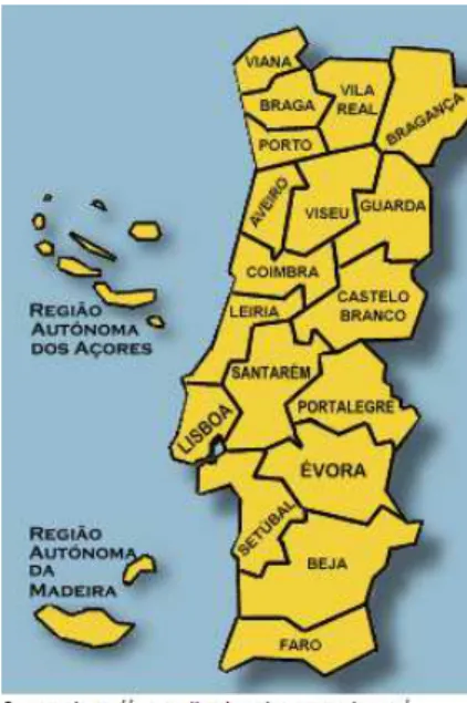
Study Area
Portugal is a country located on the west of Iberian Peninsula with population of 10,562,178
and with a total area of 92,212 km2 (Ine.pt, 2016). The main climates of Portugal are
Mediterranean, Mixed Oceanic and Semi-arid climate (Weatheronline.co.uk, 2016). Portugal
is bordered by Spain to the east and north, Atlantic Ocean to the west and the south. Portugal
consist of 18 districts and two autonomous islands namely Madeira and Azores (Figure 2).
Study area excludes the islands and includes only Continental Portugal.
7
2.2 Land Cover Datasets
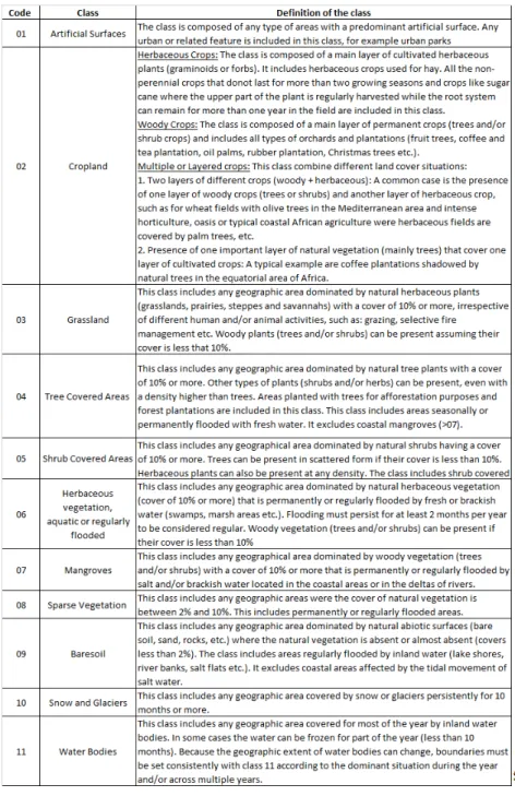
2.2.1 Global Land Cover-Share Product
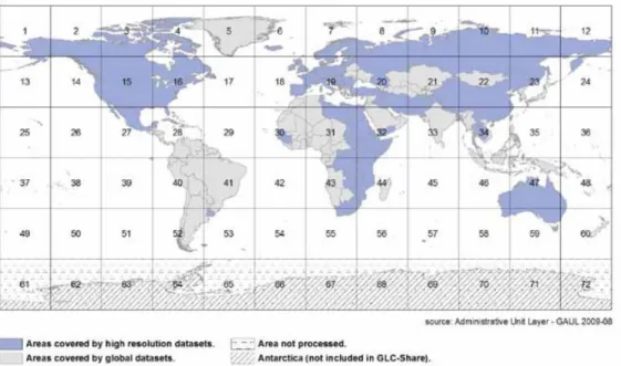
The Global Land Cover Share (GLC-Share) is produced by FAO with a resolution of 1km in
order to provide reliable land cover information for global needs. It is produced by combining
many global, regional and national datasets with the goal of “best available” global dataset.
Most of the dataset are produced by using regional or national datasets. If there is no any
regional or national datasets in a certain region they extracted the land cover from global
datasets such as; GlobCover2009, MODIS VCF-2010 and Cropland database 2012 (Latham et
al., 2014). Study area of this thesis (Portugal) is produced by using high resolution datasets
(Figure 3, box 18).
Figure 3 : Dataset distribution of GLC-Share Product
The European part of the GLC-Share is results from the combinations of Corine Land Cover
dataset provided by European Environment Agency (EEA) and Russian Federation Dataset
provided by Joint Research Center of the EC. Both datasets are derived from Landsat 30m and
provided in 2006 (Corine Land Cover) and in 2000 (Russian Federation). The legend of the
8 definition. The validation of Global Land Cover –Share was completed by 1000 validation samples and resulted with 80.2% overall accuracy (Latham et al., 2014).
Table 1 : GLC-Share Land Cover Legend and Class Definitions 2.1.1 Globeland30 Product
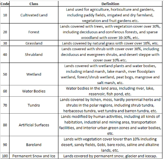
GlobeLand30 dataset is produced by National Geomatics Center of China with a resolution of
30m in 2010. They used the information derived from Landsat TM, Landsat Enhanced
Thematic Mapper Plus (ETM+) multispectral images and multispectral images of Chinese
9 and ETM+ images were collected in time period of 2009 and 2011. HJ-1 images were collected
from September 2008 to December 2011. Minimum Mapping Unit (MMU) is depending on
the class varying from 3x3 pixel to 10x10 pixel. The classification scheme of the dataset
consist of 10 classes. Table 2 shows these 10 classes and their definitions. For accuracy
assessment over 150.000 samples were used and the overall accuracy reached 83.51%. (Chen
et.al, 2015).
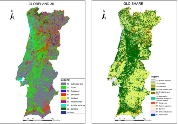
10 Table 3 presents the main characteristics of the land cover datasets used in this study.
GlobeLand30 product is produced based on the satellite images of 2010 and European part of
the GLC-Share product is based on the satellite images of 2006. Considering the temporal
differences in the products there might be some temporal changes on the land cover of the
study area. Figure 4 shows the land cover products in their original legends and colour scheme.
In study area (Continental Portugal) some of the classes doesn’t exist such as Mangroves and Snow and Glaciers classes in GLC-Share product; Tundra and Permanent Snow and Ice classes
in Globeland30 product, therefore these classes are excluded from the comparison of the
datasets.
Table 3 : Technical specification of the global land cover datasets
11
3.
EAGLE CONCEPT
Arnold et al., (2013) introduced a new concept called “EAGLE” –Environmental Information and Observation Network (EIONET) Action Group on Land Monitoring in Europe- which can
be used as a common framework for different land cover and land use maps. EAGLE concept
provides a way to compare different classification schemes and semantic translation by
decomposing classes depending on their class definitions.
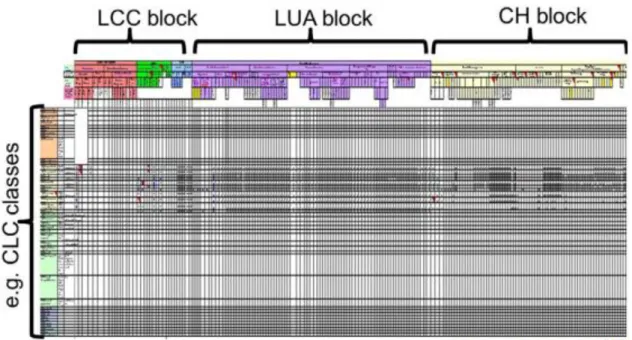
EAGLE concept consists of two different approaches to realize it’s goals; EAGLE matrix and EAGLE Unified Modeling Language (UML) model. UML model is a data model built on UML
format. EAGLE matrix is a matrix including land cover, land use and landscape characteristics
blocks where each of the blocks are consist of the decomposition of the land cover/land use
classes in a set of elements. The matrix consist of three main blocks namely, Land Cover
Components (LCC), Land Use Attributes (LUA) and Characteristics (CCH) (Figure 5).
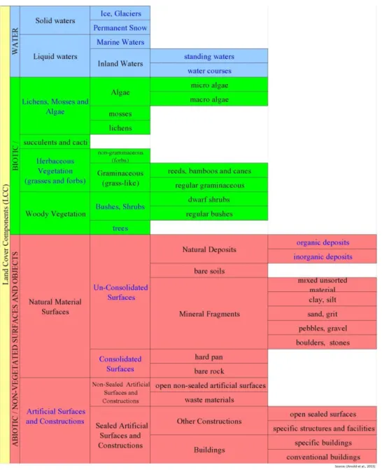
12 Each block of the matrix is hierarchically divided into subcategories in order to decompose the
classes into atomic features. In this study, we compare land cover maps based on only Land
Cover Components of the EAGLE matrix. Land Cover Components are divided into three main
categories as Abiotic/Non-vegetated, Biotic/Vegetation and Water. These subdivisions are also
divided into more detailed categories. Figure 6 shows the structure of the Land Cover
Components in the EAGLE matrix.
13
Bar Code Approach
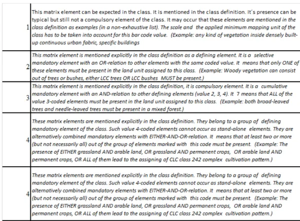
Bar code approach is a method to fill the EAGLE matrix. To apply this method each matrix
cell should be filled with a bar code number shown in Table 4. In order to define these barcode
numbers, firstly each class definition should be examined carefully in order to match with
related EAGLE Land Cover Components (LCC) attribute. One by one each EAGLE LLC
attribute should be checked and the bar codes should be filled with the codes shown in Table
4 considering the explanation of the bar code numbers.
Table 4 : Barcode method value list
Another important rule while decomposing classes is that user’s interpretation shouldn’t be included and while defining the bar code values, only the terms which are explicitly mentioned
in the class definitions should be considered. In the methodology section, a detailed example
14
4.
METHODOLOGY
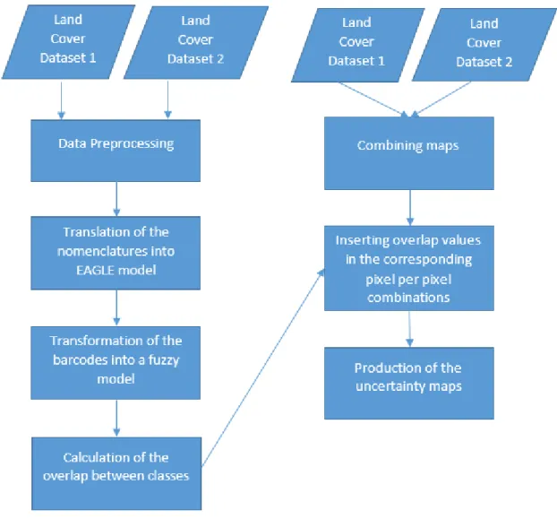
Figure 7 shows the flowchart of the methodology. The process starts with data preprocessing
of the land cover products. Afterwards, for each dataset an EAGLE matrix is created and
barcodes of the matrix are transformed into a fuzzy function. Using the fuzzy function, fuzzy
comparison approach of Ahlqvist (2005) is applied and the overlap values between classes are
calculated. Finally uncertainty maps are produced by inserting these overlap values into
combined datasets. In the next chapters the details of the methodology is explained step by
step;
15
Data Preprocessing
Firstly the global land cover data sets are cropped into official Continental Portugal borders
using the administrative borders of 2015 provided by official Portuguese institute (Direçao
Geral do Territorio). To deal with the degree of generalization, higher resolution map
resampled to lower resolution map. Globeland30 has 30m of resolution while GLC-Share
product has 1km spatial resolution. In order to have the same resolution Globeland30 product
resampled to GLC-Share product’s spatial resolution which is 1 km. Resampling is performed by using majority filter. Majority filter determines the new class of the resampled pixel based
on the most popular class, among the resampled pixels window (Webhelp.esri.com, 2015).
Translation of the Nomenclatures into EAGLE Model
Second step of methodology, which is the translation of the nomenclatures into EAGLE model,
is performed by using bar code approach which is explained in section 3. Class definitions of
the datasets are examined in depth. Definitions are decomposed using EAGLE model and each
bar code is assigned into EAGLE matrix using Table 4.
Figure 8 shows an example of bar code approach for the Grassland class in GLC-Share product.
Regarding barcode approach rules “Regular Graminaceous” attribute of EAGLE matrix is
coded 3, because it is explicitly mentioned in the class definition and it is compulsory element
of the class. Trees, regular bushes, dwarf shrubs, reeds, bamboos and canes, non graminaceous
attributes of the EAGLE matrix are coded 1, because they are mentioned in the class definition
but they are not mandatory element of the class (See Table 1 and Table 4). The rest of the
attributes coded 0 because they not mentioned in the class definition. For better visibility, in
Figure 8 EAGLE LCC attributes are divided into two parts.
Figure 9 and Figure 10 shows results of the barcode method for the land cover data sets
16
17
18
19
Calculation of the Overlap Between Classes
Ahlqvist (2005) developed an overlap metric to cope with semantic uncertainty of geographical
concepts, providing a measure of how geographical concepts are similar to each other. The
methodology provides a way to estimate the degree of overlap between classes. The overlap
degree between classes can be calculated using the following Equations:
𝜊(𝑃𝐴, 𝑃𝐵) = ∫ min(𝑓𝑃𝐴(𝑥), 𝑓𝑃𝐵(𝑥))𝑑𝑥 / ∫ 𝑓𝑃𝐵(𝑥)𝑑𝑥 (1)
In equation 1 property overlap (o) is overlap of the fuzzy functions 𝑓𝑃𝐴 and 𝑓𝑃𝐵 for properties A and B. An example of property could be the cover percentage of tree in a Forest class
definition. Minimum operator is used to define the borders of overlap between two fuzzy
functions. An example of this could be two different Forest class definitions and the borders of
overlap between two different coverage percentages.
The Overlap matric (O) evaluates how similar the concept A and concept B and it is calculated
by using Equation 2. To calculate the overlap metric between concepts A and B Equation 2 is
used where defines the importance of the property B.
Ο(𝐶𝐴, 𝐶𝐵) = √∑ 𝑊|𝑈|𝑖 𝐵𝑖∗𝜊(𝑃𝐴, 𝑃𝐵)2 (2)
In order to implement Ahlqvist’s fuzzy comparison approach in this study, barcode values from EAGLE concept transformed into a fuzzy function. Figure 11 illustrates the transformation of
values into a fuzzy function that defines the possibility of a LCC belonging to a certain land
20
Figure 11 : Transformation of the bar code values into a fuzzy function
The LCC that were assigned with the bar code values 3 and 4 have full membership to the land
cover class, because these elements are mandatory and mentioned explicitly in the class
definition. Without these elements assigned to the land unit the land cover class could not be
defined. The matrix elements with bar code value 2 are also mandatory. However the matrix
elements with bar code value 2 have an OR relation between them (see Table 4). A matrix
element with bar code value 2 could not be necessarily present in the land unit and for this
reason was assigned a membership value of 0.66. The matrix elements with bar code value 1
are not mandatory and are provided as a list of examples to define a land cover class. In this
sense the matrix elements with bar code value 1 were assigned with a membership value of
0.33. The matrix elements with bar code value 0 are not mentioned in the class description and
a membership of 0 is assigned to these elements. In this case the LCC with a bar code value 0
don't belong to a certain class and for this reason the membership value assigned to this bar
code value is 0.
4.3.1 Calculation of Land Cover Components semantic overlap;
Considering LCCA as the Land Cover Component for land cover class A, and LCCB as the Land
Cover Component for land cover class B, Equation 1 is transformed into Equation 3. The
21 defining the membership of the bar coded values of a LCC for land cover class A and land
cover class B respectively.
( , ) min( ( ), ( )) / ( )
A B B
A B LCC LCC LCC
o LCC LCC
f x f x dx f x dx (3)Due to the equation formulation of Equation 3 only the LCC that are different from 0 for land
cover class B are used in the computation of the LCC overlap, and in this sense the overlap
measure is applied in the perspective of land cover class B.
Table 5Table 1 shows an example for calculation of the LCC overlap between Forest of
GlobeLand30 and Grassland of GLC-Share products.
Table 5 : An example of calculation of LCC overlap between attributes
In Table 5, for better visibility the LCC attributes of EAGLE model which is coded ≠ 0 are
shown. 0 coded LCC attributes for Grassland (fLCCB( )x ) are discarded due the Equation 3. Using
equation 3 and Table 5 LCC overlap (o) between Forest class and Grassland class can be
calculated as below;
1. For Regular Bushes, Dwarf Shrubs, Reeds, Bamboos and Canes, Forbs and Ferns
LCC attributes ;
22 2. For Trees column,
Min (1, 0.33) / 0.33 = 1
3. For Regular Graminoids column,
Min (0.33, 1) / 1 = 0.33
Figure 6 shows another example of calculation of LCC overlaps. Using the same methodology
LCC property overlap between Cultivated Land and Tree Covered Areas are calculated.
Table 6 : Calculation of overlap of LCC for Cultivated Land class of Globeland30 product and Tree Covered Areas class of GLC-Share product
4.3.2 Determination of the weights
Considering LCCA as the Land Cover Component for land cover class A, and LCCB as the Land
Cover Component for land cover class B, Equation 2 is transformed into Equation 4.
| |
2
( , ) * ( , )
i i i
U
A B B A B
i
O C C
W o LCC LCC (4)Weights are calculated only for second land cover data set (LCCB) due to equation (4). There
is two different approaches are used to determine the weights accordingly with the information
23
1)If there is no information about land cover coverage in the description of classes;
In this case the definition of weights is based on the membership values assigned to class LCCB.
The determination of these weights are subjective and context depended because it is necessary
to assign weights to the LCCs accordingly with their importance in the definition of a land
cover class.
• The attribute with the highest membership value will have a weight of 0.9. If there is more than one same highest membership value, weight is computed by dividing 0.9 by the
remaining attributes that were assigned with same membership value.
• The attribute with the lowest membership value will have a weight of 0.1. If there is more than one same lowest membership value, weight is computed by dividing 0.1 by the
remaining attributes that were assigned with same membership value.
• If all the attributes have the same membership value the weight is set to 1. If there is more than one same membership value, weight is computed by dividing 1 by the remaining
attributes that were assigned with same membership value.
For example; in the description of Artificial Surfaces class of GLC-Share product, there is no
coverage information. Table 7 shows the LCC attributes ≠ 0 of Artificial Surfaces class of GLC-Share product and weights of the LCC attributes. The highest membership value (In this
case 0.66) will have weight of 0.9; but the highest membership value is shared by four LCC
attributes. In this case all the LCC attributes which has a membership value of 0.66, are
weighted with 0.225 (0.9 / 4 = 0.225). The rest of the membership values are consist of 0.33
and therefore 6 LCC attributes which has 0.33 membership value, are weighted with 0,017.
(0.1 / 6 = 0.017) (See Table 7).
24
2) If there is information about land cover coverage in the description of the land cover
classes;
The determination of weights are based on the land cover coverage description for class B. If
any component of LCC attribute is defined with a coverage percentage; this attribute will have
a weight of the same value as possiblity of belonging to this class. The remaining attributes
will share the remaing weights.
An example could be Grassland class in GLC-Share product. Grassland coverage is defined as
more than 10% (See Table 1). Therefore the coverage possibility of Grassland to be belonging
in this class is 90% . Table 8 shows the weights for Grassland class in GLC-Share product. The
“Regular Graminaceous” attribute has a possibility of 90% to be belonging into Grassland class, therefore will have the weight of 0.9. The remaining 0.1 is divided by the remaining LCC
attributes where the membership value is different from 0. The weights of these attributes are
defined with a value of 0.2 (The remaining weight of 0.1 is divided by remaining 5 attributes).
Table 8 : Weights for Grassland class of GLC-Share product
Another example could be the Tree Covered areas class of GLC-Share product. This class is
defined as more than 10% of tree coverage (See Table 1). Therefore the possibility of trees
attribute belonging in this class is 90% and trees attribute of LCC will have a weight of 0.9.
25
Table 9 : Weights for Tree Covered Areas Class of GLC-Share Product
4.3.3 Computation of the overlap between land cover classes
Using Equation 4 overlap between land cover classes are calculated. For example using
Equation 4 and Table 10 we can calculate overlap value between Forest class of Globeland30
and Grassland class of GLC-Share. Applying Equation 4 results with a overlap value of 45%
between Forest and Grassland classes. Figure 13 shows the overlap matrix calculated using this
methadology, for the classes of Globeland30 and GLC-Share datasets.
Table 10 : Weights and LCC Overlap Values of Forest and Grassland Classes
Production of the Uncertainty Maps
In order to produce the uncertainty maps, first step is to combine the land cover datasets. Result
of combining two land cover datasets is a map which consist of pixels where each pixel has a
value that has the class information of the corresponding pixels in each dataset. Finally,
uncertainty map is produced by inserting the overlap values into the corresponding pixels with
26
Figure 12 : Production of overlap maps process
Figure 12 illustrates the process of production of the uncertainty maps. In the example the
corresponding certain area of Globeland30 and GLC-Share products are illustrated as 4x4
pixels. Each pixel has the information of the class with a class number. Combine process
creates new 4x4 pixel area that in each pixel there is information about the classes of two land
cover maps. After combining the maps each new code is replaces with the overlap degree of
27
5.
RESULTS AND DISCUSSION
Overlap Matrix
Figure 13 shows the overlap matrix between the datasets Globeland30 and GLC-Share. The
overlap degree distribution was classified in 5 classes of overlap degree that are showed in
Table 11.
Figure 13 : Overlap matrix between GlobeLand30 legend and GLC-SHARE legend.
Overlap Overlap class [0% - 20%] Very low overlap ]20% - 40%] Low overlap ]40% - 60%] Intermediate overlap ]60% - 80%] High overlap ]80% - 100%] Very high overlap
Table 11 : Overlap classes defined for the representation of the semantic overlap.
Total overlap (1.00) occurs when the definitions of classes and decomposed EAGLE barcodes
has complete overlap. Forest-Tree Covered Areas, Grassland-Grassland, Shrubland-Shrub
28 have overlap degree of 100%. Wetland and Water Bodies, Cultivated Land and Cropland,
Cultivated Land and Tree Covered Areas, Cultivated Land and Grassland, Forest and Cropland,
Shrubland and Cropland classes have very high overlap degrees. Bareland class from
Globeland30 dataset overlaps 100% with Bare Soil and 97% with Sparse Vegetation. We can
conclude that due to close definitions of Bare Soil and Sparse Vegetation classes in GLC-Share
product, overlap between these classes are higher. Water Bodies class in both products has the
least overlap with other classes. This means that it is easier to distinguish these classes from
others semantically and these have least uncertainty degrees among the classes.
Forest class of GlobeLand30 presents an intermediate overlap degree with Cropland from
GLC-SHARE (0.61), a high value when compared with the obtained with Grassland and
Shrubs covered areas from GLC-SHARE (0,45 with both land cover classes). Indeed this value
at a first sight could be too high. However it must be presented that the overlap values were
computed just with the LCC of the EAGLE matrix, and in terms of land cover, Cultivated land
from GlobeLand30 could contain the LCCs "Trees" (e.g. olive trees or fruit trees), "Regular
bushes" (e.g. fruit berrys) and "Regular graminoids" (e.g. rainfed crops), while for Grassland
and Shrubs covered areas from GLC-Share just one of these LCCs are mandatory. This aspect
is also evident when the overlap value for Grassland and Shrubland from GlobeLand30 is
compared with Cropland from GLC-Share. If the proposed approach was extended to the Land
Use Components of the EAGLE matrix, this would result in more different features between
Cropland and the natural vegetation land cover classes of GLC-Share and consequently lower
values of semantic overlap between these land cover classes.
A similar conclusion could be withdrawal when is analyzed the Artificial surfaces from
Globeland30 overlap with Cropland, Grassland, Tree covered areas and Shrubs covered areas
from GLC-Share (an overlap value of 0,46 for Cropland and 0,42 for the remaining land cover
classes). Indeed the Artificial surfaces class description admits the presence of green urban
29
Aera Comparison
Table 12 shows the tabulated areas between Globeland30 and GLC-Share products in square
km. Table 13 shows the tabulated areas, weighted by the overlap matrix. (Figure 13). In Table
13 the class specific agreement column (ai) is calculated by summing the weighted areas by
row and dividing them by the total overlap area for the correspondent land cover class.
Table 12 : Spatial overlap areas between GLC-Share and GlobeLand30 in square Km
Table 13 shows the percentage of the conceptual semantic agreement areas between
GLC-Share and Globeland30 products throughout the study area. The table is calculated by dividing
each land cover class’ area to sum area of the column. Results shows that Forest class in Globeland30 and Tree covered Areas class in GLC-Share product has the highest spatial
overlap value with the percentage of 85. Cultivated Land and Cropland; Shrubland and Tree
Covered Areas; Wetland and Herbaceous Vegetation, Aquatic or Regularly Flooded; Grassland
and Grassland classes have relatively high spatial overlap values which is 76%, 60%, 60% and
56% respectively (See Table 13).
Conceptual overall agreement between Globeland30 and GLC-Share products throughout the
continental Portugal is %77, which is relatively high value. Forest class has the highest overlap
percentage in the dataset (%93). Cultivated Land, Grassland, Shrubland, Artificial Surfaces,
30 the dataset (%42). Although Water Bodies class is easy to distinguish from other classes the
reason of having low overlap value could be the different resolutions of the map. When
inspected the low overlap areas it can be seen that it occurs mostly in the transition zones with
water bodies and other classes. While Globeland30 product classified these zones as water
bodies due to its high resolution; GLC-Share product classified as different due to its low
resolution. GLC-SHARE 0 1 Ar tific ial su rf ac es 0 2 C ro p lan d 03 Gr ass lan d 0 4 T ree c o v er ed ar ea s 0 5 Sh ru b s co v er ed ar ea s 0 6 Aq u atic v eg etatio n , aq u atic o r reg u lar ly f lo o d ed 0 8 Sp ar se v eg etatio n 0 9 B ar e so il 1 1 W ater b o d
ies Total ai
Glo b eL an d 30
10 Cultivated land 144 27617 394 5484 311 11 22 1 0 33983 77% 20 Forest 46 1601 37 18561 141 0 28 1 0 20417 93% 30 Grassland 7 138 1083 172 45 12 6 2 0 1465 76% 40 Shrubland 29 1101 83 3706 3277 0 78 3 0 8277 60%
50 Wetland 1 3 0 2 0 56 0 0 14 76 82%
60 Water bodies 0 0 0 0 0 5 0 0 443 448 42%
80 Artificial
surfaces 1535 710 10 330 17 0 1 0 0 2603 65% 90 Bareland 3 38 21 116 39 1 595 204 0 1016 76% Total 1765 31208 1628 28370 3830 85 730 212 457 68285 a =
77%
Table 13 : Agreement areas between GlobeLand30 and GLC-SHARE in Km2 computed through the overlap matrix (Table 10). Overall agreement (a) and class specific agreement (ai) between GlobeLand30
31
Overlap Map
Overlap map is produced by inserting overlap values in each pixel and resulted with a map
showing the degree of overlap (Figure 14). Legend of the map is presented with five overlap
classes with a changing color scale from red to green. Red color represents very low overlap,
orange color represents very low overlap, yellow color represents intermediate overlap, light
green color represents high overlap and dark green color represents very high overlap values.
Although the degree of overlap across the country is relatively high, there are some hotspots
with low degree of overlap.
32
Figure 15: Very low overlap areas (A), some of the hotspots of very low overlap areas shown with satellite images (B,C)
Figure 15 (A) highlights the hotspots of very low degree of overlap (0-0.20%). In the Figure
15 (B and C), regions are overlaid with a satellite imagery provided from Esri Arcgis Word
Imagery product of the year 2013. Figure 15 (B) is located on the south-west of Portugal and
the inside the yellow box, the area is classified as Water Bodies by Globeland30 product, and
classified as Cropland by GLC-Share product. As mentioned before this area is in the transition
zone of land/water.
Figure 15 (C) shows an area with very low overlap degree. The area is classified by
Globeland30 product as Forest, GLC-Share product classified the region as Sparse Vegetation.
These classes has a degree of overlap of 16%. Checking the satellite images in the dates of
production for both of the land cover data sets (2006 and 2010), there is no significant class
change in these areas. Considering there is no temporal class change and the low degree of
33 classification error. These hotspots would help the producers to improve their datasets by
researching the reason of error. Also for the users it gives a good overview about the study
area’s agreement/disagreement.
6.
CONCLUSIONS
This dissertation provided a methodology to cope with semantic uncertainty by allowing a
fuzzy map comparison between land cover products using EAGLE Matrix Land Cover
Components. The result has been represented the semantic uncertainty spatially. Considering
case study results, the overlap degree between Globeland30 and GLC-Share products can be
considered as good in general. Provided methodology can be applied for any dataset or study
areas as well.
EAGLE matrix has been used as a semantic comparison tool which is a strong tool for semantic
comparison due to its decomposing feature. However, in this study only LCC part of the matrix
has been used and this aspect is reflected in the overlap matrix results.
Using Ahlqvist (2005) method through EAGLE LCC components highlighted the uncertainties
between classes and products by answering the question; in what degree these classes are
overlapping and where it is located? Answering these questions may advise the map makers
where to pay more attention when producing land cover maps in the future and information
about which classes are more prone to misclassification (Ran et al., 2010). Furthermore, it
would be used to highlight uncertainties for the specific classes/areas for specific applications
by the users (Fritz and See, 2008). Future work would be to include land use attributes and
characteristic blocks of the EAGLE model in order to provide more detailed comparison
34
7.
REFERENCES
Ahlqvist, O. (2005). Using uncertain conceptual spaces to translate between land cover categories. International journal of geographical information science, 19(7), 831-857.
Ahlqvist, O. (2004). A parameterized representation of uncertain conceptual spaces.
Transactions in GIS, 8(4), 493-514.
Arnold, S., Kosztra, B., Banko, G., Milenov, P., Smith, G. and Hazeu, G. (2015). EAGLE
Matrix Bar Coding Manual.
Arnold, S., Kosztra, B., Banko, G., Smith, G., Hazeu, G., Bock, M., & Valcarcel Sanz, N. (2013, June). The EAGLE concept–a vision of a future European Land Monitoring
Framework. In Proceedings of the 33rd EARSeL Symposium “Towards Horizon (Vol. 2020).
Bai, Y., Feng, M., Jiang, H., Wang, J., Zhu, Y., & Liu, Y. (2014). Assessing Consistency of Five Global Land Cover Data Sets in China. Remote Sensing, 6(9), 8739-8759.
Cabral, A., Vasconcelos, M., & Oom, D. (2010). Comparing information derived from global
land cover datasets with Landsat imagery for the Huambo Province and Guinea-Bissau. Na.
Caetano, M., and A. Araújo, 2006. Comparing land cover products CLC2000 and MOD12Q1 for Portugal. Global Developments in Environmental Earth Observation from Space (A.
Marçal, editors),Millpress, Rotterdam, pp. 469-477.
Chen, J., Chen, J., Liao, A., Cao, X., Chen, L., Chen, X., ... & Zhang, W. (2015). Global land cover mapping at 30m resolution: A POK-based operational approach. ISPRS Journal of
Photogrammetry and Remote Sensing, 103, 7-27.
Cheng, T., Molenaar, M., & Lin, H. (2001). Formalizing fuzzy objects from uncertain classification results. International Journal of Geographical Information Science, 15(1), 27-42
Comber, A., Fisher, P., & Wadsworth, R. (2004). Integrating land-cover data with different ontologies: identifying change from inconsistency. International Journal of Geographical
Information Science, 18(7), 691-708.
Comber, A., Lear, A., & Wadsworth, R. (2010). A comparison of different semantic methods for integrating thematic geographical information: the example of land cover. In 13th AGILE
International Conference on Geographic Information Science.
35 Dungan, J. L. (2006). Focusing on feature-based differences in map comparison. Journal of
Geographical Systems, 8(2), 131-143.
Fritz, S., & See, L. (2005). Comparison of land cover maps using fuzzy agreement.
International Journal of Geographical Information Science, 19(7), 787-807.
Fritz, S., & See, L. (2008). Identifying and quantifying uncertainty and spatial disagreement in the comparison of Global Land Cover for different applications. Global Change Biology, 14(5), 1057-1075.
Hagen, A. (2003). Fuzzy set approach to assessing similarity of categorical maps.
International Journal of Geographical Information Science, 17(3), 235-249.
Herold, M., Mayaux, P., Woodcock, C. E., Baccini, A., & Schmullius, C. (2008). Some challenges in global land cover mapping: An assessment of agreement and accuracy in existing 1 km datasets. Remote Sensing of Environment, 112(5), 2538-2556.
Ine.pt,. (2016). Retrieved 29 January 2016, from
https://www.ine.pt/scripts/flex_definitivos/Main.html
Kuenzer, C., Leinenkugel, P., Vollmuth, M., & Dech, S. (2014). Comparing global land-cover products–implications for geoscience applications: an investigation for the trans-boundary Mekong Basin. International Journal of Remote Sensing, 35(8), 2752-2779.
Latham, J., Cumani, R., Rosati, I., & Bloise, M. Global Land Cover SHARE (GLC-SHARE) database Beta-Release Version 1.0-2014.
National Geomatics Center of China, (2014). GlobeLand30 Product Description.
Pérez-Hoyos, A., García-Haro, F. J., & San-Miguel-Ayanz, J. (2012). Conventional and fuzzy comparisons of large scale land cover products: Application to CORINE, GLC2000, MODIS and GlobCover in Europe. ISPRS Journal of Photogrammetry and Remote Sensing, 74, 185-201.
Ran, Y., Li, X., & Lu, L. (2010). Evaluation of four remote sensing based land cover products over China. International Journal of Remote Sensing, 31(2), 391-401.
Verburg, Peter H., Kathleen Neumann, and Linda Nol. "Challenges in using land use and land cover data for global change studies." Global Change Biology 17.2 (2011): 974-989.
Weatheronline.co.uk,. (2016). Climate of the World: Portugal - Weather UK -
weatheronline.co.uk. Retrieved 29 January 2016, from
http://www.weatheronline.co.uk/reports/climate/Portugal.htm
36 http://webhelp.esri.com/arcgisdesktop/9.2/index.cfm?TopicName=resample_%28data_manag ement%29
Wu, W., Shibasaki, R., Yang, P., Ongaro, L., Zhou, Q., & Tang, H. (2008). Validation and comparison of 1 km global land cover products in China. International Journal of Remote
37